Mathematical Modelling of Glioblastomas Invasion within the Brain: A 3D Multi-Scale Moving-Boundary Approach

Abstract

Brain-related experiments are limited by nature, and so biological insights are often limited or absent. This is particularly problematic in the context of brain cancers, which have very poor survival rates. To generate and test new biological hypotheses, researchers have started using mathematical models that can simulate tumour evolution. However, most of these models focus on single-scale 2D cell dynamics, and cannot capture the complex multi-scale tumour invasion patterns in 3D brains. A particular role in these invasion patterns is likely played by the distribution of micro-fibres. To investigate the explicit role of brain micro-fibres in 3D invading tumours, in this study, we extended a previously introduced 2D multi-scale moving-boundary framework to take into account 3D multi-scale tumour dynamics. T1 weighted and DTI scans are used as initial conditions for our model, and to parametrise the diffusion tensor. Numerical results show that including an anisotropic diffusion term may lead in some cases (for specific micro-fibre distributions) to significant changes in tumour morphology, while in other cases, it has no effect. This may be caused by the underlying brain structure and its microscopic fibre representation, which seems to influence cancer-invasion patterns through the underlying cell-adhesion process that overshadows the diffusion process.

1. Introduction

Glioblastoma multiforme is a highly invasive and aggressive type of brain tumour, typically with poor patient prognosis [1,2,3,4,5,6,7] (with a median survival rate of less than one year [8]). These tumours arise from abnormal glial cells located in the central nervous system, and shortly after their appearance, they invade the surrounding tissues in a heterogeneous fashion. This heterogeneous invasion pattern leads to tumours whose outer edges are difficult or impossible to determine with current imaging technologies, including for instance magnetic resonance imaging (MRI) and diffusion tensor imaging (DTI), both of which measure the diffusion of water molecules and enable the study of brain structures.

Due to the limited experimental approaches that one can use to study the brain, researchers have started using mathematical models to provide certain biological insights that otherwise would be difficult to obtain experimentally. Such models can help predict how tumours grow for specific patients, aiding clinicians in decision-making, or they can help test and provide new hypotheses about potential anti-tumour treatments. The mathematical modelling of tumours has seen significant advances in recent decades, which have broadened our understanding of tumour dynamics and how cells interact with their environment [9,10,11,12,13,14,15,16,17,18,19,20,21,22,23,24,25,26,27,28,29,30,31,32,33]. Although the majority of these models do not restrict themselves to a specific tumour type and rather focus on general tumours, there are some models that focus on the evolution of gliomas within the brain [34,35,36,37,38,39,40,41,42]. Recently, models have also started to incorporate the structure of the brain, by including MRI and DTI scans [35,36,37,43,44,45,46]. Even though these images are generated in 3D, most of these models are simulating tumour growth in 2D and only a few of them are 3D models [43,47,48]. Moreover, the majority of published models have focused on tumour progression only on one spatio-temporal scale. However, tumour progression is characterised by various biological processes occurring on different scales, and thus their effects on the overall tumour dynamics cannot be neglected. Hence, recent efforts have been made to establish new multi-scale frameworks for tumour progression [26,27,28,29,30,35,36,37,49], which were able to capture some of these underlying multi-scale biological processes usually involving the extracellular matrix (ECM).

In this paper, we extended the general 2D multi-scale moving-boundary modelling framework introduced in [20,26] to capture the invasion of glioblastomas within a 3D fibrous brain environment. To this end, we incorporated the information provided by both the T1 weighted and DTI scans into our multi-scale framework and used the resulting model to numerically simulate the growth of 3D gliomas within the brain. We focused on a few cases showing tumour growth in different regions in the brain, with different distributions of grey/white matter densities, which leads to different tumour invasion patterns.

The model presented in this paper is a first to advance the multi-scale moving boundary modelling of 3D brain gliomas in two key ways compared to previous ones, as can be seen for instance in [35,36,37]. On the one hand, using this modelling framework, we explicitly address the micro-fibres and their rearrangement dynamics caused by the macro-scale movement of the cancer cell population (a process of great importance as the micro-scale structural changes of the underlying tissue can significantly influence the cell population motility). On the other hand, we also model another vital proteolytic process that occurs along the invasive edge of the tumour, allowing us to explicitly model tumour morphological changes and how the tumour boundary progresses over a time interval.

This paper is organised as follows. First, we formulate our extended multi-scale moving boundary framework in Section 2. Then, following a brief description of the numerical methods, we present the computational simulation results in Section 3. Finally, in Section 4, we summarise and discuss these results.

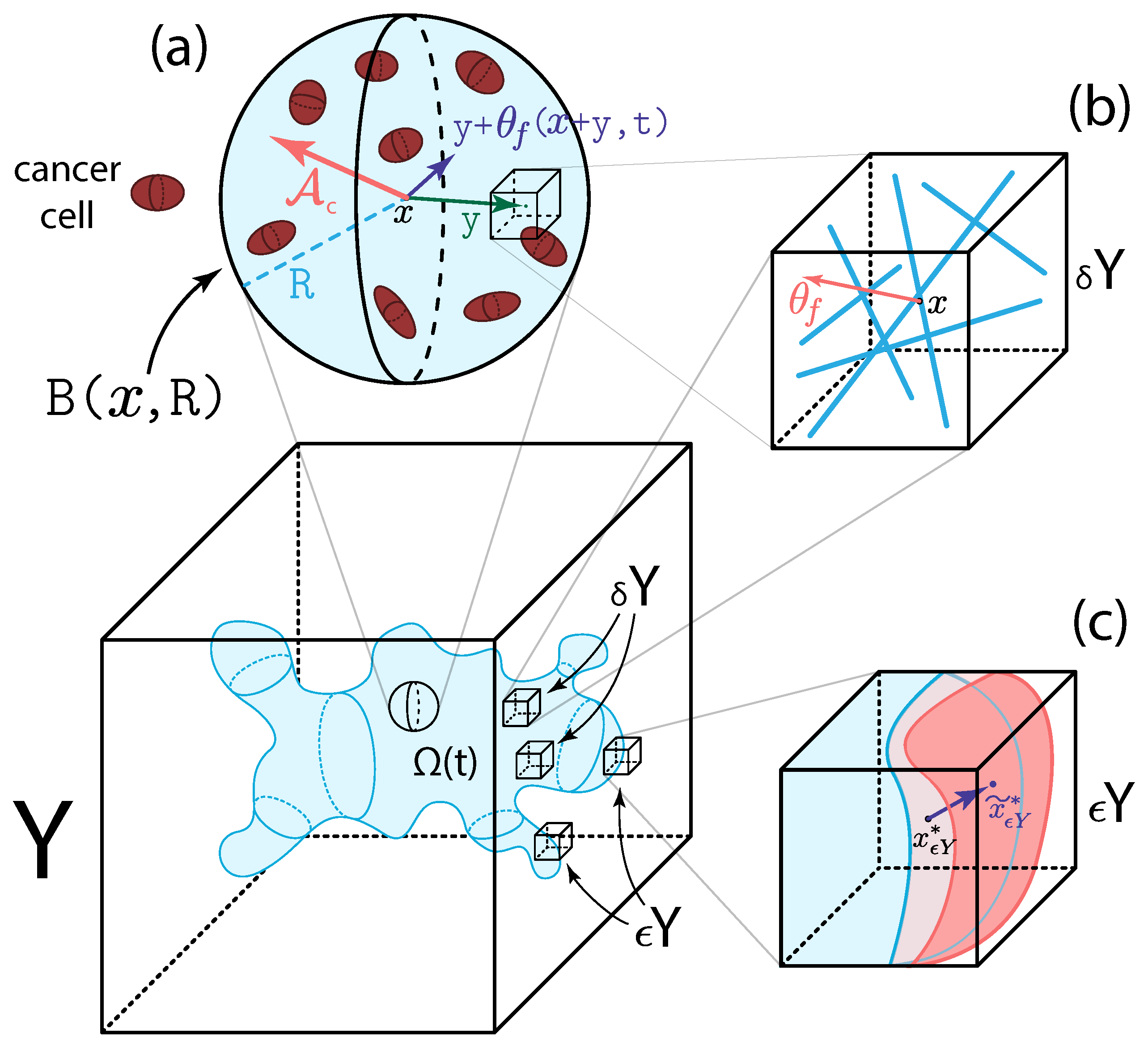
2. Multi-Scale Modelling of the Tumour Dynamics

To model the evolution of glioblastomas within a three-dimensional brain, we employ a multi-scale moving boundary model that was initially introduced in [20] and later expanded in several other works [26,27,28,29,30,49]. To account for the brain’s structure, we aim to use 3D T1 weighted and DTI scans that ultimately influence the migration of the cancer cells as well as affect both micro-scale dynamics. Hence, here we aim to explore the impact of the brain structure on the interlinked macro-scale and micro-scale tumour dynamics.

2.1. Macro-Scale Dynamics

Since in this work we extend the 2-dimensional (2D) modelling framework introduced in [20,26], we begin by briefly describing some of the key features of this framework and by giving a few useful notations. First, we denote by $\Omega \left(t\right)$ the expanding 3-dimensional (3D) tumour region that progresses over the time interval $[0,T]$ within a maximal tissue cube $Y\subset {\mathbb{R}}^N$ with $N=3$, i.e., $\Omega \left(t\right)\subset Y, \forall t\in [0,T]$; as can also be seen in Figure 1.

Then, at any macro-scale spatio-temporal point $(x,t)\in Y\times [0,T]$, we consider a cancer cell population $c(x,t)$ that is placed within and interacts with a two-phase ECM: the non-fibre $l(x,t)$ and fibre $F(x,t)$ ECM phases [26,27,28,29,30]. On the one hand, the fibre ECM phase accounts for all major fibrous proteins such as collagen and fibronectin, whose micro-scale distribution induces the spatial orientation of ECM fibres. Hence, the macro-scale spatio-temporal distribution of the ECM fibres is represented by an oriented vector field ${\theta }_f(x,t)$ that describes their spatial bias, as well as by $F(x,t):=\Vert {\theta }_f(x,t)\Vert$, which denotes the amount of fibres at a macro-scale point $(x,t)$ [26,27,28,29,30]. On the other hand, in the non-fibre ECM phase, we bundle together every other ECM constituent such as non-fibrous proteins (for example amyloid fibrils), enzymes, polysaccharides and extracellular $C{a}^{2+}$ ions [26,27,28,29,30]. Furthermore, in this new modelling study, we incorporate the structure of the brain by extracting data from DTI and T1 weighted brain scans, and then use these data to parametrise the model. Specifically, we denote by ${\mathbb{D}}_{Water}\left(x\right)$ the water diffusion tensor that is induced by the DTI scan. Furthermore, we denote by $w\left(x\right)$ the white matter density and by $g\left(x\right)$ the grey matter density, both of which are extracted from the T1 weighted image. Finally, to facilitate the description of the model and to make the mathematical notations more compact, we denote by $\mathbf{u}$ the global tumour vector which at each $(x,t)$ is given by

$$\mathbf{u}:={(c(x,t),l(x,t),F(x,t))}^{⊺}.$$

With this notation, the total space occupied by the macroscopic tissue is denoted by $\rho \left(\mathbf{u}\right)$ and is defined as

$$\rho \left(\mathbf{u}\right)=\rho \left(c\right(x,t),l(x,t),F(x,t\left)\right):=c(x,t)+l(x,t)+F(x,t).$$

2.1.1. Cancer Cell Population Dynamics

To describe the spatio-temporal evolution of the cancer cell population $c(x,t)$, we first assume a logistic-type growth with rate $\mu$ [26,27,28,29,30,50,51,52]. For the movement of this cell population, we use the structure of the brain by taking into account both the T1 weighted and DTI scans (from the IXI Dataset [53]), as well as the various adhesion-mediated processes [54,55,56,57,58,59]. Hence, the spatio-temporal dynamics of the cancer cell population is described by

$${\displaystyle \frac{\partial c}{\partial t}}=\underset{\begin{array}{c}\mathrm{fully} \mathrm{anisotropic}\\ \mathrm{diffusion}\end{array}}{\underbrace{\nabla \nabla :\left[{\mathbb{D}}_T\left(x\right)c\right]}}-\underset{\mathrm{adhesion} \mathrm{processes}}{\underbrace{\nabla ·\left[c{\mathcal{A}}_c(x,t,\mathbf{u},{\theta }_f)\right]}}+\underset{\begin{array}{c}\mathrm{logistic}-\mathrm{type}\\ \mathrm{proliferation}\end{array}}{\underbrace{\mu c{\left[1-\rho \left(\mathbf{u}\right)\right]}^{+}}}.$$

(1)

Here, the operator $\nabla \nabla :$ denotes the full second order derivative [35], i.e., it is defined as

$$\nabla \nabla :\left[{\mathbb{D}}_T\left(x\right)c\right]:=\sum _{i,j=1}^N{\displaystyle \frac{\partial }{\partial x_i}}{\displaystyle \frac{\partial }{\partial x_j}}\left({\mathbb{D}}_{i,j}c\right),\hspace{1em}N=3,$$

with ${\mathbb{D}}_{i,j}$ denoting the components of the tumour diffusion tensor ${\mathbb{D}}_T$. Since classical diffusion models with a constant coefficient cannot capture any directional cues, as those provided by the DTI data, in Equation (1), we use a tensor model (involving a fully anisotropic diffusion term) that is able to incorporate the anisotropic nature of the cancer cell movement. These tensor models were proposed in [60,61,62,63] and have been used to mathematically model the gliomas within the brain; see for instance [35,36,37]. The main idea of this approach is to use the measured water diffusivity in the structured, fibrous brain environment characterised by a symmetric water diffusion tensor [64]:

$${\mathbb{D}}_{Water}\left(x\right)=\left[\begin{array}{ccc}{d}_{xx}\left(x\right)& d_{xy}\left(x\right)& d_{xz}\left(x\right)\\ d_{xy}\left(x\right)& d_{yy}\left(x\right)& d_{yz}\left(x\right)\\ d_{xz}\left(x\right)& d_{yz}\left(x\right)& d_{zz}\left(x\right)\end{array}\right],$$

(2)

and appropriately construct a macroscopic diffusion tensor for the cancer cell population. Since this water tensor (2) is naturally symmetric (due to the DTI scans) [64], it can be diagonalised. Denoting its eigenvalues by ${\lambda }_1\left(x\right)\ge \cdots \ge {\lambda }_N\left(x\right)$ and the associated eigenvectors by ${\varphi }_1\left(x\right),\cdots {\varphi }_N\left(x\right)$, we follow [37,65,66] and construct the 3D tumour diffusion tensor as

$$\begin{array}{cc}\hfill {\mathbb{D}}_T\left(x\right):=D_c D_{WG}\left(x\right)[& \left(r+(1-r)\left({\displaystyle \frac{cothk\left(x\right)}{k\left(x\right)}}-{\displaystyle \frac{1}{k{\left(x\right)}^2}}\right)\right)I_3\hfill \\ & +(1-r)\left(1-{\displaystyle \frac{3cothk\left(x\right)}{k\left(x\right)}}+{\displaystyle \frac{3}{k{\left(x\right)}^2}}\right){\varphi }_1\left(x\right){\varphi }_1^{⊺}\left(x\right)].\hfill \end{array}$$

(3)

Here, $D_c>0$ is the diffusion coefficient, $r\in [0,1]$ specifies the degree of isotropic diffusion, $I_3$ denotes the $3\times 3$ identity matrix, and $k\left(x\right)$ is given by

$$k\left(x\right):={\mathcal{K}}_{FA}FA\left(x\right),$$

with ${\mathcal{K}}_{FA}\ge 0$ being a proportionality constant measuring the sensitivity of the cells to the environments’ direction, and $FA\left(x\right)$ denotes the fractional anisotropy index [67] given by

$$FA\left(x\right):=\sqrt{{\displaystyle \frac{{({\lambda }_1-{\lambda }_2)}^2+{({\lambda }_2-{\lambda }_3)}^2+{({\lambda }_1-{\lambda }_3)}^2}{2({\lambda }_1^2+{\lambda }_2^2+{\lambda }_3^2)}}}.$$

Finally, it is well known that the malignant glioma cells positioned in the white matter exercise quicker motility than those situated in the grey matter [39,68,69,70]. To account for this effect, in (3), we use a regulator term $D_{WG}(·)$ that is given by

$$D_{WG}\left(x\right)=a+(1-a)\left(\left(D_G g\left(x\right)+w\left(x\right)\right)\ast {\psi }_{\rho }\right)\left(x\right),$$

(4)

where $0\le D_G\le 1$ is the grey matter regulator coefficient, ∗ is the convolution operator [71], ${\psi }_{\rho }:=\psi \left(x\right)/{\rho }^N$ denotes the standard mollifier and $g\left(x\right)$ and $w\left(x\right)$ are the grey and white matter densities provided by the T1 weighted image (following an image segmentation process). Finally, $0\le a\le 1$ is a parameter that distinguishes between different cases (see Section 3).

In addition, the movement of the cancer cells is further biased by various adhesion-mediated process [54,55,56,57,58,59]. Due to the increasing evidence that gliomas induce a fibrous environment within the brain [72,73,74,75,76,77,78,79,80,81,82], in (1), we model the overall adhesion process using a non-local flux term that was introduced in [26] (see also [19,27,28,29,30,49,83,84] for similar terms). Specifically, we explore the adhesive interactions of the cancer cells at $x\in \Omega \left(t\right)$ with other neighbouring cancer cells, with the distribution of the non-fibre ECM phase [85,86,87,88] as well as with the oriented fibre ECM phase [89,90], all located within a sensing region $\mathbf{B}(x,R)$ of radius $R>0$. For this, we define the non-local flux term as

$$\begin{array}{cc}\hfill {\mathcal{A}}_c(x,t,\mathbf{u},{\theta }_f):=\frac{1}{R}\underset{\mathbf{B}(0,R)}{\int }\mathcal{K}\left(y\right)[& n\left(y\right)\left({\mathbf{S}}_{cc}c(x+y,t)+{\mathbf{S}}_{cl}l(x+y,t)\right)\hfill \\ & +\widehat{n}(y,{\theta }_f(x+y,t)){\mathbf{S}}_{cF}F(x+y,t)]{\left[1-\rho \left(\mathbf{u}\right)\right]}^{+} dy,\hfill \end{array}$$

(5)

where ${\mathbf{S}}_{cc}$, ${\mathbf{S}}_{cl}$, ${\mathbf{S}}_{cF}>0$ are the strengths of the cell–cell, cell–non-fibre ECM and cell–fibre ECM adhesions, respectively. While we take both ${\mathbf{S}}_{cl}$ and ${\mathbf{S}}_{cF}$ as positive constants, we consider the emergence of strong and stable cell–cell adhesion bonds to be positively correlated with the level of extracellular $C{a}^{+2}$ ions (one of the non-fibre ECM components) [91,92]. Hence, following the approach in [26,27,28,29,30], we describe the cell–cell adhesion strength by

$${\mathbf{S}}_{cc}(x,t):={\mathbf{S}}_{min}+({\mathbf{S}}_{max}-{\mathbf{S}}_{min})exp\left[1-{\displaystyle \frac{1}{1-{(1-l(x,t))}^2}}\right],$$

where ${\mathbf{S}}_{min}>0$ and ${\mathbf{S}}_{max}>0$ are the minimum and maximum levels of $C{a}^{+2}$ ions. Furthermore, in (5), we denote by $n(·)$ and $\widehat{n}(·,·)$ the unit radial vector and the unit radial vector biased by the oriented ECM fibres [26,27,28,29,30] defined by

$$\begin{array}{cc}\hfill n\left(y\right):=& \left\{\begin{array}{cc}{\displaystyle \frac{y}{{\Vert y\Vert }_2}}\hfill & \mathrm{if} y\in \mathbf{B}(0,R)\backslash \left\{0\right\},\hfill \\ 0\hfill & \mathrm{if} y=0,\hfill \end{array}\right.\hfill \\ \hfill \widehat{n}(y,{\theta }_f(x+y)):=& \left\{\begin{array}{cc}{\displaystyle \frac{y+{\theta }_f(x+y,t)}{\Vert y+{\theta }_f{(x+y,t)\Vert }_2}}\hfill & \mathrm{if} y\in \mathbf{B}(0,R)\backslash \left\{0\right\},\hfill \\ 0\hfill & \mathrm{if} y=0,\hfill \end{array}\right.\hfill \end{array}$$

respectively (for details on the fibre orientation ${\theta }_f$, see Section 2.2.1). Furthermore, to account for the gradual weakening of all adhesion bonds as we move away from the centre point x within the sensing region $\mathbf{B}(x,t)$ in (5), we use a radially symmetric kernel $\mathcal{K}(·)$ [29,30] given by

$$\mathcal{K}\left(y\right)=\psi \left(\frac{y}{R}\right),\hspace{1em}\forall y\in \mathbf{B}(0,R),$$

where $\psi (·)$ is the standard mollifier. Finally, in (5), a limiting term ${[1-\rho \left(\mathbf{u}\right)]}^{+}:=max(0,1-\rho \left(\mathbf{u}\right))$ is used to prevent the contribution of overcrowded regions to cell migration [84]. For a schematic of this adhesion process, we refer the reader to Figure 1a.

2.1.2. Two-Phase ECM Macro-Scale Dynamics

In addition to the cancer cell population, the rest of the macro-scale tumour dynamics are described by the two-phase ECM. Here, both fibre and non-fibre ECM phases are assumed to be simply described by a degradation term due to the cancer cell population. Hence, per unit of time, their dynamics is governed by

$$\begin{array}{cc}\hfill {\displaystyle \frac{\partial F}{\partial t}}=& -{\beta }_{F}cF,\hfill \\ \hfill {\displaystyle \frac{\partial l}{\partial t}}=& -{\beta }_{l}cl,\hfill \end{array}$$

(6)

where ${\beta }_F>0$ and ${\beta }_l>0$ are the degradation rates of the fibre and non-fibre ECM phases, respectively.

2.1.3. The Complete Macro-Dynamics

In summary, Equation (1) for cancer cells dynamics and Equation (6) for the two-phase ECM dynamics lead to the following non-dimensional PDE system describing the evolution of a tumour at macro-scale:

$$\begin{array}{cc}\hfill {\displaystyle \frac{\partial c}{\partial t}}=& \nabla \nabla :\left[{\mathbb{D}}_T\left(x\right)c\right]-\nabla ·\left[c{\mathcal{A}}_c(x,t,\mathbf{u},{\theta }_f)\right]+\mu c\left[1-\rho \left(\mathbf{u}\right)\right],\hfill \\ \hfill {\displaystyle \frac{\partial F}{\partial t}}=& -{\beta }_{F}cF,\hfill \\ \hfill {\displaystyle \frac{\partial l}{\partial t}}=& -{\beta }_{l}cl.\hfill \end{array}$$

(7)

To complete the macro-scale model description, we consider zero-flux boundary conditions and appropriate initial conditions (for instance, the ones given in Section 3).

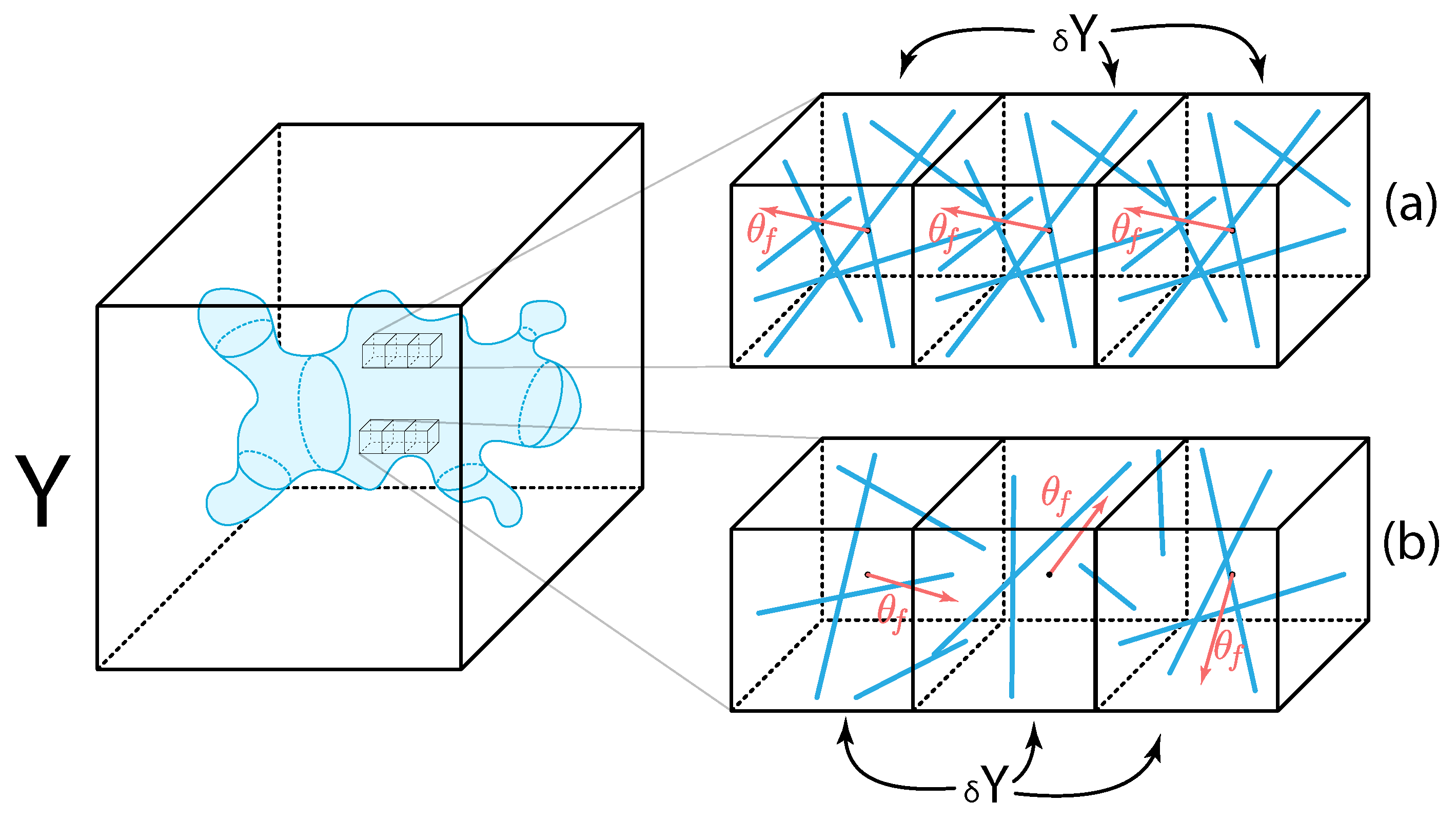
2.2. Micro-Scale Processes and the Double Feedback Loop

Since the cancer invasion process is genuinely a multi-scale phenomenon, several micro-scale processes are closely linked to the macro-scale dynamics [93]. In this work, we consider two of these micro-processes, namely the rearrangement of the ECM fibres micro-constituents [26] and the cell-scale proteolytic processes that occur at the leading edge of the tumour [20]. Here, we briefly outline these micro-processes, in addition to the naturally arising double feedback loop that ultimately connects the micro-scale and the macro-scale.

2.2.1. Two-Scale Representation and Dynamics of Fibres

To represent the oriented fibres on the macro-scale, we follow [26]. There, the authors characterised not only the amount of fibres $F(x,t)$ but also their ability to withstand incoming cell fluxes and forces through their spatial bias. By considering a cell-scale micro-domain $\delta Y\left(x\right):=x+\delta Y$ of appropriate micro-scale size $\delta >0$, both of these characteristics are induced by the microscopic fibre distribution $f(z,t)$, with $z\in \delta Y\left(x\right)$. In fact, both of these are captured though a vector field representation ${\theta }_f(x,t)$ of the ECM micro-fibres [26] that is defined as

$${\theta }_f(x,t):={\displaystyle \frac{1}{\lambda \left(\delta Y\right(x\left)\right)}}\underset{\delta Y\left(x\right)}{\int }f(z,t)dz·{\displaystyle \frac{{\theta }_{f,\delta Y\left(x\right)}(x,t)}{\Vert {\theta }_{f,\delta Y\left(x\right)}{(x,t)\Vert }_2}},$$

(8)

where $\lambda (·)$ is the Lebesgue measure in ${\mathbb{R}}^d$ and ${\theta }_{f,\delta Y\left(x\right)}(·,·)$ is the revolving barycentral orientation given by [26]

$${\theta }_{f,\delta Y\left(x\right)}(x,t):={\displaystyle \frac{\underset{\delta Y\left(x\right)}{\int }f(z,t)(z-x)dz}{\underset{\delta Y\left(x\right)}{\int }f(z,t)dz}}.$$

Hence, the fibres’ ability to withstand forces is naturally defined by this vector field representation (8) and their amount distributed at a macro-scale point $(x,t)$ is given by

$$F(x,t):=\Vert {\theta }_f{(x,t)\Vert }_2,$$

which is precisely the mean-value of the micro-fibres distributed on $\delta Y\left(x\right)$. Since both of these macro-scale oriented ECM fibre characteristics ($F(x,t)$ and ${\theta }_f(x,t)$) that we use in the macro-scale dynamics (7), genuinely emerge from the micro-scale distribution of the ECM fibres $f(z,t)$, we refer to this link as the fibres bottom-up link. An illustration of a micro-domain $\delta Y\left(x\right)$ and its corresponding macro-scale orientation ${\theta }_f(x,t)$ can be seen in Figure 1b.

On the other hand, there is also a naturally arising link that connects the macro-scale to this micro-scale, namely the fibres top-down link. This connection is initiated by the movement of the cancer cell population that triggers a rearrangement of ECM fibres micro-constituents on each micro-domain $\delta Y\left(x\right)$ (enabled by the secretion of matrix-degrading enzymes that can break down various ECM proteins). Hence, using the fact that the fully anisotropic diffusion term can be rewritten as $\nabla \nabla :\left[{\mathbb{D}}_T\left(x\right)c\right]=\nabla ·[{\mathbb{D}}_T\left(x\right)\nabla c+c\nabla ·{\mathbb{D}}_T\left(x\right)]$, the fibre rearrangement process is kicked off by the cancer cell spatial flux:

$${\mathcal{F}}_c(x,t):={\mathbb{D}}_T\left(x\right)\nabla c+c\nabla ·{\mathbb{D}}_T\left(x\right)-c{\mathcal{A}}_c(x,t,\mathbf{u},{\theta }_f),$$

(9)

which is generated by the tumour macro-dynamics (7). Then, at any spatio-temporal point $(x,t)\in \Omega \left(t\right)\times [0,T]$ this flux (9) becomes naturally balanced in a weighted fashion by the macro-scale ECM fibre orientation ${\theta }_f(·,·)$, resulting in a rearrangement flux [26]:

$$r(\delta Y\left(x\right),t):=\omega (x,t){\mathcal{F}}_c(x,t)+(1-\omega (x,t)){\theta }_f(x,t),$$

(10)

with $\omega (x,t):=c(x,t)/\left(c\right(x,t)+F(x,t\left)\right)$, that acts uniformly upon the micro-fibre distribution on each micro-domain $\delta Y\left(x\right)$. Ultimately, this macro-scale rearrangement vector (10) induces a micro-scale reallocation vector ${\nu }_{\delta Y\left(x\right)}(z,t)$ [26], enabling us to appropriately calculate the new position $z^{\ast }$ of any micro-node $z\in \delta Y\left(x\right)$ as

$$z^{\ast }:=z+{\nu }_{\delta Y\left(x\right)}(z,t).$$

(11)

For further details on the micro-fibre rearrangement process, we refer the reader to Appendix B and [26,27,28,29,30].

2.2.2. MDE Micro-Dynamics and Its Links

The second micro-scale process that we take into consideration is the proteolytic molecular process that occurs along the invasive edge of the tumour and is driven by the cancer cells’ ability to secrete several types of matrix-degrading enzymes (MDEs) (for instance, matrix-metalloproteinases) within the proliferating rim [94,95,96,97,98]. Subsequently to the secretion, these MDEs are subject to spatial transport within a cell-scale neighbourhood of the tumour interface and, as a consequence, they degrade the peritumoral ECM, resulting in changes of tumour boundary morphology [93].

To explore such a micro-scale process, we adopt the approach that was first introduced in [20] where the emerging spatio-temporal MDEs micro-dynamics is considered on an appropriate cell-scale neighbourhood of the tumour boundary $\partial \Omega \left(t\right)$. This neighbourhood is represented by a time-dependent bundle of overlapping cubic micro-domains ${\left\{ϵY\right\}}_{ϵY\in \mathcal{P}\left(t\right)}$, with $ϵ>0$ being the size of each micro-domain $ϵY$, which allows us to decompose the overall MDE micro-process, transpiring on ${\bigcup }_{ϵY\in \mathcal{P}\left(t\right)}ϵY$, into a union of proteolytic micro-dynamics occurring on each $ϵY$; see also Figure 1c. Hence, choosing an arbitrary micro-domain $ϵY$ and a macroscopic time instance $t_0\in [0,T]$, we follow the evolution of the MDE micro-dynamics during the time period $[t_0,t_0+\Delta t]$, with appropriately chosen $\Delta t>0$ and within the associated micro-domain $ϵY$. By denoting the spatio-temporal distribution of MDEs by $m(y,\tau )$ at any micro-point $(y,\tau )\in ϵY\times [0,\Delta t]$, we observe that the cancer cell population, located within an appropriately chosen distance ${\gamma }_h>0$ from $y\in ϵY$, induce a source $h(y,\tau )$ of MDEs which can be mathematically described via a non-local term [20]:

$$h(y,\tau )=\left\{\begin{array}{cc}{\displaystyle \frac{\underset{\mathbf{B}(y,{\gamma }_h)\cap \Omega \left(t_0\right)}{\int }c(x,t_0+\tau ) dy}{\lambda (\mathbf{B}(y,{\gamma }_h)\cap \Omega \left(t_0\right))}}\hfill & y\in ϵY\cap \Omega \left(t_0\right),\hfill \\ 0\hfill & y\notin ϵY\backslash (\Omega \left(t_0\right){+\{z\in Y | \parallel z\parallel }_2<\rho \left\}\right),\hfill \end{array}\right.$$

(12)

where $0<\rho <{\gamma }_h$ is a small mollification range and $\mathbf{B}(y,{\gamma }_h)$ denotes the ${\Vert ·\Vert }_{\infty }$ ball of radius ${\gamma }_h$ centred at a micro-node y. Since the calculation of this micro-scale MDE source (12) directly involves the macro-scale cancer cell population $c(·,·)$, we observe a naturally arising MDE top-down link that connects the macro-scale to the MDE micro-scale. In fact, such a source term (12) allows us to describe the spatio-temporal evolution of the MDEs’ micro-scale distribution $m(·,·)$ by [20]

$$\begin{array}{cc}\hfill {\displaystyle \frac{\partial m}{\partial \tau }}& =D_m\Delta m+h(y,\tau ),\hfill \\ \hfill m(y,0)& =0,\hfill \\ \hfill {\displaystyle \frac{\partial m}{\partial n}}{|}_{\partial ϵY}& =0,\hfill \end{array}$$

(13)

where $D_m>0$ is the constant MDEs diffusion coefficient and n denotes the outward normal vector. As it was shown in [20], we can use the solution of the MDEs micro-dynamics (13) to acquire both the movement direction and magnitude of a tumour boundary point $x_{ϵY}^{\ast }$ within the peritumoral area covered by the associated boundary micro-domain $ϵY$. This ultimately causes a boundary movement, and as a consequence, we obtain a new evolved tumour macro-domain $\Omega (t_0+\Delta t)$, the link of which we refer to as the MDE bottom-up link. For the illustration of the boundary movement, we refer the reader to Figure 1c and for further details of the MDE micro dynamics, see Appendix C or [20,26,27,28,29,30].

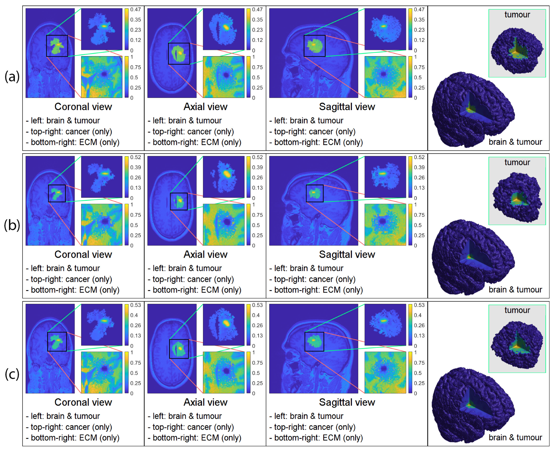
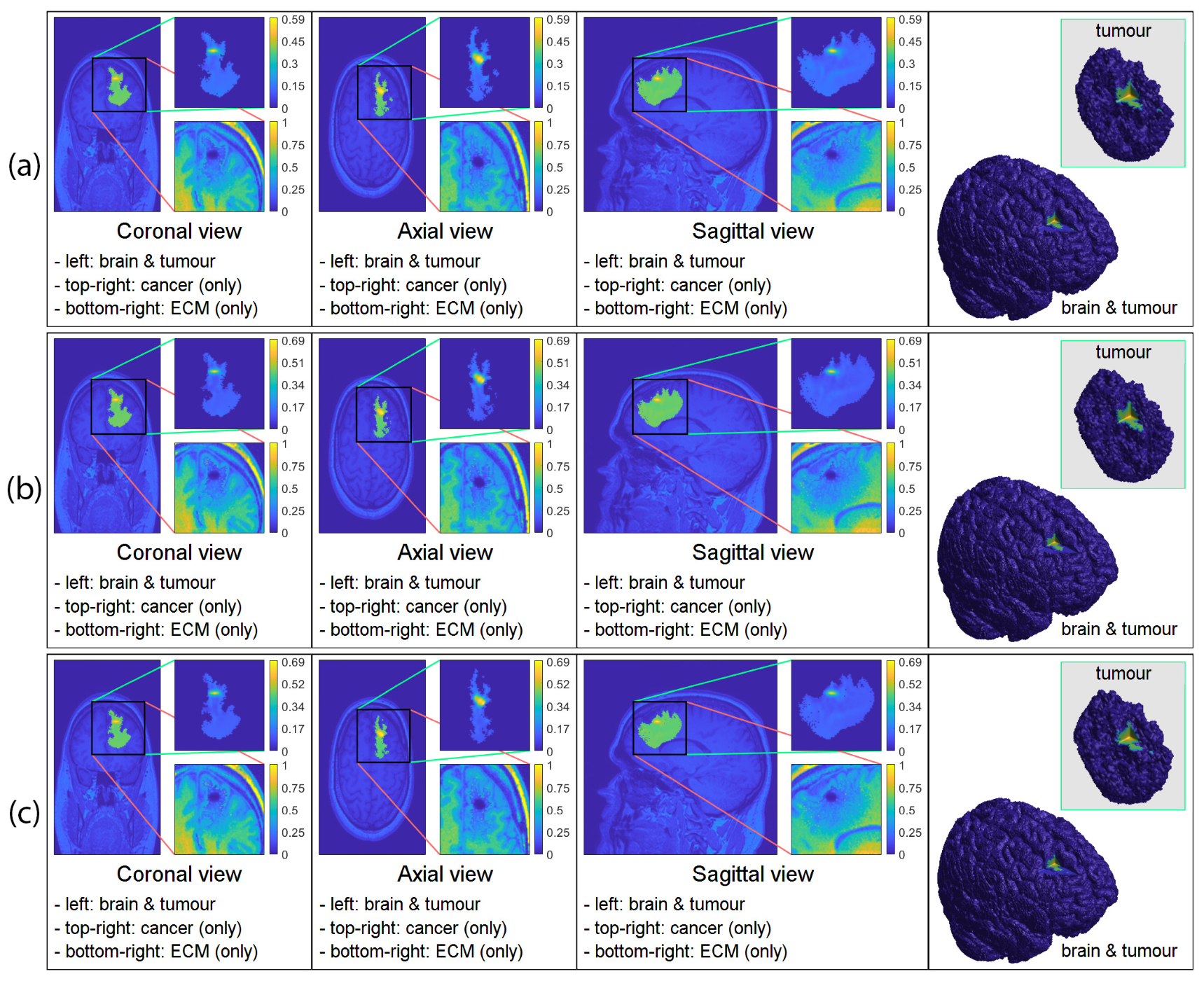
3. Computational Results: Numerical Simulations in 3D

We start this section by briefly discussing the numerical method that we use to solve the macro-scale dynamics (7), and for details on the numerical approach used for the two micro-scale dynamics (fibres and MDE), we refer the reader to [29,30]. Here, we use the method of lines’ approach to discretise the macro-scale tumour dynamics (7) first in space, and then, for the resulting system of ODEs, we employ a non-local predictor–corrector scheme [26]. In this context, we carry out the spatial discretisation on a uniform grid, where both spatial operators (fully anisotropic diffusion and adhesion) are accurately approximated in a convolution-driven fashion. First, we note that the fully anisotropic diffusion term can be split into two parts:

$$\nabla \nabla :\left[{\mathbb{D}}_T\left(x\right)c\right]=\underset{\mathrm{diffusive}}{\underbrace{\nabla ·\left[{\mathbb{D}}_T\left(x\right)\nabla c\right]}}+\underset{\mathrm{advective}}{\underbrace{\nabla ·\left[c\nabla ·{\mathbb{D}}_T\left(x\right)\right]}},$$

(14)

which enable us to use a combination of two appropriate distinct schemes for an accurate approximation. While for the diffusive part in (14), we use the symmetric finite difference scheme [99,100], for the combination of the advective (14) and adhesion operators (5) (i.e., $\nabla ·\left[c\left({\mathcal{A}}_c(x,t,\mathbf{u},{\theta }_f)+\nabla ·{\mathbb{D}}_T\left(x\right)\right)\right]$), we use the standard first-order upwind finite difference scheme which ensures positivity and helps avoiding spurious oscillations in the solution. Finally, to approximate the adhesion integral ${\mathcal{A}}_c(x,t,\mathbf{u},{\theta }_f)$, we consider an approach similar to [29,30], and use $N_s$ random points located within the sensing region $\mathbf{B}(0,R)$ and sums of discrete-convolutions.

3.1. Initial Conditions

For the numerical simulations presented in this paper, we consider the tissue cube $Y=[0,4]\times [0,4]\times [0,4]$ with the following initial condition for the cancer cells:

$$c(x,0)={\displaystyle \frac{1}{2}}exp\left({\displaystyle \frac{-{\Vert x\Vert }_2^2}{0.02}}\right)·{\chi }_{\mathbf{B}\left(\right(2,2,2),0.25)},$$

and for the non-fibre ECM phase, the initial condition $l(x,0)$ was acquired by appropriately scaling the T1 weighted image via a normalising constant. Current DTI scans do not provide suitable resolution to determine the underlying micro-fibre distributions, and so here we describe the initial micro-fibre distribution within a micro-domain $\delta Y\left(x\right)$ as follows. When the macro-scale point x that corresponds to the micro-domain $\delta Y\left(x\right)$ is located in the grey matter, then within $\delta Y\left(x\right)$, we randomly draw straight lines until the ratio between the points that belong and the points that do not belong to the collection of lines is approximately $35\%$:$65\%$. On the other hand, when the point x is located within the white matter, we use a set of predefined lines with the same point ratio ($35\%$:$65\%$), ultimately achieving a random orientation within the grey matter and an aligned orientation within the white matter [101]. Finally, the grey matter’s fibre density is assumed to be $1/D_G$ times smaller than the density in the white matter [101]. A schematics of this initial condition for the micro-fibres can be seen in Figure 2. Hence, we also incorporated the information about the white and grey matter tracks provided by the T1 weighted image into our micro-scale fibre distribution.

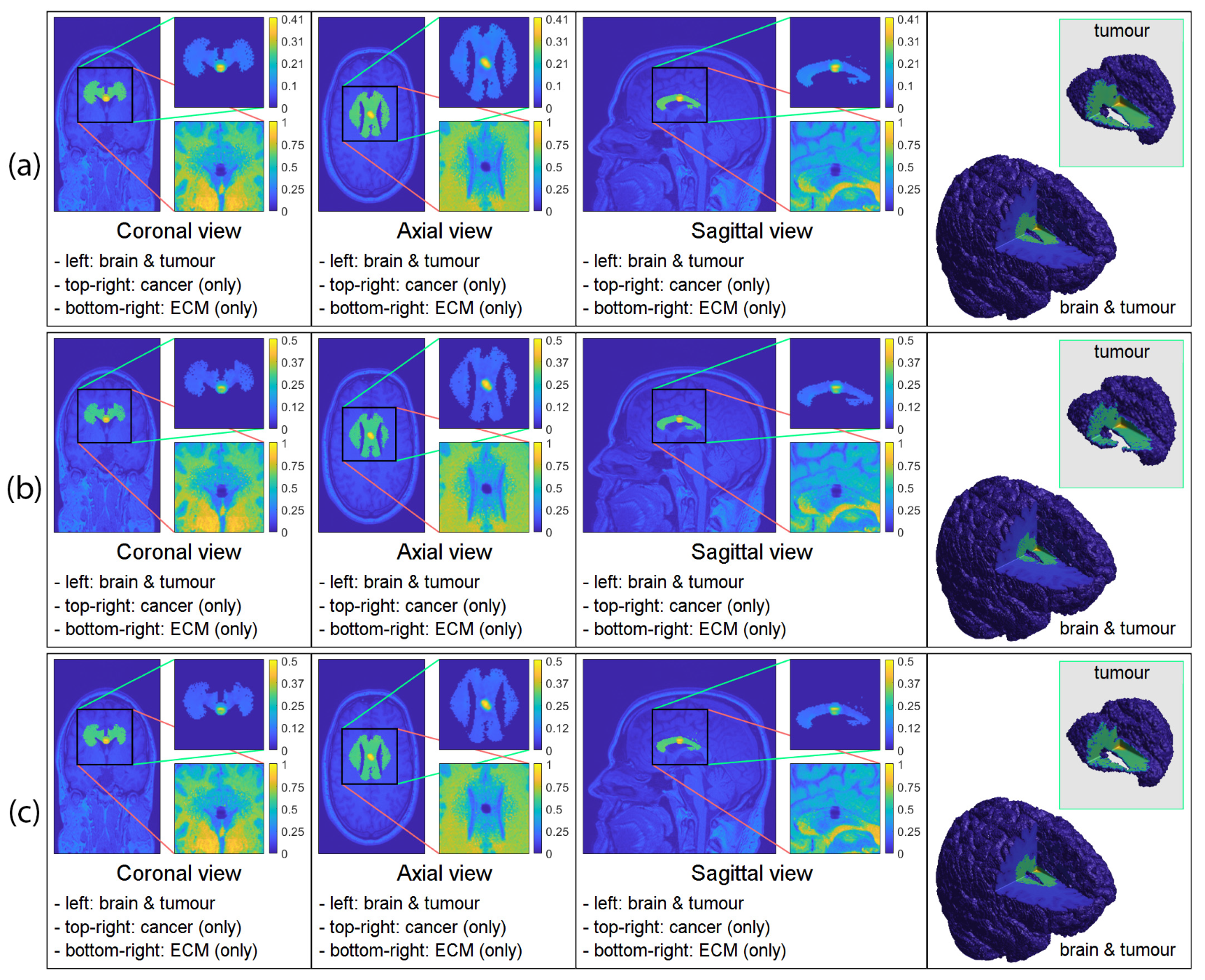
3.2. Numerical Simulations in 3D

Here, we present the 3D numerical solutions of the multi-scale model described above, for the parameter values listed in

Table A1. Parameter set used for the numerical simulations.

Variable	Value	Description	Reference
$D_c$	$1.25\times {10}^{-4}$	Diffusion coeff. for the cancer cell population	[37]
$D_G$	$0.25$	Grey matter regulator coefficient	Estimated
r	$0.1$	Degree of randomised turning	[37]
a	0	Model switching parameter	Estimated
${\mathcal{K}}_{FA}$	100	Cell’s sensitivity to the directional information	[37]
${\mathbf{S}}_{max}$	$0.5$	Cell–cell adhesion coeff.	[26]
${\mathbf{S}}_{min}$	$0.01$	Minimum level of cell–cell adhesion	[29]
${\mathbf{S}}_{cl}$	$0.01$	Cell–non-fibre adhesion coeff.	[26]
${\mathbf{S}}_{cF}$	$0.3$	Cell–fibre adhesion coeff.	[19]
$\mu$	$0.25$	Proliferation coeff. for cancer cell population	[19]
${\beta }_F$	$1.5$	Degradation coeff. of the fibre ECM	[30]
${\beta }_l$	$3.0$	Degradation coeff. of the non-fibre ECM	[30]
$\beta$	$0.8$	Optimal tissue environment controller	[20]
R	$0.15$	Sensing radius	[26]
$f_{max}$	$0.636$	Maximum of micro-fibre density at any point	[26]
$\Delta x$	$0.03125$	Macro-scale spatial step-size	[20]
$ϵ$	$0.0625$	Size of a boundary micro-domain $ϵY\left(x\right)$	[20]
$\delta$	$0.03125$	Size of a fibre micro-domain $\delta Y\left(x\right)$	[26]
$N_s$	450	Number of random points used for the	Estimated
		approximation of the adhesion integral ${\mathcal{A}}_c$

in Appendix A (any alteration from these values will be stated accordingly). To display the advanced tumours at time $50\Delta t$, we show four panels for each simulation result. In the first three panels, we show the three classical cross-section planes, i.e., the coronal plane (the head of the subject is viewed from behind), the axial plane (the head of the subject is viewed from above) and the sagittal plane (the head of the subject is viewed from the left). In the last panel of each simulation, we show the 3D image of the brain with the embedded tumour alongside the 3D tumour in isolation.

The three figures shown below investigate tumour evolution when the initial tumour starts in different regions of the brain. To present the simulations, we divide each result into four panels: coronal, axial, sagittal and 3D view. Within each coronal, axial and sagittal views, we show the tumour embedded within the brain on the left, the cancer cell density on the top-right and the ECM density on the bottom-right. In the 3D view (the furthest right panel in each result), we show the cross-section of the whole brain with the tumour in the bottom-left corner and in the top-right corner, we show the isolated tumour.

In Figure 3, we present three distinct cases obtained by varying different parameters that appear in the tumour diffusion tensor ${\mathbb{D}}_T\left(x\right)$ defined in (3). In Figure 3a, we assume that the tensor ${\mathbb{D}}_T\left(x\right)$ depends on the white–grey matter and for this purpose we set $r=1$ in (3) and $a=0$ in (4); this results in isotropic tumour diffusion. In Figure 3b, we use the DTI data (i.e., there is no a priori assumption about the preferential direction for cell movement in white matter) and thus we set $a=1$ in (4) (with $r=0.1$, as in Table A1); this results in an anisotropic diffusion that does not explicitly depend on the white–grey matter. In Figure 3c, we use both DTI data and the white–grey matter dependency (i.e., $r=0.1$ and $a=0$), with the baseline parameters from Table A1. Here, it is worth mentioning that even though we do not use the T1 weighted image to obtain the functions $w\left(x\right)$ and $g\left(x\right)$ that appear in $D_{WG}$ (such as $D_{WG}=1$ in Figure 3b, since $a=1$) we still use the T1 weighted image to initialise the micro-scale non-fibre initial density as well as the initial micro-scale fibre distributions as described above.

In all these simulations shown in Figure 3, we place the small initial tumour in the middle-right part of the brain, and we show the results of the three cases at time $50\Delta t$ where we observe significant tumour morphology changes across the three cases. By comparing Figure 3a,b and Figure 3b,c, we see that when we include the white–grey matter dependency function $D_{WG}$ within the tumour diffusion tensor, it leads to a more advanced tumour. On the other hand, comparing Figure 3a with Figure 3c shows that including the DTI data, which creates an anisotropic tumour diffusion term, leads to a slight reduction in tumour spread. Furthermore, in all three cases, we can notice that the advancing tumour tends to mostly follow the white matter tracks and usually avoids the invasion of tissues located in the grey matter. This invasion resulted in the degradation (and rearrangement) of the ECM that we can see in the bottom-right of each panel (coronal, axial and sagittal) which enabled the tumour to further expand into the surrounding tissues.

In Figure 4, we keep the same three cases as in Figure 3, i.e., Figure 4a only white-grey matter dependency, Figure 4b only DTI data and Figure 4c both. However, here we place the initial tumour in the front-right part of the brain and show the results of tumour invasion at the final time $50\Delta t$. Due to the initial position of the tumour, we can see a tumour that is growing away from the skull towards the centre of the brain as well as it is mainly following the white matter. This creates a highly heterogeneous elongated tumour with many branching outgrowths. On the other hand, in Figure 4 we only see slight differences between the three cases. This contradicts the results from Figure 3 and suggests that both the DTI data and white-grey matter dependency may not always be decisive factor in tumour morphology.

Similarly to Figure 3 and Figure 4, in Figure 5 we keep the same three cases (Figure 5a only white–grey matter dependency Figure 5b only DTI data and Figure 5c both) while we place the initial tumour mass in the middle of the brain and present the results at time $50\Delta t$. As a consequence of the initial location, we see a “butterfly”-shaped tumour that branched to both the left and right side of the brain with some asymmetry. Furthermore, as in Figure 4, we can see that all three cases are quite similar, and so the additional information provided by both the DTI data and white–grey matter dependency seems to be unnecessary for this initial condition. However, we must note that the initial conditions (fibre and non-fibre ECM) still use the information provided by the T1 weighted image, and so here, we only investigate the effect of changing the diffusion tensor.

As we mentioned, we see significant differences between the three cases only in Figure 3. This either indicates that the anisotropic diffusion tensor only provides valuable information in certain cases or that the initial micro-fibre density differs from the one that produced the DTI scan, (i.e., the actual distribution). Since we use an artificial micro-fibre structure that does not depend on the DTI scan which also aids the movement of the cancer cell population via the adhesion integral ${\mathcal{A}}_c(·,·,·,·)$ defined in (5), it is possible that in this specific case, the micro-scale fibre distribution introduced a significantly different travelling direction than the DTI data, resulting in discrepancies between the simulations. However, due to the resolution of current DTI scans, it is not possible to construct a unique fibre distribution within a micro-domain $\delta Y\left(x\right)$. Hence, to genuinely capture the underlying brain structures that we can use within a mathematical model, our results suggest that DTI scans with their present resolution may not be sufficient, and one might need to look into either obtaining better resolution DTI scans or combine this with the strength of different technologies such as magnetic resonance elastography. Nonetheless, this exceeds the current scope of this work and requires further investigation.

4. Discussion and Final Remarks

In this study, we further extended the 2D multi-scale moving-boundary framework previously introduced in [20,26], by developing it into 3D and applying it to the study of glioma invasion within the brain. Since experiments are limited within the brain, we focused on incorporating DTI and T1 weighted scans into our framework to provide insights into the structure of the brain, the tumour, and the surrounding tissue.

The original framework developed in [20,26] modelled a generic tumour in a 2D setting, and so to model gliomas within a 3D brain, we extended this modelling approach by considering the structural information provided by both DTI and T1 weighted scans. We used both DTI and T1 weighted scans to construct the tumour diffusion tensor ${\mathbb{D}}_T\left(x\right)$ defined in (3), which resulted in a fully anisotropic diffusion term. While the T1 weighted image can give different diffusion rates based on whether the cancer cells are located in the white or grey matter, the DTI data are used to incorporate the underlying brain structure and to give higher diffusion rates along specific directions based on how the measured water molecules behaved within the brain. The T1 weighted image, which provided the white–grey matter densities, were also used in our initial conditions for both ECM phases. Hence, the initial density of the non-fibre ECM phase was taken as a normalised version of the T1 weighted image, and the initial condition of the micro-fibre distribution and magnitude were also considered to be dependent on the white–grey matter structure. Furthermore, as the available DTI scans lack the adequate resolution required to construct more appropriate micro-fibre distributions, in this work, we considered a simple case where we set the fibre distributions to be either random or oriented based on whether they are positioned in the grey or white matter, respectively.

Therefore, compared to other previous 3D models such as those in [35,36,37], here we can explicitly capture the underlying tissue structure changes via the micro-fibre rearrangement process and trace how the boundary of the tumour changes over time. Moreover, the cancer cells’ movement is not only influenced by the T1 weighted and DTI scans (through an anisotropic diffusion term), but also biased by crucial non-local adhesions such as cell–cell and cell–fibre ECM adhesion, the latter of which is naturally interconnected to the tissue structural changes. Hence, our model presents a novel approach that can incorporate several vital processes for tumour development and have not been available in other previous models. This allowed us to produce exciting and valuable results/outcomes which provide further insights into the overall tumour development process.

To this end, we used this new 3D model to explore the effects of the anisotropic diffusion term for the cancer cell population. Our numerical simulations in Figure 3 show that including an anisotropic diffusion term may lead to significant changes in the overall tumour morphology. However, it seems that these changes depend on the position of the tumour inside the brain, as Figure 4 and Figure 5 do not exhibit changes consistent with the ones observed between the three sub-panels of Figure 3. This may be the result of the underlying brain structure and its microscopic fibre representation, which seems to take a leading role in influencing cancer-invasion patterns through the underlying cell-adhesion process (see Equation (5)), thus overshadowing the diffusion process. More precisely, the simplified fibre representation might not be sufficient for Figure 3, where the initial tumour was positioned in the right-middle part of the brain. However, this fibre representation might be enough for Figure 4 (with the tumour positioned in the front-right of the brain) and for Figure 5 (with the tumour positioned in the middle of the brain), where we did not see significant morphological differences between the three sub-panels considered in each of these figures.

To conclude this study, we mention that further investigation is needed to determine whether these changes in tumour invasion patterns are caused by the lack of directional information on the fibre micro-scale level or an anisotropic diffusive cell motility is necessary to better represent the invasion process. A feasible approach would also be to use a new imaging technology called magnetic resonance elastography, but this is beyond the scope of this current work. Nonetheless, these results are not only interesting and important from a mathematical modelling point of view but from a medical one as well. For instance, we showed how different model parameters change the evolution of the tumour boundary, this being a vital and desired datum in any clinical/medical decision-making process. Such a model with tuned parameters (to specific patients) could help, for example, decide the optimal amount of tissue to resect so that the chance of survival is maximised.

Finally, as our simulations are able to reproduce known tumour patterns of clinically seen growth, future experiments will be refined by prospectively collected MRI data from glioma patients and also incorporate the effects of their radiotherapy and chemotherapy treatments.

References

1. Burri, S.H.; Gondi, V.; Brown, P.D.; Mehta, M.P. The Evolving Role of Tumor Treating Fields in Managing Glioblastoma. Am. J. Clin. Oncol. 2018, 41, 191–196. [Google Scholar] [CrossRef]
2. Davis, M. Glioblastoma: Overview of Disease and Treatment. Clin. J. Oncol. Nurs. 2016, 20, S2–S8. [Google Scholar] [CrossRef] [Green Version]
3. Klopfenstein, Q.; Truntzer, C.; Vincent, J.; Ghiringhelli, F. Cell lines and immune classification of glioblastoma define patient’s prognosis. Br. J. Cancer 2019, 120, 806–814. [Google Scholar] [CrossRef] [Green Version]
4. Louis, D.N.; Ohgaki, H.; Wiestler, O.D.; Cavenee, W.K.; Burger, P.C.; Jouvet, A.; Scheithauer, B.W.; Kleihues, P. The 2007 WHO Classification of Tumours of the Central Nervous System. Acta Neuropathol. 2007, 114, 97–109. [Google Scholar] [CrossRef] [Green Version]
5. Meneceur, S.; Linge, A.; Meinhardt, M.; Hering, S.; Löck, S.; Bütof, R.; Krex, D.; Schackert, G.; Temme, A.; Baumann, M.; et al. Establishment and Characterisation of Heterotopic Patient-Derived Xenografts for Glioblastoma. Cancers 2020, 12, 871. [Google Scholar] [CrossRef] [Green Version]
6. Preusser, M.; de Ribaupierre, S.; Wöhrer, A.; Erridge, S.C.; Hegi, M.; Weller, M.; Stupp, R. Current concepts and management of glioblastoma. Ann. Neurol. 2011, 70, 9–21. [Google Scholar] [CrossRef]
7. Sottoriva, A.; Spiteri, I.; Piccirillo, S.G.M.; Touloumis, A.; Collins, V.P.; Marioni, J.C.; Curtis, C.; Watts, C.; Tavare, S. Intratumor heterogeneity in human glioblastoma reflects cancer evolutionary dynamics. Proc. Natl. Acad. Sci. USA 2013, 110, 4009–4014. [Google Scholar] [CrossRef] [Green Version]
8. Brodbelt, A.; Greenberg, D.; Winters, T.; Williams, M.; Vernon, S.; Collins, V.P. Glioblastoma in England: 2007–2011. Eur. J. Cancer 2015, 51, 533–542. [Google Scholar] [CrossRef] [PubMed] [Green Version]
9. Anderson, A.; Chaplain, M.; Newman, E.; Steele, R.; Thompson, A. Mathematical modelling of tumour invasion and metastasis. J. Theorl. Medic. 2000, 2, 129–154. [Google Scholar] [CrossRef] [Green Version]
10. Anderson, A.R.; Hassanein, M.; Branch, K.M.; Lu, J.; Lobdell, N.A.; Maier, J.; Basanta, D.; Weidow, B.; Narasanna, A.; Arteaga, C.L.; et al. Microenvironmental Independence Associated with Tumor Progression. Cancer Res. 2009, 69, 8797–8806. [Google Scholar] [CrossRef] [PubMed] [Green Version]
11. Anderson, A.R.A. A hybrid mathematical model of solid tumour invasion: The importance of cell adhesion. Math. Medic. Biol. 2005, 22, 163–186. [Google Scholar] [CrossRef] [PubMed]
12. Basanta, D.; Simon, M.; Hatzikirou, H.; Deutsch, A. Evolutionary game theory elucidates the role of glycolysis in glioma progression and invasion. Cell Prolif. 2008, 41, 980–987. [Google Scholar] [CrossRef] [PubMed]
13. Basanta, D.; Scott, J.G.; Rockne, R.; Swanson, K.R.; Anderson, A.R.A. The role of IDH1 mutated tumour cells in secondary glioblastomas: An evolutionary game theoretical view. Phys. Biol. 2011, 8, 015016. [Google Scholar] [CrossRef] [PubMed]
14. Böttger, K.; Hatzikirou, H.; Chauviere, A.; Deutsch, A. Investigation of the Migration/Proliferation Dichotomy and its Impact on Avascular Glioma Invasion. Math. Model. Nat. Phenom. 2012, 7, 105–135. [Google Scholar] [CrossRef] [Green Version]
15. Chaplain, M.; Lolas, G. Mathematical modelling of cancer cell invasion of tissue: The role of the urokinase plasminogen activation system. Math. Model. Meth. Appl. Sci. 2005, 15, 1685–1734. [Google Scholar] [CrossRef] [Green Version]
16. Chaplain, M.A.J.; Lolas, G. Mathematical modelling of cancer invasion of tissue: Dynamic heterogeneity. Netw Heterog Media 2006, 1, 399–439. [Google Scholar] [CrossRef]
17. Deakin, N.E.; Chaplain, M.A.J. Mathematical modelling of cancer cell invasion: The role of membrane-bound matrix metalloproteinases. Front. Oncol. 2013, 3, 1–9. [Google Scholar] [CrossRef] [Green Version]
18. Deisboeck, T.S.; Wang, Z.; Macklin, P.; Cristini, V. Multiscale Cancer Modeling. Annu. Rev. Biomed. Eng. 2011, 13, 127–155. [Google Scholar] [CrossRef] [Green Version]
19. Domschke, P.; Trucu, D.; Gerisch, A.; Chaplain, M. Mathematical modelling of cancer invasion: Implications of cell adhesion variability for tumour infiltrative growth patterns. J. Theor. Biol. 2014, 361, 41–60. [Google Scholar] [CrossRef] [Green Version]
20. Trucu, D.; Lin, P.; Chaplain, M.A.J.; Wang, Y. A Multiscale Moving Boundary Model Arising In Cancer Invasion. Multiscale Model. Simul. 2013, 11, 309–335. [Google Scholar] [CrossRef]
21. Hatzikirou, H.; Brusch, L.; Schaller, C.; Simon, M.; Deutsch, A. Prediction of traveling front behavior in a lattice-gas cellular automaton model for tumor invasion. Comput. Math. Appl. 2010, 59, 2326–2339. [Google Scholar] [CrossRef] [Green Version]
22. Kiran, K.L.; Jayachandran, D.; Lakshminarayanan, S. Mathematical modelling of avascular tumour growth based on diffusion of nutrients and its validation. Can. J. Chem. Eng. 2009, 87, 732–740. [Google Scholar] [CrossRef]
23. Knútsdóttir, H.; Pálsson, E.; Edelstein-Keshet, L. Mathematical model of macrophage-facilitated breast cancer cells invasion. J. Theor. Biol. 2014, 357. [Google Scholar] [CrossRef] [PubMed]
24. Macklin, P.; McDougall, S.; Anderson, A.R.A.; Chaplain, M.A.J.; Cristini, V.; Lowengrub, J. Multiscale modelling and nonlinear simulation of vascular tumour growth. J. Math. Biol. 2009, 58, 765–798. [Google Scholar] [CrossRef] [Green Version]
25. Mahlbacher, G.; Curtis, L.; Lowengrub, J.; Frieboes, H. Mathematical modelling of tumour-associated macrophage interactions with the cancer microenvironment. J. Immunother. Cancer 2018, 6, 10. [Google Scholar] [CrossRef] [Green Version]
26. Shuttleworth, R.; Trucu, D. Multiscale Modelling of Fibres Dynamics and Cell Adhesion within Moving Boundary Cancer Invasion. Bull. Math. Biol. 2019, 81, 2176–2219. [Google Scholar] [CrossRef] [Green Version]
27. Shuttleworth, R.; Trucu, D. Multiscale dynamics of a heterotypic cancer cell population within a fibrous extracellular matrix. J. Theor. Biol. 2020, 486, 110040. [Google Scholar] [CrossRef] [Green Version]
28. Shuttleworth, R.; Trucu, D. Cell-Scale Degradation of Peritumoural Extracellular Matrix Fibre Network and Its Role Within Tissue-Scale Cancer Invasion. Bull. Math. Biol. 2020, 82, 65. [Google Scholar] [CrossRef]
29. Suveges, S.; Eftimie, R.; Trucu, D. Directionality of Macrophages Movement in Tumour Invasion: A Multiscale Moving-Boundary Approach. Bull. Math. Biol. 2020, 82, 148. [Google Scholar] [CrossRef]
30. Suveges, S.; Eftimie, R.; Trucu, D. Re-polarisation of macrophages within a multi-scale moving boundary tumour invasion model. arXiv 2021, arXiv:2103.03384. [Google Scholar]
31. Szymańska, Z.; Morales-Rodrigo, C.; Lachowicz, M.; Chaplain, M.A.J. Mathematical modelling of cancer invasion of tissue: The role and effect of nonlocal interactions. Math. Model. Methods Appl. Sci. 2009, 19, 257–281. [Google Scholar] [CrossRef] [Green Version]
32. Tektonidis, M.; Hatzikirou, H.; Chauvière, A.; Simon, M.; Schaller, K.; Deutsch, A. Identification of intrinsic in vitro cellular mechanisms for glioma invasion. J. Theor. Biol. 2011, 287, 131–147. [Google Scholar] [CrossRef]
33. Xu, J.; Vilanova, G.; Gomez, H. A Mathematical Model Coupling Tumor Growth and Angiogenesis. PLoS ONE 2016, 11, e0149422. [Google Scholar] [CrossRef] [PubMed] [Green Version]
34. Alfonso, J.C.L.; Köhn-Luque, A.; Stylianopoulos, T.; Feuerhake, F.; Deutsch, A.; Hatzikirou, H. Why one-size-fits-all vaso-modulatory interventions fail to control glioma invasion: In silico insights. Sci. Rep. 2016, 6, 37283. [Google Scholar] [CrossRef] [PubMed]
35. Engwer, C.; Hillen, T.; Knappitsch, M.; Surulescu, C. Glioma follow white matter tracts: A multiscale DTI-based model. J. Math. Biol. 2014, 71, 551–582. [Google Scholar] [CrossRef] [PubMed]
36. Hunt, A.; Surulescu, C. A Multiscale Modeling Approach to Glioma Invasion with Therapy. Vietnam. J. Math. 2016, 45, 221–240. [Google Scholar] [CrossRef] [Green Version]
37. Painter, K.; Hillen, T. Mathematical modelling of glioma growth: The use of Diffusion Tensor Imaging (DTI) data to predict the anisotropic pathways of cancer invasion. J. Theor. Biol. 2013, 323, 25–39. [Google Scholar] [CrossRef] [PubMed]
38. Scribner, E.; Saut, O.; Province, P.; Bag, A.; Colin, T.; Fathallah-Shaykh, H.M. Effects of Anti-Angiogenesis on Glioblastoma Growth and Migration: Model to Clinical Predictions. PLoS ONE 2014, 9, e115018. [Google Scholar] [CrossRef] [PubMed] [Green Version]
39. Swanson, K.R.; Alvord, E.C.; Murray, J.D. A quantitative model for differential motility of gliomas in grey and white matter. Cell Prolif. 2000, 33, 317–329. [Google Scholar] [CrossRef]
40. Swanson, K.R.; Rostomily, R.C.; Alvord, E.C. A mathematical modelling tool for predicting survival of individual patients following resection of glioblastoma: A proof of principle. Br. J. Cancer 2007, 98, 113–119. [Google Scholar] [CrossRef]
41. Swanson, K.R.; Rockne, R.C.; Claridge, J.; Chaplain, M.A.; Alvord, E.C.; Anderson, A.R. Quantifying the Role of Angiogenesis in Malignant Progression of Gliomas: In Silico Modeling Integrates Imaging and Histology. Cancer Res. 2011, 71, 7366–7375. [Google Scholar] [CrossRef] [Green Version]
42. Syková, E.; Nicholson, C. Diffusion in Brain Extracellular Space. Physiol. Rev. 2008, 88, 1277–1340. [Google Scholar] [CrossRef] [Green Version]
43. Clatz, O.; Sermesant, M.; Bondiau, P.Y.; Delingette, H.; Warfield, S.; Malandain, G.; Ayache, N. Realistic simulation of the 3-D growth of brain tumors in MR images coupling diffusion with biomechanical deformation. IEEE Trans. Med. Imaging 2005, 24, 1334–1346. [Google Scholar] [CrossRef] [PubMed] [Green Version]
44. Cobzas, D.; Mosayebi, P.; Murtha, A.; Jagersand, M. Tumor Invasion Margin on the Riemannian Space of Brain Fibers. In Medical Image Computing and Computer-Assisted Intervention— MICCAI 2009; Springer: Berlin/Heidelberg, Germany, 2009; pp. 531–539. [Google Scholar] [CrossRef] [Green Version]
45. Jbabdi, S.; Mandonnet, E.; Duffau, H.; Capelle, L.; Swanson, K.R.; Pélégrini-Issac, M.; Guillevin, R.; Benali, H. Simulation of anisotropic growth of low-grade gliomas using diffusion tensor imaging. Magn. Reson. Med. 2005, 54, 616–624. [Google Scholar] [CrossRef] [PubMed]
46. Konukoglu, E.; Clatz, O.; Bondiau, P.Y.; Delingette, H.; Ayache, N. Extrapolating glioma invasion margin in brain magnetic resonance images: Suggesting new irradiation margins. Med. Image Anal. 2010, 14, 111–125. [Google Scholar] [CrossRef] [Green Version]
47. Suarez, C.; Maglietti, F.; Colonna, M.; Breitburd, K.; Marshall, G. Mathematical Modeling of Human Glioma Growth Based on Brain Topological Structures: Study of Two Clinical Cases. PLoS ONE 2012, 7, e39616. [Google Scholar] [CrossRef] [Green Version]
48. Yan, H.; Romero-López, M.; Benitez, L.I.; Di, K.; Frieboes, H.B.; Hughes, C.C.; Bota, D.A.; Lowengrub, J.S. 3D Mathematical Modeling of Glioblastoma Suggests That Transdifferentiated Vascular Endothelial Cells Mediate Resistance to Current Standard-of-Care Therapy. Cancer Res. 2017, 77, 4171–4184. [Google Scholar] [CrossRef] [PubMed] [Green Version]
49. Peng, L.; Trucu, D.; Lin, P.; Thompson, A.; Chaplain, M.A.J. A multiscale mathematical model of tumour invasive growth. Bull. Math. Biol. 2017, 79, 389–429. [Google Scholar] [CrossRef] [Green Version]
50. Laird, A.K. Dynamics of Tumour Growth. Br. J. Cancer 1964, 13, 490–502. [Google Scholar] [CrossRef] [PubMed]
51. Laird, A.K. Dynamics of Tumour Growth: Comparison of Growth Rates and Extrapolation of Growth Curve to One Cell. Br. J. Cancer 1965, 19, 278–291. [Google Scholar] [CrossRef] [PubMed] [Green Version]
52. Tjorve, K.M.C.; Tjorve, E. The use of Gompertz models in growth analyses, and new Gompertz-model approach: An addition to the Unified-Richards family. PLoS ONE 2017, 12, e0178691. [Google Scholar] [CrossRef]
53. IXI Dataset—Information eXtraction from Images. Available online: http://brain-development.org/ixi-dataset (accessed on 7 September 2021).
54. Chen, Q.; Zhang, X.H.F.; Massagué, J. Macrophage Binding to Receptor VCAM-1 Transmits Survival Signals in Breast Cancer Cells that Invade the Lungs. Cancer Cell 2011, 20, 538–549. [Google Scholar] [CrossRef] [Green Version]
55. Condeelis, J.; Pollard, J.W. Macrophages: Obligate Partners for Tumor Cell Migration, Invasion, and Metastasis. Cell 2006, 124, 263–266. [Google Scholar] [CrossRef] [Green Version]
56. Huda, S.; Weigelin, B.; Wolf, K.; Tretiakov, K.V.; Polev, K.; Wilk, G.; Iwasa, M.; Emami, F.S.; Narojczyk, J.W. Lévy-like movement patterns of metastatic cancer cells revealed in microfabricated systems and implicated in vivo. Nat. Commun. 2018, 9, 4539. [Google Scholar] [CrossRef] [PubMed] [Green Version]
57. Petrie, R.J.; Doyle, A.D.; Yamada, K.M. Random versus directionally persistent cell migration. Nat. Rev. Mol. Cell Biol. 2009, 10, 538–549. [Google Scholar] [CrossRef] [Green Version]
58. Weiger, M.C.; Vedham, V.; Stuelten, C.H.; Shou, K.; Herrera, M.; Sato, M.; Losert, W.; Parent, C.A. Real-Time Motion Analysis Reveals Cell Directionality as an Indicator of Breast Cancer Progression. PLoS ONE 2013, 8, e0058859. [Google Scholar] [CrossRef] [PubMed] [Green Version]
59. Wu, P.H.; Giri, A.; Sun, S.X.; Wirtz, D. Three-dimensional cell migration does not follow a random walk. Proc. Natl. Acad. Sci. USA 2014, 111, 3949–3954. [Google Scholar] [CrossRef] [Green Version]
60. Basser, P.; Mattiello, J.; LeBihan, D. Diagonal and off-diagonal components of the self-diffusion tensor:their relation to and estimation from the NMR spin-echo signal. In Proceedings of the 11th Society of Magnetic Resonance in Medicine Meeting, Berlin, Germany, 8–14 August 1992. [Google Scholar]
61. Basser, P.; Mattiello, J.; Robert, T.; LeBihan, D. Diffusion tensor echo-planar imaging of human brain. In Proceedings of the SMRM, New York, NY, USA, 14–20 August 1993; Volume 584. [Google Scholar]
62. Basser, P.; Mattiello, J.; Lebihan, D. Estimation of the Effective Self-Diffusion Tensor from the NMR Spin Echo. J. Magn. Reson. Ser. B 1994, 103, 247–254. [Google Scholar] [CrossRef] [PubMed]
63. Basser, P.; Mattiello, J.; LeBihan, D. MR diffusion tensor spectroscopy and imaging. Biophys. J. 1994, 66, 259–267. [Google Scholar] [CrossRef] [Green Version]
64. O’Donnell, L.J.; Westin, C.F. An Introduction to Diffusion Tensor Image Analysis. Neurosurg. Clin. 2011, 22, 185–196. [Google Scholar] [CrossRef] [Green Version]
65. Hillen, T.; Painter, K.J.; Swan, A.C.; Murtha, A.D. Moments of von mises and fisher distributions and applications. Math. Biosci. Eng. 2017, 14, 673–694. [Google Scholar] [CrossRef] [Green Version]
66. Mardia, K.V. Directional Statistics; Wiley: Hoboken, NJ, USA, 2000. [Google Scholar]
67. Hagmann, P.; Jonasson, L.; Maeder, P.; Thiran, J.P.; Wedeen, V.J.; Meuli, R. Understanding Diffusion MR Imaging Techniques: From Scalar Diffusion-weighted Imaging to Diffusion Tensor Imaging and Beyond. RadioGraphics 2006, 26, S205–S223. [Google Scholar] [CrossRef] [Green Version]
68. Chicoine, M.R.; Silbergeld, D.L. Assessment of brain tumor cell motility in vivo and in vitro. J. Neurosurg. 1995, 82, 615–622. [Google Scholar] [CrossRef] [PubMed]
69. Kelly, P.J.; Hunt, C. The limited value of cytoreductive surgery in elderly patients with malignant gliomas. Neurosurgery 1994, 34, 62–66; discussion 66–67. [Google Scholar] [PubMed]
70. Silbergeld, D.L.; Chicoine, M.R. Isolation and characterization of human malignant glioma cells from histologically normal brain. J. Neurosurg. 1997, 86, 525–531. [Google Scholar] [CrossRef] [Green Version]
71. Damelin, S.B.; Miller, W.J. The Mathematics of Signal Processing; Cambridge University Press: Cambridge, UK, 2011. [Google Scholar] [CrossRef]
72. Gondi, C.S.; Lakka, S.S.; Yanamandra, N.; Olivero, W.C.; Dinh, D.H.; Gujrati, M.; Tung, C.H.; Weissleder, R.; Rao, J.S. Adenovirus-Mediated Expression of Antisense Urokinase Plasminogen Activator Receptor and Antisense Cathepsin B Inhibits Tumor Growth, Invasion, and Angiogenesis in Gliomas. Cancer Res. 2004, 64, 4069–4077. [Google Scholar] [CrossRef] [PubMed] [Green Version]
73. Gregorio, I.; Braghetta, P.; Bonaldo, P.; Cescon, M. Collagen VI in healthy and diseased nervous system. Dis. Model. Mech. 2018, 11, dmm032946. [Google Scholar] [CrossRef] [Green Version]
74. Kalinin, V. Cell – extracellular matrix interaction in glioma growth. In silico model. J. Integr. Bioinform. 2020, 17. [Google Scholar] [CrossRef]
75. Mohanam, S. Biological significance of the expression of urokinase-type plasminogen activator receptors (uPARs) in brain tumors. Front. Biosci. 1990, 4, d178. [Google Scholar] [CrossRef] [Green Version]
76. Persson, M.; Nedergaard, M.K.; Brandt-Larsen, M.; Skovgaard, D.; Jorgensen, J.T.; Michaelsen, S.R.; Madsen, J.; Lassen, U.; Poulsen, H.S.; Kjaer, A. Urokinase-Type Plasminogen Activator Receptor as a Potential PET Biomarker in Glioblastoma. J. Nucl. Med. 2015, 57, 272–278. [Google Scholar] [CrossRef] [Green Version]
77. Pointer, K.B.; Clark, P.A.; Schroeder, A.B.; Salamat, M.S.; Eliceiri, K.W.; Kuo, J.S. Association of collagen architecture with glioblastoma patient survival. J. Neurosurg. 2016, 126, 1812–1821. [Google Scholar] [CrossRef] [Green Version]
78. Pullen, N.; Pickford, A.; Perry, M.; Jaworski, D.; Loveson, K.; Arthur, D.; Holliday, J.; Meter, T.V.; Peckham, R.; Younas, W.; et al. Current insights into matrix metalloproteinases and glioma progression: Transcending the degradation boundary. Met. Med. 2018, 5, 13–30. [Google Scholar] [CrossRef] [Green Version]
79. Ramachandran, R.K.; Sørensen, M.D.; Aaberg-Jessen, C.; Hermansen, S.K.; Kristensen, B.W. Expression and prognostic impact of matrix metalloproteinase-2 (MMP-2) in astrocytomas. PLoS ONE 2017, 12, e0172234. [Google Scholar] [CrossRef] [PubMed] [Green Version]
80. Veeravalli, K.K.; Rao, J.S. MMP-9 and uPAR regulated glioma cell migration. Cell Adhes. Migr. 2012, 6, 509–512. [Google Scholar] [CrossRef] [PubMed] [Green Version]
81. Veeravalli, K.K.; Ponnala, S.; Chetty, C.; Tsung, A.J.; Gujrati, M.; Rao, J.S. Integrin α9β1-mediated cell migration in glioblastoma via SSAT and Kir4.2 potassium channel pathway. Cell. Signal. 2012, 24, 272–281. [Google Scholar] [CrossRef] [PubMed] [Green Version]
82. Young, N.; Pearl, D.K.; Brocklyn, J.R.V. Sphingosine-1-Phosphate Regulates Glioblastoma Cell Invasiveness through the Urokinase Plasminogen Activator System and CCN1/Cyr61. Mol. Cancer Res. 2009, 7, 23–32. [Google Scholar] [CrossRef] [Green Version]
83. Armstrong, N.J.; Painter, K.J.; Sherratt, J.A. A continuum approach to modelling cell–cell adhesion. J. Theor. Biol. 2006, 243, 98–113. [Google Scholar] [CrossRef] [Green Version]
84. Gerisch, A.; Chaplain, M. Mathematical modelling of cancer cell invasion of tissue: Local and non-local models and the effect of adhesion. J. Theor. Biol. 2008, 250, 684–704. [Google Scholar] [CrossRef]
85. Ghosh, S.; Salot, S.; Sengupta, S.; Navalkar, A.; Ghosh, D.; Jacob, R.; Das, S.; Kumar, R.; Jha, N.N.; Sahay, S.; et al. p53 amyloid formation leading to its loss of function: Implications in cancer pathogenesis. Cell Death Differ. 2017, 24, 1784–1798. [Google Scholar] [CrossRef] [Green Version]
86. Gras, S.L. Chapter 6- Surface- and Solution-Based Assembly of Amyloid Fibrils for Biomedical and Nanotechnology Applications. In Engineering Aspects of Self-Organizing Materials; Koopmans, R.J., Ed.; Academic Press: Cambridge, MA, USA, 2009; Volume 35, pp. 161–209. [Google Scholar] [CrossRef]
87. Gras, S.L.; Tickler, A.K.; Squires, A.M.; Devlin, G.L.; Horton, M.A.; Dobson, C.M.; MacPhee, C.E. Functionalised amyloid fibrils for roles in cell adhesion. Biomaterials 2008, 29, 1553–1562. [Google Scholar] [CrossRef]
88. Jacob, R.S.; George, E.; Singh, P.K.; Salot, S.; Anoop, A.; Jha, N.N.; Sen, S.; Maji, S.K. Cell Adhesion on Amyloid Fibrils Lacking Integrin Recognition Motif. J. Biol. Chem. 2016, 291, 5278–5298. [Google Scholar] [CrossRef] [Green Version]
89. Wolf, K.; Alexander, S.; Schacht, V.; Coussens, L.; Andrian, U.; Rheenen, J.; Deryugina, E.; Friedl, P. Collagen-based cell migration models in vitro and in vivo. Semin Cell Dev. Biol. 2009, 20, 931–941. [Google Scholar] [CrossRef] [Green Version]
90. Wolf, K.; Friedl, P. Extracellular matrix determinants of proteolytic and non-proteolytic cell migration. Tren. Cel. Biol. 2011, 21, 736–744. [Google Scholar] [CrossRef]
91. Gu, Z.; Liu, F.; Tonkova, E.A.; Lee, S.Y.; Tschumperlin, D.J.; Brenner, M.B.; Ginsberg, M.H. Soft matrix is a natural stimulator for cellular invasiveness. Mol. Biol. Cell 2014, 25, 457–469. [Google Scholar] [CrossRef] [Green Version]
92. Hofer, A.M.; Curci, S.; Doble, M.A.; Brown, E.M.; Soybel, D.I. Intercellular communication mediated by the extracellular calcium-sensing receptor. Nat. Cell Biol. 2000, 2, 392–398. [Google Scholar] [CrossRef] [PubMed]
93. Weinberg, R.A. The Biology of Cancer; Garland Science: New York, NY, USA, 2006. [Google Scholar]
94. Hanahan, D.; Weinberg, R.A. The hallmarks of cancer. Cell 2000, 100, 57–70. [Google Scholar] [CrossRef] [Green Version]
95. Hanahan, D.; Weinberg, R.A. Hallmarks of cancer: The next generation. Cell 2011, 144, 646–674. [Google Scholar] [CrossRef] [PubMed] [Green Version]
96. Lu, P.; Takai, K.; Weaver, V.M.; Werb, Z. Extracellular matrix degradation and remodeling in development and disease. Cold Spring Harb. Perspect. Biol. 2011, 3, a005058. [Google Scholar] [CrossRef] [PubMed]
97. Parsons, S.L.; Watson, S.A.; Brown, P.D.; Collins, H.M.; Steele, R.J. Matrix metalloproteinases. Brit. J. Surg. 1997, 84, 160–166. [Google Scholar] [CrossRef] [PubMed]
98. Pickup, M.W.; Mouw, J.K.; Weaver, V.M. The extracellular matrix modulates the hallmarks of cancer. EMBO Rep. 2014, 15, 1243–1253. [Google Scholar] [CrossRef] [PubMed] [Green Version]
99. van Es, B.; Koren, B.; de Blank, H.J. Finite-difference schemes for anisotropic diffusion. J. Comput. Phys. 2014, 272, 526–549. [Google Scholar] [CrossRef] [Green Version]
100. Günter, S.; Yu, Q.; Krüger, J.; Lackner, K. Modelling of heat transport in magnetised plasmas using non-aligned coordinates. J. Comput. Phys. 2005, 209, 354–370. [Google Scholar] [CrossRef]
101. Raffelt, D.A.; Tournier, J.D.; Smith, R.E.; Vaughan, D.N.; Jackson, G.; Ridgway, G.R.; Connelly, A. Investigating white matter fibre density and morphology using fixel-based analysis. NeuroImage 2017, 144, 58–73. [Google Scholar] [CrossRef] [PubMed] [Green Version]
Figure 1. Schematics of the multi-scale model: (a) Illustration of the sensing region B ( x , R ) , the two vectors y and y + θ f ( y + x , t ) and the overall travelling direction A c ; (b) an example of a fibre micro-domain δ Y ( x ) containing fibres (blue lines) that induces an overall orientation θ f ( x , t ) for δ Y ( x ) ; (c) an example of a boundary micro-domain ϵ Y ( x ) where the blue volume represents the tumour volume at the current time-step with boundary point x and the red volume represents the evolved tumour at the next time-step with shifted boundary point x ϵ Y .
Mathematics 09 02214 g001
Figure 2. Schematics of the initial condition of the micro-fibres (blue lines) within a micro-domain δ Y ( x ) of orientation θ f ( x , t ) located in the (a) white matter and in the (b) grey matter.
Mathematics 09 02214 g002
Figure 3. 3D computer simulation results: (a) with only white-grey matter dependency ( r = 1 ), (b) with only DTI data used ( D G = 1 ), (c) with both white-grey matter dependency and DTI data incorporated. To present the simulations, we divide each result into four panels: coronal, axial, sagittal and 3D view. Within each coronal, axial and sagittal views, we show the tumour embedded within the brain on the left, the cancer cell density on the top-right and the ECM density on the bottom-right. In the 3D view (the furthest right panel in each result) we show the cross-section of the whole brain with the tumour on the bottom-left corner and on the top-right corner we show the isolated tumour.
Mathematics 09 02214 g003
Figure 4. 3D computer simulation results (a) with only white–grey matter dependency ( r = 1 ); (b) with only DTI data used ( D G = 1 ); and (c) with both white–grey matter dependency and DTI data incorporated. To represent the simulation results, we use the same format as in Figure 3.
Mathematics 09 02214 g004
Figure 5. 3D computer simulation results: (a) with only white–grey matter dependency ( r = 1 ); (b) with only DTI data used ( D G = 1 ); (c) with both white–grey matter dependency and DTI data incorporated. To represent the simulation results, we use the same format as in Figure 3.
Mathematics 09 02214 g005
Publisher’s Note: MDPI stays neutral with regard to jurisdictional claims in published maps and institutional affiliations.