Abstract
The paper is devoted to a nonlocal reaction-diffusion equation describing the development of viral infection in tissue, taking into account virus distribution in the space of genotypes, the antiviral immune response, and natural genotype-dependent virus death. It is shown that infection propagates as a reaction-diffusion wave. In some particular cases, the 2D problem can be reduced to a 1D problem by separation of variables, allowing for proof of wave existence and stability. In general, this reduction provides an approximation of the 2D problem by a 1D problem. The analysis of the reduced problem allows us to determine how viral load and virulence depend on genotype distribution, the strength of the immune response, and the level of immunity.
1. Introduction
Viral infections are often accompanied by rapid virus mutations, leading to the emergence of virus quasispecies [1,2,3,4,5] and their evolution [6,7,8]. Virus quasispecies are characterized by the presence of different but related genotypes [9,10,11,12], facilitating their adaptation to the environment, facilitating more efficient infection of host cells and tissues [13,14,15], escaping the immune system [16,17,18,19] and resisting antiviral drugs [20,21]. The genetic variation of viruses (e.g., HIV type 1) can generate mutants that escape from CTL recognition [22,23,24]. Mutations that are not detrimental and still lead to escape are limited in number and mathematically can be described by a confined domain in the genotype space. For example, the diversity of the HIV quasispecies observed during HIV infection increases at rate of about 1% per year (envelope gene) [25]. For a non-treated infection lasting on average 10 years, the overall diversity will be about 10%. Immune system can also adapt to virus evolution [26], resulting in the increase of target regions and in the shift in the immunodominance [27,28].
Mathematical models of virus evolution can be based on ODE systems [27,29] or stochastic models [30,31], and they take into account the interactions in viral populations and the disease pathogenesis [13,32]. Let us also mention some models that take into account spatial virus distribution with diffusion and chemotaxis [33].
In this work, we will consider virus density distribution in some tissue of the organisms as a function of the space variable x, of the genotype characteristics y considered as a continuous variable, and of time t. Taking into account random virus motion, its mutations, multiplication and death, we obtain the following equation
considered in the space interval and genotype interval with the no-flux boundary conditions
Diffusion coefficients and , and virus multiplication rate k, are positive constants; inverse carrying capacity b is non-negative; and . In the mathematical analysis of this problem, we will also consider it in the whole two-dimensional space , assuming that both variables x and y can adopt all real values. This mathematical approximation is applicable if the solution of this equation evolves sufficiently far from the boundary of the domain.
The first term in the right-hand side of Equation (1) describes virus displacement in the tissue, and the second term characterizes its random mutations. Virus multiplication rate is determined by the logistic function with a normalized carrying capacity. Virus death occurs due to its elimination by the immune cells or due to its natural genotype-dependent mortality with the rate .
The concentration of immune cells C depends on the virus density since adaptive immune response is stimulated by the antigen. Cytotoxic T-lymphocytes migrate towards the infected tissue attracted by the inflammatory cytokines, and their local concentration is proportional to the local concentration of the infected cells. Hence, in the simplest formulation we set , where is a non-negative function determined for . Two cases can be considered: this function can grow with saturation or it can grow for u sufficiently small and decrease for u sufficiently large due to death of the immune cells taking place at high virus densities. Assuming that immune response is independent of virus genotype, we get its dependence on the total virus density, .
In our previous works, we have studied 1D problems with either spatial virus distribution [34] or genotype distribution [35]. Systems of two equations for the virus density and for the concentration of immune cells were considered in [36]. In this work, we will consider the interaction of spatial virus distribution with its genotype characterization.
Let us consider the stationary 1D equation in the y-direction:
for . This equation describes virus distribution with respect to its genotype, taking into account its reproduction and its elimination by the immune response and due to the genotype-dependent mortality. A positive solution to this equation decaying at infinity corresponds to a virus quasi-species concentrated around some of the most frequent genotypes and decaying as the genotype goes away from this value [37].
The goal of this work is to study infection spread in the tissue or organ, taking into account the virus distribution with respect to its genotype. Therefore, we introduce the second variable x corresponding to the space coordinate in the tissue. Clearly, real biological tissues should be considered in 3D. The 1D approximation is justified if the solution does not depend on the other two variables. We study in this work how the virus quasi-species spreads in the tissue. From the mathematical point of view, we study propagation of travelling waves of Equation (1), that is, solutions of the form with some limits at infinity. Here, are some solutions of Equation (3). Figure 1 shows a typical structure of travelling wave propagating in the x-direction and characterizing the quasi-species distribution with respect to the genotype variable y.
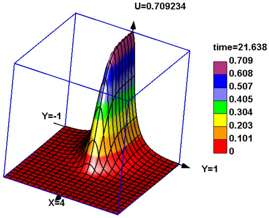
Figure 1.
A snapshot of solution of Equation (1) without immune response () and with a piece-wise constant genotype-dependent mortality . The cross section in the y-direction (genetic variable) shows a stationary distribution describing virus quasi-species. It has a maximum for some most frequent genotype, and it rapidly decays as the genotype moves away. This virus quasi-species progresses in the tissue (variable x).
We begin with a particular case where and the 2D problem can be reduced to some 1D problem depending on the x-variable (Section 2). It includes as a parameter the principal eigenvalue of some eigenvalue problem in the y-direction. This reduction allows us to carry out a detailed study of the dynamics of solutions. If , then the 1D problem depending on parameter provides an approximation of the 2D problem (Section 3 and Section 4). We use it to investigate the main features of infection progression and to determine how virus virulence and viral load depend on the width of genotype distribution, the strength of immune response, and the level of immunity (Section 5).
2. Wave Existence and Stability
We begin with a particular case , for which Equation (1) writes
We consider it in the whole , and we look for its solution in the form:
assuming that the initial condition satisfies a similar representation:
After the separation of variables
we obtain the equality
where is a constant. Hence,
Let be the principle eigenvalue of the operator
and the corresponding eigenfunction. Then, for all . Without loss of generality, we suppose that . We set . Then, satisfies this equation. We can now write Equation (6) as follows:
Thus, we have reduced 2D nonlocal Equation (4) to 1D local Equation (8). This reduction allows us to formulate the results on wave existence and stability.
Theorem 1.
Suppose that the function is continuous, and it has the limits at infinity, . Let be the principal eigenvalue of the operator such that . Then, solution of the Cauchy problem (4), (5) can be represented in the form , where satisfies of Equation (8), where , , is the eigenfunction of the operator corresponding to the principal eigenvalue, and for all .
The proof of the theorem is a consequence of the consideration above. We take into account that the principal eigenvalue of the operator is real and simple, and that the corresponding eigenfunction is positive if [38]. The assumption that the function has limits at infinity allows for an explicit determination of the essential spectrum, . If the limits do not exist, the essential spectrum cannot be explicitly determined but it can be estimated. The theorem remains applicable if the principal eigenvalue of the operator is greater than its upper bound. Let us also note that solution of problem (4), (5) is unique.
Reduction of Equation (4) to the 1D equation provided by Theorem 1 leads to the following result on the wave existence.
Theorem 2.
Under conditions of the previous theorem, let the function have a single positive zero , such that . Then, Equation (4) has travelling wave solutions , monotonically decreasing as a function of x, with the limits
Such solutions exist for all , where is a minimal speed, and they do not exist for .
The proof of the theorem follows from the corresponding results for the scalar reaction-diffusion equation in the monostable case [39]. According to the construction, travelling wave solutions of Equation (4) have the form , where , is a monotonically decreasing solution of the problem
An example of an analytical solution is constructed in the Appendix A.
Theorem 3.
As before, this theorem follows from the corresponding results for the 1D Equation [39] (see [40] and the references therein). Convergence here occurs in form and in speed. More general results and convergence to the waves with other speeds can be obtained.
3. 1D Problem Depending on the Eigenvalue
We consider the one-dimensional equation
where , and is the principal eigenvalue of the operator . For , this equation is obtained from the 2D problem by separation of variables. For , this reduction does not work, and we will use this equation as an approximation of the 2D problem. We set here and .
3.1. Properties of the Principal Eigenvalue
Consider the eigenvalue problem
on the whole real axis. In order to get a more complete information about the dependence of the principal eigenvalue on parameters, we consider a piece-wise constant function :
where and are some positive numbers. We will assume that (for ). Hence, the essential spectrum of problem (3) belongs to the left-half plane.
This eigenvalue problem can be solved analytically. Let us note that the eigenvalue with the maximal real part of this problem is negative. Set , . Then, satisfies the equation
Consider the minimal positive solution of this equation located at the first growing branch of tangent for . Since the right-hand side of Equation (12) is a decreasing function of , such solution exists for any and . The corresponding eigenfunction is given by the following expression:
Assuming that , we find :
Consider the limiting cases. If , then it follows from Equation (12) that . Hence , . If , then it follows from Equation (12) that and . From the second equality for , we conclude that . Hence, the maximum of the eigenfunction increases for small and decreases for large . Similar properties hold for a smoothed function .
3.2. Dynamics of 1D Waves
Dynamics of solutions of Equation (10) are studied for a wide class of functions (see [40] and the references therein). We will consider for certainty the function qualitatively describing the properties of immune response as a function of viral load. Here, are some non-negative numbers. Set , where , and is the principal eigenvalue of problem (11). The function vanishes at , and it has up to three positive zeros denoted in the growing order (Figure 2).
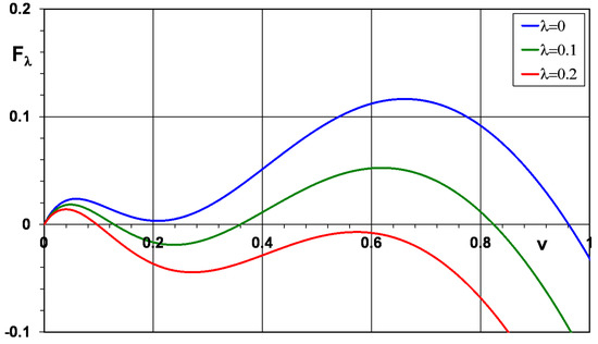
Figure 2.
Function for (upper curve), (middle curve), and (lower curve), , .
Equation (10) has a solution , that is, travelling wave with a speed c. For the function shown in Figure 2 (middle curve), there are three positive zeros and two different types of waves. The -waves are the waves with the limits and at infinity. This is so-called monostable case since the point is unstable with respect to the equation , and the point is stable. Such waves can be monotone as functions of x and non-monotone. The latter are unstable, and we will not consider them here. The monotone waves exist for all , where the minimal speed can be found by the formula since [39]. These waves are stable in a properly chosen space [40].
Let us recall that is determined by the principal eigenvalue of problem (11). It can be found from Equation (12) (). Therefore, we can determine the minimal speed of the monostable wave. Its dependence on is shown in Figure 3 (dashed curve).
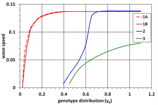
Figure 3.
Wave speed for the 1D Equation (10) (dashed line) and for the 2D Equation (1) (solid lines). Curves 1 and 3 correspond to the monostable and bistable waves, respectively, for the same values of parameters, and curve 2 shows the transition from the bistable wave to the monostable wave. The values of parameters are , , , (curves 1, 3, and dashed curve), and (curve 2).
The second wave is the -wave, which corresponds to the bistable case since both points and are stable as stationary points of equation . Such wave exists for a unique value of speed ; it is monotone as a function of x, and it is globally asymptotically stable. Its speed cannot be found analytically except for the case , which is reached if and only if the integral equals 0. The case of zero speed separates the cases where infection spreads in the tissue (positive speed) and where it does not spread (negative speed). We will discuss this question below.
Behavior of solutions of Equation (11) depends on the relation between the speeds and , and on the initial condition. For the function considered here, . In this case, there are two consecutive waves propagating one after another. The monostable -wave is followed by the -wave.
Denote the initial condition for Equation (11) by (Cauchy problem). For simplicity of presentation, suppose that it is a monotonically decreasing function with the limits at infinity. Then, for , the solution converges to the monostable -wave. We will restrict ourselves here to the convergence to the wave with the minimal speed that occurs, in particular, in the case where for all x that are sufficiently large. This case is most appropriate for applications and numerical simulations. If , then the solution converges to the system of two waves, monostable and bistable, propagating one after another with different speeds.
3.3. Dependence on
We discussed above behavior of solutions of Equation (11) for a fixed value of for which the function has three positive zeros. Let us now analyze how this behavior depends on the value of . Let us recall that depends on and decreases from to 0 as increases.
There are four critical values of that determine the behaviour of solutions (Table 1). The first one, , is such that for all if . In this case, the waves do not exist. For any (initial condition), the solution converges to 0. If , then the function has a positive zero . There exist monostable -waves, as described above.

Table 1.
Four critical values , determine the intervals of with different stationary points, waves, and their speeds.
If becomes less than the next critical value , then two more positive zeros and of the function appear. In this case, in addition to the monostable -waves, there is a bistable -wave with a negative speed. It becomes positive for . This critical value is determined by the equality . Let us note that the minimal speed increases with the decrease of for the monostable wave, similar to the single speed of the bistable wave. If , there is a system of two waves. As we discussed above, solution can converge either to the monostable wave or to the system of two waves depending on the initial condition. Zeros and merge for and disappear (Figure 2, upper curve). We return to the monostable case with the -waves.
3.4. Dependence on
Parameter characterizes the strength of immune response. Varying , we get the types of function similar to those considered above. Parameter determines the presence of immunity from the previous infection or vaccine. If , then is a stable stationary point. It is globally stable (for ) if for all positive v and locally stable if changes sign. In the latter case, there is a bistable -wave with a positive or negative depending on the sign of the integral .
4. 2D Wave Dynamics
In this section, we study dynamics of solutions of Equation (1) with . We will show that it correlates with the dynamics of solutions of 1D equation considered in the previous section.
4.1. Influence of the Genotype Distribution
Virus density distribution with respect to the genotype is determined by the function . We will vary the value of characterizing the width of this distribution, keeping constant. For sufficiently small values of , the trivial solution of Equation (1) is stable and wave propagation is not observed. For larger values of , the trivial solution loses its stability. Equation
has a positive solution , and there is a wave propagating in the x-direction with the limits at infinity (Figure 4, right). These limits are solutions of Equation (13). If we increase , the speed of this wave also increases (curves 1 in Figure 3).
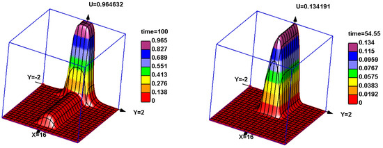
Figure 4.
Snapshots of solutions of Equation (1) with two different initial conditions and the same values of parameters. Two waves with different speeds propagate one after another for a sufficiently large initial condition (left). A faster monostable wave with a small amplitude is followed by a slower bistable wave with a large amplitude. If the initial condition is small enough, then only the fast monostable wave with a small amplitude is observed (right). The values of parameters: , , .
For , another solution is observed for the same values of parameters. It consists of two consecutive waves (Figure 4, left). A small amplitude wave is the same as in Figure 4, right (the scaling in the figures is different). It is followed by a high amplitude wave with a smaller speed. The presence of this second wave indicates the existence of another positive stationary solution of Equation (13), which is presumably stable. Therefore, we can expect that they are separated by an unstable solution that is not observed in the simulations. Thus, there exists a monstable -wave, and a bistable -wave. If the initial condition is small enough, the single small-amplitude wave propagates. If the initial condition is sufficiently large, then we observe the system of two waves. The speed of the bistable wave increases with (curve 2 in Figure 3).
4.2. Comparison with 1D Problem
We will now compare the 2D problem with the 1D problem, depending on the eigenvalue for the same and fixed values of parameters and varying . If is less than the first critical value, , then both solutions converge to the trivial solution. In both cases, we find . Let us recall that we determine the principal eigenvalue of problem (11) as a function of . These values of correspond to the first line in Table 1.
The monostable wave is observed for both problems for . The speeds of such waves are shown in Figure 3 (curve 1 and dashed curve). The wave speeds have a similar dependence on . We recall that this is the minimal speed of the 1D wave. In the case of 2D problem, we observe only one wave in numerical simulations. Therefore, strictly speaking, we cannot affirm that there are also waves with larger speeds. We can conjecture their existence by analogy with the 1D equation. This case corresponds to line 2 in Table 1.
In the next interval of values of , , along with the monostable wave, there exists a bistable wave with a negative speed. The speed becomes positive for (lines 3 and 4 in Table 1). For the chosen values of parameters, for the 2D problem and for the 1D problem. The latter is found analytically from the condition (Section 3). The speed of the bistable wave increases as a function of (Figure 3, curve 3).
4.3. Parameter Dependence
For the values of parameters considered above () and , the function has three positive zeros, , , and . If we increase , then zeros and approach each other, merge, and disappear. In this case, there is the only positive zero and the monostable -waves. This case is similar to the case of large considered above.
If we decrease , then zeros and merge and disappear. In this case, there is the only positive zero and the monostable -waves. This case was not considered above. Set and consider dynamics of 2D waves for different values of . The difference in comparison with the previous case () manifests itself in the behavior of the bistable wave for . Its speed rapidly grows and approaches the minimal speed of the monostable wave (Figure 3, curve 2). The bistable -wave and the monostable -wave disappear for , resulting in the emergence of the monostable -wave. In the 1D problem, this transition occurs for the same value of ().
Modelling and simulations presented above were carried out for . Function becomes qualitatively different if . The stationary solution of the equation becomes stable, and the function may not have positive zeros or have two of them (the degenerate case of merged zeros is not considered). In the first case, the trivial solution of the 1D problem is globally asymptotically stable. In the second case, this problem has a bistable -wave. The sign of its speed can be positive or negative depending on the other parameters. The transition between them is determined by the equality . Numerical simulations of the 2D problem also reveal the existence of a large amplitude -wave where , is a solution of Equation (13). Its speed changes sign for , for which ( and ), and the speed of the 1D is also close to zero.
Thus, dynamics of the 1D waves depending on the eigenvalue and of the 2D waves are similar to each other. They show the existence of the monostable and bistable waves, and of a monostable-bistable wave. Their parameter dependence is also analogous.
5. The Properties of Infection Progression
We will study in this section how infection spread in the tissue is influenced by the genotype distribution, the initial viral load, the strength of immune response, and the presence of immunity. We will characterize infection progression and immune response in terms of the parameters of the model.
- Genotype distribution. Virus genotype distribution depends on parameter characterizing the interval where the virus reproduction rate exceeds its natural mortality rate (without immune response), and on the mutation rate that determines the diffusion coefficient . These two parameters determine the principal eigenvalue of problem (11). Let us note that proportional decrease of and does not change , so that the results presented above are appropriate in a wide range of mutation rates.
- Strength of immune response. Adaptive immune response proceeds by clonal expansion of lymphocytes due to the interaction with antigens-presenting cells (macrophages, dendritic cells). For small viral loads, increase of the level of pathogens in the organism intensifies the immune response. Some viral infections can affect the functioning of lymphocytes by downregulating their proliferation and increasing their death (e.g., HIV, LCMV [41] but not coronavirus). Therefore, the function increases for small u and decreases for large u. Stronger immune response corresponds to a larger function . In modelling, we characterize the strength of immune response by the value of parameter .
- Immunity. Vaccination and previous infections can lead to the appearance of antibodies and memory cells responding to a new antigen. This response can be attenuated by the reduced affinity to the antigen of the immunity mediators (antibodies, T cell receptors). Immunity slows down infection progression and accelerates clonal expansion of immune cells. We model the presence of immunity by the coefficient . If it is positive, then immune response starts from some positive value under the introduction of antigen, . Infection-free equilibrium becomes stable for sufficiently narrow genotype distribution , and infection is eliminated unless the initial viral load is sufficiently large to cause its persistent progression.
- Viral load. The level of infection in the tissue determines the severity of symptoms and the intensity of infection transmission to other individuals. Viral load is determined by all factors presented in the previous paragraphs. In modelling, it corresponds to the virus density distribution after the wave propagation.
- Virus virulence. Virus virulence is characterized by its spreading rate. In modelling, it is determined by the coefficient k in Equation (1). In the absence of immune response, it is related to the minimal speed of the monostable wave . Multiplicity of infection tests in cell culture [42] characterize the virulence of infection by the speed of viral plaque growth, that is, by the wave speed. We will also characterize the virulence of infection by the wave speed in the presence of immune response.
We will determine how viral load and virulence depend on the strength of immune response, the level of immunity, and the width of the genotype distribution. Since the 2D problem can be approximate with the 1D problem depending on eigenvalue, we will use the latter for the investigation of infection progression. It will allow us to obtain a relatively simple analytical description of its main features.
If the disease-free equilibrium is stable, then infection does not develop for sufficiently small initial viral loads and solution uniformly converges to 0. If it is unstable, then a positive disease equilibrium appears and there is a wave of infection propagation. Figure 5 shows the stability region depending on the width of genotype distribution (parameter ) and on the level of immunity (coefficient ). If the latter is large enough, then the disease free equilibrium is stable. In the 1D problem, the stability boundary is determined by the function , where is the principal eigenvalue of problem (11) (up to sign). The stability boundary for the 1D problem is compared with the result of numerical simulation of the 2D problem. Let us note that the disease-free equilibrium can be globally stable or stable only to small perturbations. In the second case, there are two positive stationary points and a bistable wave describing disease progression for a sufficiently large initial viral load. We will return to this question below.
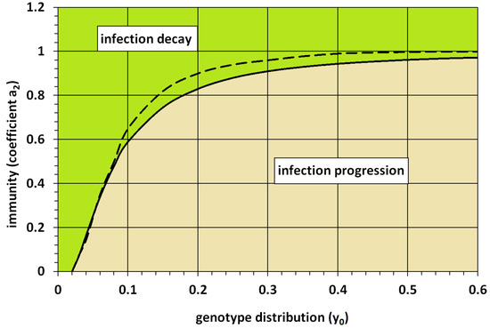
Figure 5.
The critical value of immunity (coefficient ) is shown as a function of the width of the genotype distribution (). If the value of immunity exceeds the critical value, then infection is eliminated. Otherwise, it progresses. Solid line represents the results of 2D simulations, and dashed line is given by the formula for the 1D problem. The values of parameters: , , and .
Next, we study how the virulence of infection depends on the level of immunity. We determine the virulence as the minimal speed of the monostable wave, . For a fixed width of genotype distribution, it becomes a function of , that is, a function of immune memory protection in the absence of pathogen. As it can be expected, the virulence of infection decreases with the increase of immunity level (Figure 6). Infection does not develop if immunity level exceeds the critical value where the curve crosses the x-axis.
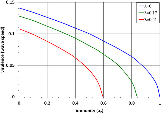
Figure 6.
Dependence of virulence (wave speed) on immunity (). The minimal wave speed is found by the formula for the 1D problem. The upper curve corresponds to (limit of large ), the middle curve to (), and the lower curve to (). The values of parameters: , , and .
Viral load is an independent characteristic with respect to virus virulence. We determine it as the maximal level of virus concentration during infection progression in the tissue. Hence, in the 1D problem, it corresponds to positive zeros of the function . There are two essentially different cases presented in Figure 7. Curve 1 corresponds to the bistable case with two positive zeros and ; ; and a bistable -wave. The value is on the lower branch of this curve, and on the upper branch. Let us recall that the initial condition in the 1D problem considered on the whole axis is a function with the limits , . Here, is the initial viral load. If it exceeds , then the solution converges to the bistable wave with the maximal value (viral load) . If , then the solution uniformly converges to 0 and infection is eliminated. If the strength of immune response (parameter ) is larger then some critical value, then there are no positive zeros of the function . The disease-free equilibrium is globally stable, and infection is eliminated for any initial viral load.
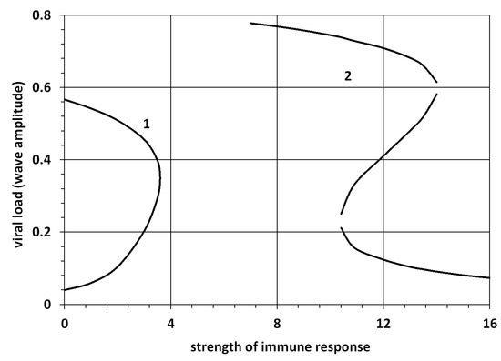
Figure 7.
Dependence of the viral load (wave amplitude) on the strength of immune response () for the 1D problem. The wave amplitude is found as a solution of the equation . The values of parameters: , , Curve 1: , (). Curve 2: , ().
The second curve corresponds to the case with up to three positive zeros of the function and the existence of either monostable or monostable-bistable waves. The lower branch of the curve shows the value of , the middle branch , and the upper branch . For a weak immune response, there is only one positive solution at the upper branch and the corresponding large amplitude monostable -wave. For a strong immune response, there is the monostable -wave with small amplitude. For the intermediate values, there are three positive zeros and the monostable-bistable system of waves, where the monostable -wave is followed by the bistable -wave with a smaller speed. In this case, if the initial viral load is small enough, then the final viral load remains small. If the initial viral load is sufficiently large, then the viral load proceeds in two consecutive steps, first a small one, then a large one. In terms of disease progression, a mild form of the disease is followed by a severe form.
6. Discussion
Viral infection development in the tissues of the host organism depends on many factors determined by the pathogen and by the immune response to the infection. In this work, we study the influence of virus genotype distribution on spatial infection spreading.
6.1. Model
The model suggested in this work is a generalization of the 1D model introduced in [34] for the infection spreading in the tissue. This 1D model describes spatiotemporal virus distribution taking into account its random motion, reproduction, and elimination due to the immune response.
In order to study virus density distribution with respect to its genotype, we need to introduce its genotypical characteristic as a continuous variable. The simplest way to do it is to consider a sequence of consecutive mutations and the corresponding genotypes denoted by . Transition from the genotype to the genotype occurs due to one of the mutations of this sequence. Let be the virus density corresponding to the genotype . Assuming that all mutations are reversible and have the same rate, we obtain the following equations for :
It is a discrete version of the diffusion equation. Diffusion coefficient depends on the probability of mutations and on the characteristic space interval . The half-length of the admissible interval can be represented as , where k is the number of mutations from the most frequent genotype to the end of viability interval.
The ratio , independent of , determines the principle eigenvalue of the operator . Therefore, solutions are characterized by the value and not by the individual parameters and .
The combination of the space variable x and the genotype variable y allows us to study the influence of genotype distribution on infection spreading. The method developed in this work is also applicable for the equation with time delay.
6.2. Method and Results
The method developed in this work implies the reduction of the 2D problem to a 1D problem in the x-direction and to some eigenvalue problem in the y-direction. In a particular case, this reduction is exact. It allows us to study the existence and stability of travelling waves. The case with time delay, though not considered in this work, can be studied by the same method. Dynamics of 1D solutions with time delay is investigated in [34,43].
In the general case, the exact reduction of the 2D problem to the 1D problem is not possible. We consider the 1D problem depending on the eigenvalue as an approximation of the 2D problem. In some limiting cases, this approximation might be possible to justify by more rigourous mathematical considerations but this question is beyond the scope of this work. Numerical simulations of the 2D problem are in a good agreement with the analytical results for the 1D problem.
We use the 1D problem depending on the eigenvalue in order to study the progression of viral infection. Virus virulence (wave speed) and viral load (wave amplitude) are determined by the width of the genotype distribution (), strength of immune response (), level of immunity (), and the initial viral load (initial condition). Detailed characterization of infection progression is presented in the previous section. Let us mention here that the increase of the width of the genotype distribution increases virus virulence and viral load.
6.3. Limitations and Perspectives
We consider a simplified model of infection development where immune response is reduced to a function describing the immune cell concentration depending on virus density. This model follows from a more detailed model due to a quasi-stationary approximation [36]. Time delay characterizing the duration of the clonal expansion of immune cells is not taken into account in order to simplify the presentation and to concentrate on other aspects of the problem. The dependence of the virus density distribution on the genotype variable is considered in the simplest approximation of reversible consecutive mutations. Finally, the developed model provides the tool for comprehensive analysis and evaluation of the link between the viral evolution and immune escape from the immunodominant CD8+ T cell responses [44]. More complex mutation patterns can be considered.
Author Contributions
Investigation, V.V.; Methodology, G.B.; Software, N.B. All authors have read and agreed to the published version of the manuscript.
Funding
The research was funded by the Russian Science Foundation (Grant no. 18-11-00171). G.B. was partly supported by Moscow Center of Fundamental and Applied Mathematics (agreement with the Ministry of Education and Science of the Russian Federation No. 075-15-2019-1624).
Institutional Review Board Statement
Not applicable.
Informed Consent Statement
Not applicable.
Data Availability Statement
Not applicable.
Conflicts of Interest
The authors declare no conflict of interest.
Appendix A. Analytical Solution for Nonlocal Equation
We will construct here the analytical solution of the equation
where c is the speed of the wave, and
In what follows we set . We look for the solution of Equation (A1) in the form: , where for and for . Substituting these expressions into the equation, we obtain for :
where , . Separating the variables in the last equation, we have
The left-hand side of this equality depends only on x, the next expression depends only on y. Therefore, both of them equal some constant . Hence,
Similarly,
We set
such that satisfies the same equation in (A3) and in (A4). Next, we suppose that and . Then
where , and are arbitrary constants. From the conditions , (similar conditions at ),
Dividing the second equation in (A6) by the first one and taking into account (A5), we obtain the equation with respect to :
This equation has at least one solution for any . It can have more than one solution for sufficiently large. Thus,
where a is an arbitrary positive constant, is a solution of Equation (A7), ,
Equation (A10) is similar to the KPP equation. It has a monotonically decreasing solution if for all , where .
From the first equation in (A5) we obtain . Hence, . This solution does not depend on the arbitrary constant a. The following theorem is proved.
Theorem A1.
Suppose that is a solution of Equation (A7), . Then, Equation (A1) has a solution for all , where is a solution of problem (A10), (A11), and are determined by expressions (A8), (A9). Its second derivative with respect to x is continuous for all , its second derivative with respect to y is continuous for all except for .
References
- Biebricher, C.K.; Eigen, M. What is a quasispecies? Curr. Top. Microbiol. Immunol. 2006, 299, 1–31. [Google Scholar]
- Domingo, E.; Perales, C. Viral quasispecies. PLoS Genet. 2019, 15, e1008271. [Google Scholar] [CrossRef] [Green Version]
- Goodenow, M.; Huet, T.; Saurin, W.; Kwok, S.; Sninsky, J.; Wain-Hobson, S. HIV-1 isolates are rapidly evolving quasispecies: Evidence for viral mixtures and preferred nucleotide substitutions. J. Acquir. Immune Defic. Syndr. 1989, 2, 344–352. [Google Scholar]
- Holland, J.J.; De La Torre, J.C.; Steinhauer, D.A. RNA virus populations as quasispecies. Curr. Top. Microbiol. Immunol. 1992, 176, 1–20. [Google Scholar] [PubMed]
- Meyerhans, A.; Cheynier, R.; Albert, J.; Seth, M.; Kwok, S.; Sninsky, J.; Morfeldt-Manson, L.; Asjo, B.; Wain-Hobson, S. Temporal fluctuations in HIV quasispecies in vivo are not reflected by sequential HIV isolations. Cell 1989, 58, 901–910. [Google Scholar] [CrossRef]
- Poirier, E.Z.; Vignuzzi, M. Virus population dynamics during infection. Curr. Opin. Virol. 2017, 23, 82–87. [Google Scholar] [CrossRef]
- Kautz, T.F.; Forrester, N.L. RNA Virus Fidelity Mutants: A Useful Tool for Evolutionary Biology or a Complex Challenge? Viruses 2018, 10, 600. [Google Scholar] [CrossRef] [Green Version]
- Karamitros, T.; Papadopoulou, G.; Bousali, M.; Mexias, A.; Tsiodras, S.; Mentis, A. SARS-CoV-2 exhibits intra-host genomic plasticity and low-frequency polymorphic quasispecies. J. Clin. Virol. 2020, 131, 104585. [Google Scholar] [CrossRef]
- Keele, B.H.; Giorgi, E.E.; Salazar-Gonzalez, J.F.; Decker, J.M.; Pham, K.T.; Salazar, M.G.; Sun, C.; Grayson, T.; Wang, S.; Li, H.; et al. Identication and characterization of transmitted and early founder virus envelopes in primary HIV-1 infection. Proc. Natl. Acad. Sci. USA 2008, 105, 7552–7557. [Google Scholar] [CrossRef] [Green Version]
- Plikat, U.; Nieselt-Struwe, K.; Meyerhans, A. Genetic drift can dominate short-term human immunodeficiency virus type 1 nef quasispecies evolution in vivo. J. Virol. 1997, 71, 4233–4240. [Google Scholar] [CrossRef] [Green Version]
- Mattenberger, F.; Vila-Nistal, M.; Geller, R. Increased RNA virus population diversity improves adaptability. Sci. Rep. 2021, 11, 6824. [Google Scholar] [CrossRef] [PubMed]
- Jary, A.; Leducq, V.; Malet, I.; Marot, S.; Klement-Frutos, E.; Teyssou, E.; Soulié, C.; Abdi, B.; Wirden, M.; Pourcher, V.; et al. Evolution of viral quasispecies during SARS-CoV-2 infection. Clin. Microbiol. Infect. 2020, 26, 1560.e1–1560.e4. [Google Scholar] [CrossRef] [PubMed]
- Vignuzzi, M.; Stone, J.K.; Arnold, J.J.; Cameron, C.E.; Andino, R. Quasispecies diversity determines pathogenesis through cooperative interactions in a viral population. Nature 2006, 439, 344–348. [Google Scholar] [CrossRef]
- Karakasiliotis, I.; Lagopati, N.; Evangelou, K.; Gorgoulis, V.G. Cellular senescence as a source of SARS-CoV-2 quasispecies. FEBS J. 2021; Epub ahead of print. [Google Scholar] [CrossRef]
- Sun, F.; Wang, X.; Tan, S.; Dan, Y.; Lu, Y.; Zhang, J.; Xu, J.; Tan, Z.; Xiang, X.; Zhou, Y.; et al. SARS-CoV-2 Quasispecies Provides an Advantage Mutation Pool for the Epidemic Variants. Microbiol. Spectr. 2021, 9, e0026121. [Google Scholar] [CrossRef]
- Collier, D.A.; Monit, C.; Gupta, R.K. The Impact of HIV-1 drug escape on the global treatment landscape. Cell Host Microbe 2019, 26, 48–60. [Google Scholar] [CrossRef]
- Esposito, I.; Trinks, J.; Soriano, V. Hepatitis C virus resistance to the new direct-acting antivirals. Expert Opin. Drug Metab. Toxicol. 2016, 12, 1197–1209. [Google Scholar] [CrossRef] [PubMed]
- Kiepiela, P.; Leslie, A.J.; Honeyborne, I.; Ramduth, D.; Thobakgale, C.; Chetty, S.; Rathnavalu, P.; Moore, C.; Pfaerott, K.J.; Hilton, L. Dominant inuence of HLA-B in mediating the potential co-evolution of HIV and HLA. Nature 2004, 432, 769–775. [Google Scholar] [CrossRef]
- Illingworth, C.J.R.; Raghwani, J.; Serwadda, D.; Sewankambo, N.K.; Robb, M.L.; Eller, M.A.; Redd, A.R.; Quinn, T.C.; Lythgoe, K.A. A de novo approach to inferring within-host fitness effects during untreated HIV-1 infection. PLoS Pathog. 2020, 16, e1008171. [Google Scholar] [CrossRef] [PubMed]
- Phillips, R.E.; Rowland-Jones, S.; Nixon, D.F.; Gotch, F.M.; Edwards, J.P.; Ogunlesi, A.O.; Elvin, J.G.; Rothbard, J.A.; Bangham, C.R.; Rizza, C.R.; et al. Human immunodeficiency virus genetic variation that can escape cytotoxic T cell recognition. Nature 1991, 354, 453–459. [Google Scholar] [CrossRef]
- Larder, B.A.; Kemp, S.D. Multiple mutations in HIV-1 reverse transcriptase confer high-level resistance to zidovudine (AZT). Science 1989, 246, 1155–1158. [Google Scholar] [CrossRef]
- McMichael, A.J.; Borrow, P.; Tomaras, G.D.; Goonetilleke, N.; Haynes, B.F. The immune response during acute HIV-1 infection: Clues for vaccine development. Nat. Rev. Immunol. 2010, 10, 11–23. [Google Scholar] [CrossRef]
- Yang, Y.; Ganusov, V.V. Kinetics of HIV-Specific CTL Responses Plays a Minimal Role in Determining HIV Escape Dynamics. Front. Immunol. 2018, 9, 140. [Google Scholar] [CrossRef] [PubMed] [Green Version]
- Conway, J.M.; Ribeiro, R.M. Modeling the immune response to HIV infection. Curr. Opin. Syst. Biol. 2018, 12, 61–69. [Google Scholar] [CrossRef]
- Bocharov, G.; Chereshnev, V.; Gainova, I.; Bazhan, S.; Bachmetyev, B.; Argilaguet, J.; Martinez, J.; Meyerhans, A. Human Immunodeficiency Virus Infection: From Biological Observations to Mechanistic Mathematical Modelling. Math. Model. Nat. Phenom. 2012, 7, 78–104. [Google Scholar] [CrossRef]
- Haas, G.; Plikat, U.; Debré, P.; Lucchiari, M.; Katlama, C.; Dudoit, Y.; Bonduelle, O.; Bauer, M.; Ihlenfeldt, H.G.; Jung, G.; et al. Dynamics of viral variants in HIV-1 Nef and specific cytotoxic T lymphocytes in vivo. J. Immunol. 1996, 157, 4212–4221. [Google Scholar]
- Ganusov, V.V.; Goonetilleke, N.; Liu, M.K.; Ferrari, G.; Shaw, G.M.; McMichael, A.J.; Borrow, P.; Korber, B.T.; Perelson, A.S. Fitness costs and diversity of the cytotoxic T lymphocyte (CTL) response determine the rate of CTL escape during acute and chronic phases of HIV infection. J. Virol. 2011, 85, 10518–10528. [Google Scholar] [CrossRef] [Green Version]
- Turnbull, E.L.; Wong, M.; Wang, S.; Wei, X.; Jones, N.A.; Conrod, K.E.; Aldam, D.; Turner, J.; Pellegrino, P.; Keele, B.F.; et al. Kinetics of expansion of epitope-specific T cell responses during primary HIV-1 infection. J. Immunol. 2009, 182, 7131–7145. [Google Scholar] [CrossRef] [Green Version]
- Ganusov, V.V.; Neher, R.A.; Perelson, A.S. Mathematical modeling of escape of HIV from cytotoxic T lymphocyte responses. J. Stat. Mech. 2013, 2013, P01010. [Google Scholar] [CrossRef] [PubMed]
- Bocharov, G.A.; Ford, N.J.; Edwards, J.; Breinig, T.; Wain-Hobson, S.; Meyerhans, S.A. A genetic algorithm approach to simulating human immunodeficiency virus evolution reveals the strong impact of multiply infected cells and recombination. J. Gen. Virol. 2005, 86, 3109–3118. [Google Scholar] [CrossRef] [PubMed]
- Merleau, N.S.C.; Pénisson, S.; Gerrish, P.J.; Elena, S.F.; Smerlak, M. Why are viral genomes so fragile? The bottleneck hypothesis. PLoS Comput. Biol. 2021, 17, e1009128. [Google Scholar] [CrossRef]
- Swanstrom, R.; Coffin, J. HIV-1 pathogenesis: The virus. Cold Spring Harb. Perspect. Med. 2012, 2, a007443. [Google Scholar] [CrossRef] [Green Version]
- Bellomo, N.; Painter, K.J.; Tao, Y.; Winkler, M. Occurrence vs. Absence of Taxis-Driven Instabilities in a May-Nowak Model for Virus Infection. SIAM J. Appl. Math. 2019, 79, 1990–2010. [Google Scholar] [CrossRef]
- Bocharov, G.; Meyerhans, A.; Bessonov, N.; Trofimchuk, S.; Volpert, V. Spatiotemporal dynamics of virus infection spreading in tissues. PLoS ONE 2016, 11, e0168576. [Google Scholar] [CrossRef] [PubMed]
- Bessonov, N.; Bocharov, G.; Meyerhans, A.; Popov, V.; Volpert, V. Nonlocal reaction-diffusion model of viral evolution: Emergence of virus strains. Mathematics 2020, 8, 117. [Google Scholar] [CrossRef] [Green Version]
- Bocharov, G.; Meyerhans, A.; Bessonov, N.; Trofimchuk, S.; Volpert, V. Modelling the dynamics of virus infection and immune response in space and time. Int. J. Parallel Emergent Distrib. Syst. 2019, 34, 341–355. [Google Scholar] [CrossRef] [Green Version]
- Bessonov, N.; Bocharov, G.A.; Leon, C.; Popov, V.; Volpert, V. Genotype-dependent virus distribution and competition of virus strains. Math. Mech. Complex Syst. 2020, 8, 101–126. [Google Scholar] [CrossRef]
- Volpert, A.; Volpert, V. Spectrum of ellipticoperators and stability of travelling waves. Asymptot. Anal. 2000, 23, 111–134. [Google Scholar]
- Kolmogorov, A.N.; Petrovskiı, I.G.; Piskunov, N.S. Etude de l’équation de la chaleur avec croissance de la quantité de matière et son application à un problème biologique. Bull. Moskov. Gos. Univ. Mat. Mekh. 1937, 1, 1–25. [Google Scholar]
- Volpert, A.; Volpert, V.; Volpert, V. Traveling Wave Solutions of Parabolic Systems; Translation of Mathematical Monographs; American Mathematical Society: Providence, RI, USA, 1994; Volume 140. [Google Scholar]
- Bocharov, G.; Volpert, V.; Ludewig, B.; Meyerhans, A. Mathematical Immunology of Virus Infections; Springer: Berlin/Heidelberg, Germany, 2018. [Google Scholar]
- Holder, B.P.; Simon, P.; Liao, L.E.; Abed, Y.; Bouhy, X.; Beauchemin, C.A.A.; Boivin, G. Assessing the In Vitro Fitness of an Oseltamivir-Resistant Seasonal A/H1N1 Influenza Strain Using a Mathematical Model. PLoS ONE 2011, 6, e14767. [Google Scholar] [CrossRef] [Green Version]
- Bessonov, N.; Bocharov, G.; Touaoula, T.M.; Trofimchuk, S.; Volpert, V. Delay reaction-diffusion equation for infection dynamics. Discret. Contin. Dyn. Syst. B 2019, 24, 2073. [Google Scholar] [CrossRef] [Green Version]
- Henn, M.R.; Boutwell, C.L.; Charlebois, P.; Lennon, N.J.; Power, K.A.; Macalalad, A.R.; Berlin, A.M.; Malboeuf, C.M.; Ryan, E.M.; Gnerre, S.; et al. Whole Genome Deep Sequencing of HIV-1 Reveals the Impact of Early Minor Variants Upon Immune Recognition During Acute Infection. PLoS Pathog. 2012, 8, e1002529. [Google Scholar] [CrossRef] [PubMed] [Green Version]
Publisher’s Note: MDPI stays neutral with regard to jurisdictional claims in published maps and institutional affiliations. |
© 2021 by the authors. Licensee MDPI, Basel, Switzerland. This article is an open access article distributed under the terms and conditions of the Creative Commons Attribution (CC BY) license (https://creativecommons.org/licenses/by/4.0/).