A Two-Step Polynomial and Nonlinear Growth Approach for Modeling COVID-19 Cases in Mexico

Abstract

Since December 2019, the novel coronavirus (SARS-CoV-2) and its associated illness COVID-19 have rapidly spread worldwide. The Mexican government has implemented public safety measures to minimize the spread of the virus. In this paper, we used statistical models in two stages to estimate the total number of coronavirus (COVID-19) cases per day at the state and national levels in Mexico. In this paper, we propose two types of models. First, a polynomial model of the growth for the first part of the outbreak until the inflection point of the pandemic curve and then a second nonlinear growth model used to estimate the middle and the end of the outbreak. Model selection was performed using Vuong’s test. The proposed models showed overall fit similar to predictive models (e.g., time series and machine learning); however, the interpretation of parameters is simpler for decisionmakers, and the residuals follow the expected distribution when fitting the models without autocorrelation being an issue.

1. Introduction

The world is currently experiencing a pandemic caused by the novel coronavirus, formally named COVID-19 by the World Health Organization (WHO). Development of a vaccine and antiviral drugs to treat COVID-19 is still ongoing, resulting in hospitalization and intensive care unit management as the only option in treating COVID-19. Thus, there is a dire need for research on modeling the outbreak of COVID-19 to help officials in their decision-making processes regarding interventions and allocation of resources [1]. At the time this manuscript was being written, the pandemic was ongoing, and most of the epidemiological models developed focused on short-term predictions, identifying the daily peak of COVID-19 cases, predicting the duration of the pandemic, and estimating the possible impact of the measures implemented for minimizing exposure to the virus and decrease the fatality rate [2,3,4,5,6,7,8,9,10].

As of 24 September 2020, the cumulative number of COVID-19 cases in Mexico was reported as 715,457 [5], and 32,245,122 cases were reported worldwide [11]. Thus, the main objective of this paper was to model the total number of COVID-19 cases per day at the national and the state level in Mexico while simultaneously providing straightforward information to decisionmakers; additionally, we sought to determine which model provides the most stable short-term predictions. 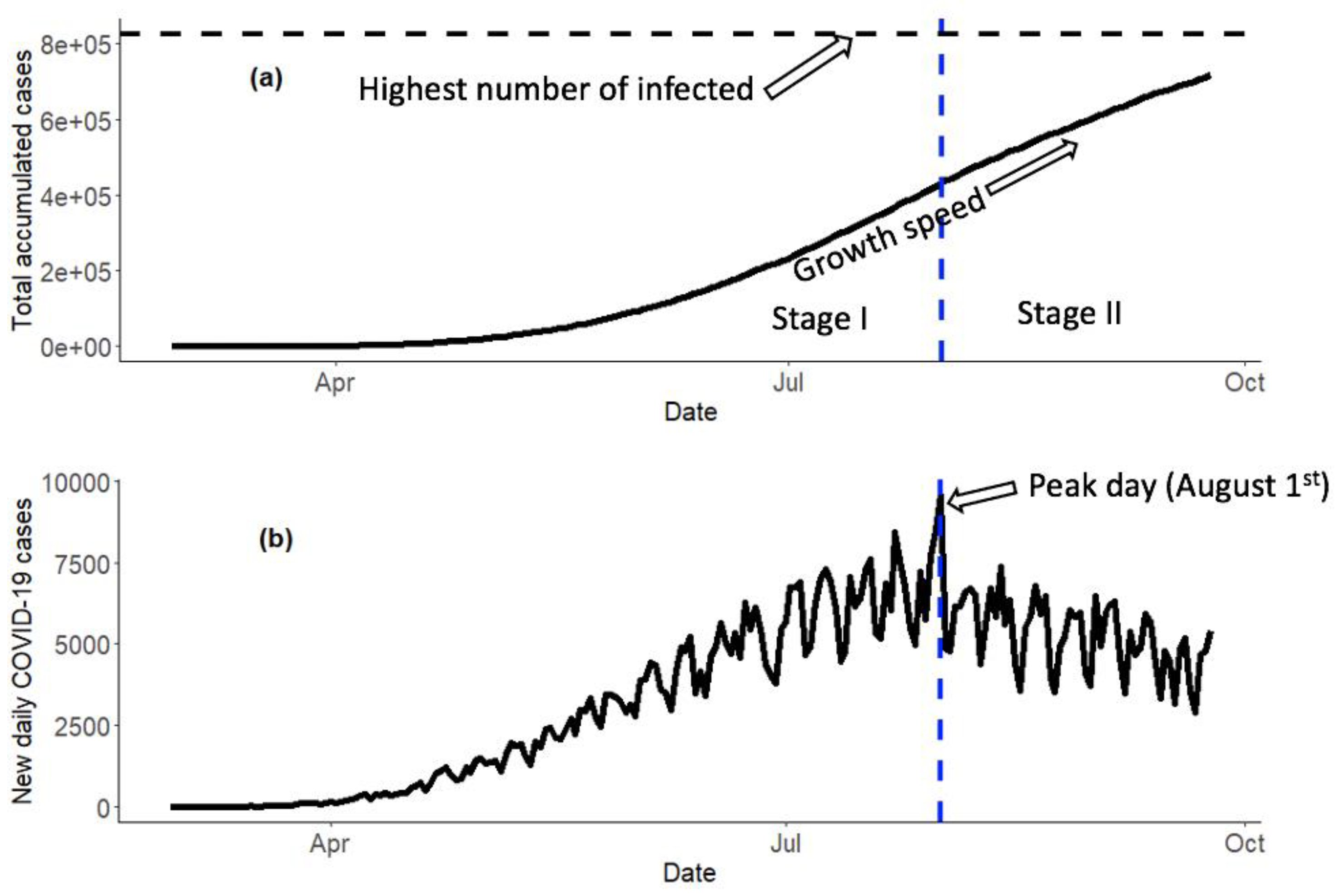Figure 1 shows the accumulated cases and new cases at the national level in Mexico. This figure shows the first wave peak of the pandemic until the data cut-off of 24 September. Until the 24 September date, only a single wave of infections had been observed (on 1 August). The models developed in this research facilitate the obtaining of information to support decisionmakers in the strategic planning activities of the Mexican states, metropolitan areas, municipalities, or cities with high population density. Mexican officials can use these models to aid in the management process involving the needs and resources of the health services such as available hospital beds, intensive care units, and respirators, as well as personal protective equipment (PPE) for health personnel. For decisionmakers, such as public health officials, having access to daily and permanent monitoring at the center of the pandemic allows them to anticipate the purchase of the necessary medical equipment in advance. Further, the authors would like to share these models so that officials and statisticians outside of Mexico can make use of them for their own decision-making procedures during the length of the COVID-19 pandemic. The proposed methodology in this paper can easily be applied to COVID-19 worldwide.

In this work we refer to 1–2–3 models as two-step models due to the method used to estimate their parameters [12]. The method is performed in two steps that will combine information from time series models with non-linear growth models and polynomial models. The two-step estimation is a process, also known as the Cochrane–Orcutt procedure, which is defined as:

“A two-step estimation of a linear regression model with first-order serial correlation in the errors. In the first step the first-order autocorrelation coefficient is estimated using the ordinary least squares residuals from the main regression equation. In the second step this estimate is used to rescale the variables so that the regression in terms of rescaled variables has no serial correlation in the errors. This is an example of feasible generalized least squares estimation” [13].

Several machine learning (ML) and artificial intelligence (AI) models have demonstrated acceptable performance in the modeling of the COVID-19 pandemic; our proposed methodology meets this expectation in addition to a simple estimation of the parameters. Unlike the susceptible–infected–recovered–deceased (SIRD) models, the proposed models do not require setting or assuming the value of any parameter to obtain the estimates [14,15]. Finally, another advantage of our models is the interpretability of their parameters, that is, estimates of some parameters directly linked to the pandemic can be obtained.

The article is structured as follows: In Section 2, we summarize the most relevant literature regarding the modeling of the COVID-19 pandemic. Next, in Section 3, the data used are presented and the proposed methodology is described. Section 4 shows the main results of the investigation. Finally, in Section 5, the main conclusions are presented, and the limitations of this research are discussed.

2. Literature Review

Research exists with data-driven approaches such as autoregressive (AR) and autoregressive integrated moving average (ARIMA), ranging from simple models (exponential smoothing) to more complex models such as ARIMAX, ARCH, GARCH, and ARFIRMA [2,7,8,10,16,17]. For example, we used an ARIMA model with data compiled by Johns Hopkins University to predict models for the daily confirmed cases in countries where the pandemic was peaking and to predict and anticipate the resources of the healthcare systems [18]. Unfortunately, these data-driven models fail to fit the data and often lack accuracy [6,19]. Additionally, the parameters of these models cannot be interpreted according to the reality of the pandemic. This interpretability barrier causes statisticians and officials to make their decisions on the basis of predictive models instead of the peak of the pandemic or the growth of the pandemic. A useful model for policy and public health decisionmakers during the COVID-19 pandemic would be a model that, in addition to obtaining accurate predictions, provides insights on the evolution or current behavior of the pandemic. Another approach is real-time forecasting using a generalized logistic growth model. This method has been previously used in China to generate short-term forecasting of COVID-19 cases [20,21], as well as with data from Canada, France, India, South Korea, and the UK to forecast daily cases [22,23]. These models are incredibly useful in that they provide information on the current state of the pandemic. However, in this study, we had two aims regarding logistic growth models: (1) to demonstrate that their assumption of independence of and (2) that their modeling performance at the earlier stages of the pandemic is not optimal but can be improved by the incorporation of an autoregressive component [4,9].

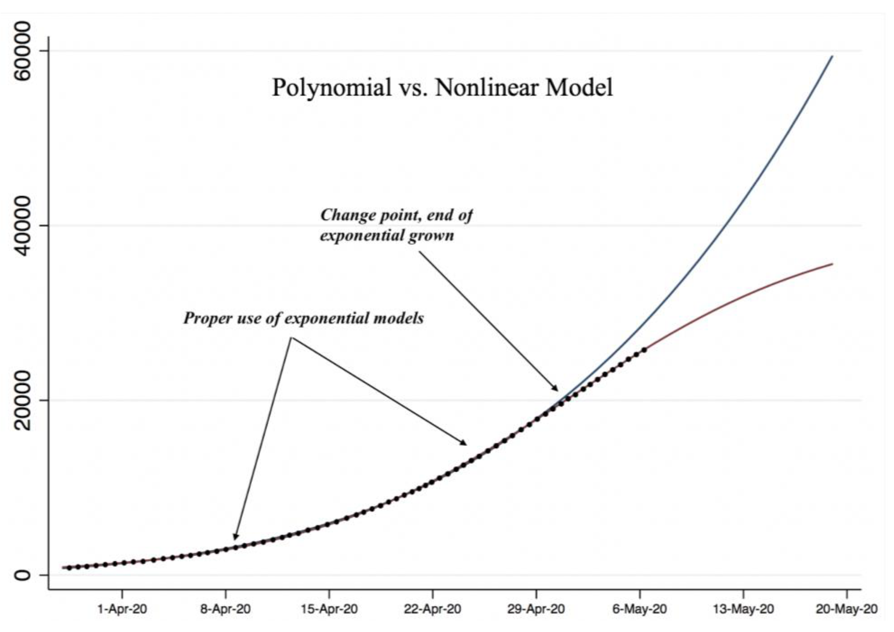
The models used in this paper are based on statistical linear models, classic time series, and restricted growth—called limited growth or nonlinear growth models [1,2,3,13,24]—as well as real-time forecasting using generalized logistic growth model [4,25]. In this paper, we propose estimations in two stages of the pandemic utilizing polynomial and nonlinear growth functions while incorporating an autoregressive component with the purpose of meeting the assumption of independence of residuals. First, we propose using a polynomial function estimated using the Prais–Winsten methodology to estimate the first stage of the pandemic (when exponential growth of COVID-19 cases was observed). Our rationale for choosing a third-degree polynomial model was the following: under certain scenarios: it can be converted into an increasing monotonic function, which is essential when modeling the total of accumulated cases; the degree is three since it shows simplicity with respect to higher-order polynomials; and when its behavior is observed, it has the shape of an “S”.

Next, in the second stage of the pandemic (when the peak of COVID-19 cases was reached), we propose utilization of nonlinear growth functions, logistic, and Gompertz in order to predict the total cumulative number of cases and the growth rate of the spread of COVID-19. In each of the models estimated before and after the peak of the pandemic, at the second stage of modeling, we added an autoregressive component of order one (AR (1)) to compare the results to the models that do not account for the violation of independence of residuals. This approach has been successfully used to model plant and animal growth where measuring the same unit can lead to violation of independence of residuals [9,25,26]. Next, we selected the best estimate equation to model the pandemic by using Vuong’s test criterion [27]. We anticipated the proposed model to have good performance similar to neural networks (NN) or support vector machines (SVM). A disadvantage of NN is that it is difficult to generate a day-to-day prediction in addition to finding the growth rate and finding the maximum number of cases. These are not a problem for the functions we propose. Furthermore, artificial intelligence (AI) has been used to identify, track, and forecast COVID-19 cases. However, AI models are difficult to interpret—the process by which they arrive at a decision is often referred to as a “black box” due to the complexity in understanding how AI models arrive at certain conclusions [28]. The complex interpretation may create a barrier for decisionmakers looking for straightforward solutions in the middle of a pandemic. Moreover, we anticipate our proposed modeling of the pandemic will meet the assumption of independence of residuals. In contrast to NN, our proposed model can provide predictions and will facilitate interpreting parameters such as the highest number of infected individuals, growth speed, the initial number of infected individuals, and the autoregressive parameter to measure the lag in reporting the new daily cases of infections.

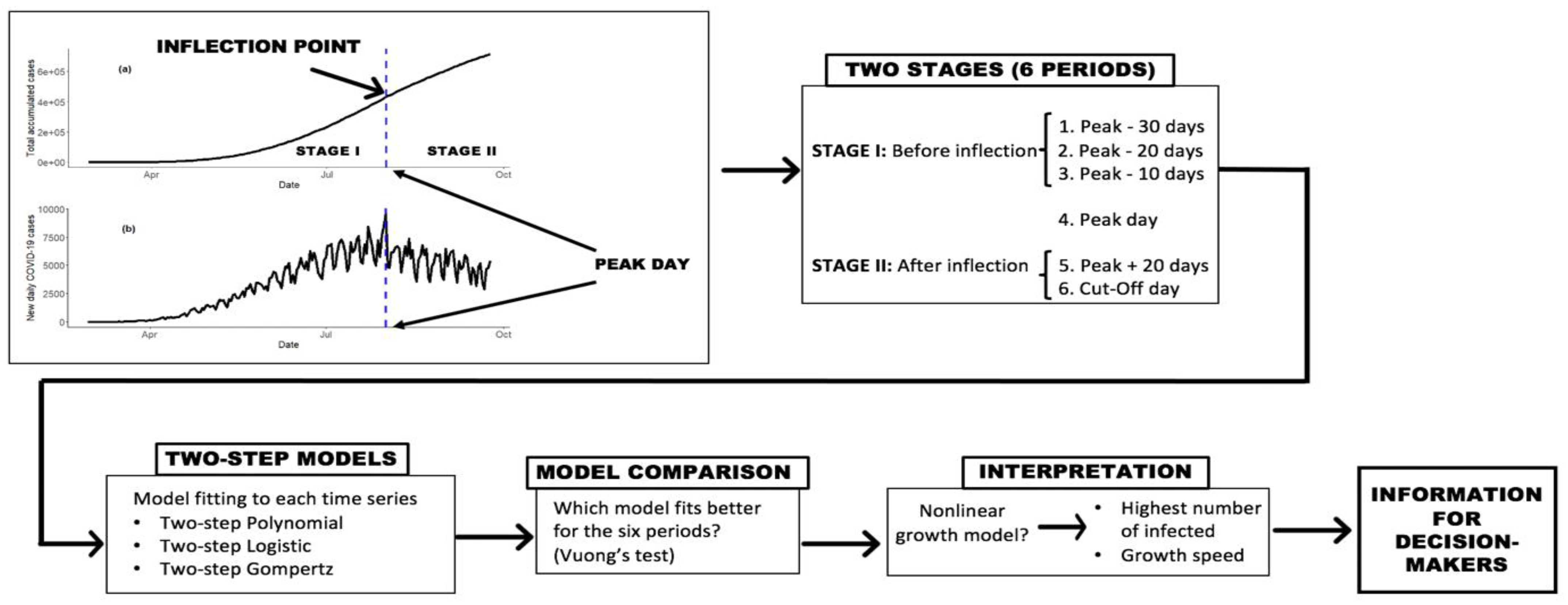
In summary, we present these two models (polynomial and nonlinear growth models) because of ease of interpretation for non-statistician decisionmakers, their stable and useful predictions while accounting for the autocorrelation of the data, and their insights regarding the current state of the pandemic. Therefore, the objectives of this paper were to:

(1)

specify the polynomial function and nonlinear growth models (logistic and Gompertz) that include an autoregression component for dealing with the autocorrelated observations in the growth data in two stages: before and after the inflection point of the pandemic is reached, and

(2)

compare the different polynomial and nonlinear growth functions in their ability to describe the number of cases of the COVID-19 pandemic.

3. Methods

3.1. Dataset

The COVID-19 data used in this research was obtained from the publicly available data of the Mexican Secretaria de Salud Federal that contained the number of cases confirmed from 27 February to 24 September 2020. The dataset also included the number of recovered patients and fatalities and can be downloaded in .csv format from the government’s website (https://www.gob.mx/salud/documentos/datos-abiertos-152127, accessed on 27 August 2021) [5]. Data to test the models focused on the national level and three Mexican states: Campeche, Quintana Roo, and Tamaulipas. To demonstrate the benefit of utilizing the autoregressive term, we used data from the state of Aguascalientes. The time series beginning point (t = 1) established was the day in which a positive COVID-19 case had not been reported. For example, in the state of Tamaulipas, the first positive COVID-19 case was 17 March 2020, and thus 16 March 2020 was considered (t = 1). The aforementioned data are noisy due to the dynamics of registration of new cases, that is, there is a known lag in the registration of new cases that depends on the site in the country. Another source of noise linked to the dynamics of registration is with respect to the cases detected on weekends, some of which are not reported until the following Monday. Therefore, and in order to reduce the effect of noise caused by the dynamics of registering new cases, we pre-processed the data by means of a moving average of two observations, that is, Y_i = (X_i + X_i−1)/2, where X_i and X_i−1 correspond to the total number of COVID-19 cases reported up to time i and i − 1, respectively. For the case of i = 1, Y₁ = X₁.

Analyses were conducted in R (version 3.6.2) and STATA (version 15.1) [29,30].

3.2. Model Selection

The current study proposes the utilization of a two-stage approach: First, Stage I model was fit throughout the pandemic and before reaching the peak of cases (before the inflection point), and in the second stage, once the peak of cases was reached, a different type of model was used. We utilized Vuong’s test for model selection [27]. Figure 2 shows a graphical abstract of the proposed methodology for this study.

3.2.1. Stage I: Before the Inflection Point

For the current study, we examined a variety of models that successfully model the behavior of the pandemic (e.g., the maximum number of cases, growth rate) while simultaneously meeting the assumption of independence of residuals in the data. Using the Akaike information criteria (AIC) and the root mean square error (RMSE) criterions, we found that the models that best described the total accumulated cases of COVID-19 in the four data examples utilized were:

• Polynomial model of order three with an autoregressive error component of order one Equation (1), known as Prais–Winsten or Cochrane–Orcutt estimation, and
• Nonlinear growth models, including logistic and Gompertz, which had the best fit of the models examined (Equations (2) and (3)).

3.2.2. Stage II: After the Inflection Point

To examine which models were the best once the peak of positive COVID-19 cases had been reached, we focused on the same three state data that showed good fit up to the peak of the pandemic. We sampled two data periods after the inflection point: 20 days after the inflection point (19 October) and the day before we began writing the results of this paper (24 September 2020). The results obtained from this stage of the pandemic were compared with those obtained before the inflection point of the pandemic. We hypothesized that one of the nonlinear growth models would have a better fit for the stage before the peak of cases.

3.3. Statistical Procedures

The complete two-step polynomial model used in this work has the form:

$$Y_t={\alpha }_0+{\alpha }_{1}t+{\alpha }_2{t}^2+{\alpha }_3{t}^3+\rho u_{t-1}+{\epsilon }_t$$

(1)

where $Y_t$ is the number of total positive COVID-19 cases reported at time $t$; the coefficients ${\alpha }_0, {\alpha }_1,{\alpha }_2,{\alpha }_3$ were the parameters of the polynomial component of the model; $\rho$ is the coefficient of the autoregressive component $u_{t-1}$ obtained in the second step of the estimation; and ${\epsilon }_t$ is a random error term, with $t=0, 1, 2, \dots ,i$. The value $t=1$ is selected as equal to the day of the first positive case.

The two-step logistic model used the following form:

$$Y_t=\frac{{\beta }_1}{1+{\beta }_2{e}^{-{\beta }_{3}t}}+\rho u_{t-1}+{\epsilon }_t$$

(2)

where $Y_t$ is the number of total positive COVID-19 cases reported at time t; the coefficients ${\beta }_1,{\beta }_2,{\beta }_3$ correspond to the logistic component; $\rho$ is the coefficient of the autoregressive component $u_{t-1}$ obtained in the second step of the estimation; and ${\epsilon }_t$ is a random error term, with $t=0, 1, 2,\dots , i$. ${\beta }_1$ models the highest number of infected, ${\beta }_2$ growth speed, ${\beta }_3$ is the initial number of infected individuals, and $\rho$ models the autoregressive process to incorporate the delay in the process of reporting the new cases of infection as well as the inherent pandemic dynamic. Recall that the value $t=1$ is set to the day of the first positive case observed.

The two-step Gompertz model used the following form:

$$Y_t={\beta }_1{e}^{\left(-e^{\left({\beta }_2\left(t-{\beta }_3\right)\right)}\right)}+\rho u_{t-1}+{\epsilon }_t$$

(3)

where $Y_t$ is the number of total positive COVID-19 cases reported at time t; the coefficients ${\beta }_1, {\beta }_2, {\beta }_3$ correspond to the Gompertz component; $\rho$ is the coefficient of the autoregressive component $u_{t-1}$ obtained in the second step of the estimation; and ${\epsilon }_t$ is a random error term, with $t=0, 1, 2, \dots , i$. The ${\beta }_1$ parameter estimates the top number of infected, ${\beta }_2$ is growth speed, ${\beta }_3$ is the initial number of infected individuals, and $\rho$ models the autoregressive component. Similarly, the value $t=1$ is set to the day of the first positive case observed. More information on two-step procedures can be found in [12].

The models were fitted in six time periods: the end date of the study (24 September 2020); 20 days before the peak of the pandemic for each of the Mexican states examined; peak day; and 10, 20, and 30 days after the peak of cases was reached. The models were compared in pairs utilizing Vuong’s test, a classical likelihood ratio approach to model selection for nested and non-nested models, which uses the Kulback–Leiber information criterion [27]. The hypotheses for Vuong’s model selection test are:

Hypothesis 1 (H₁).

Model fits are equal for the focal population.

Hypothesis 2A (H_2A).

Model 1 fits better than Model 2.

Hypothesis 2B (H_2B).

Model 2 fits better than Model 1.

Thus, the results will provide a p-value from Vuong’s test that can be compared to a significance level α and aid in selecting the model that best fits the data. Graphically, we can observe in Figure 3 the approximate modeling of the pandemic, as well as identify the peak (when there is a change in the growth rate) and the steps where the models of interest in the project will be used.

4. Results

Table 1. COVID-19 peak dates.

	Peak Date
Mexico (national level)	1 August
Campeche	25 July
Quintana Roo	23 July
Tamaulipas	1 August

displays the dates when COVID-19 cases peaked at the national level and in the three Mexican states selected for the study.

As previously mentioned, the proposed models were adjusted to six time periods. We used Voung’s test for each time point to see which model fit best. The p-values obtained via Voung’s test for the alternative Hypothesis 2A (H_2A) can be seen in

Table 2. Vuong’s model selection test p-values corresponding to the H_2A for the two-step proposed models.

Date	Models (Model 1–Model 2)	Mexico	Campeche	Quintana Roo	Tamaulipas
24 September	Polynomial–Logistic	0.9650	1.0000	1.0000	0.9743
	Polynomial–Gompertz	0.9864	1.0000	0.9741	0.9803
	Logistic–Gompertz	0.9610	0.0000	0.0000	0.0957
20 days after the peak day	Polynomial–Logistic	0.0637	0.9748	0.9997	0.9277
	Polynomial–Gompertz	0.5343	0.9912	0.9994	0.9309
	Logistic–Gompertz	0.9799	0.0777	0.0003	0.1960
Peak day	Polynomial–Logistic	0.3932	0.6168	0.0149	0.8275
	Polynomial–Gompertz	0.8866	0.6665	0.0003	0.7908
	Logistic–Gompertz	0.8212	0.4220	0.4723	0.1727
10 days before peak day	Polynomial–Logistic	0.0682	0.8993	0.1991	0.3957
	Polynomial–Gompertz	0.9541	0.6958	0.0500	0.7888
	Logistic–Gompertz	0.9948	0.0560	0.2450	0.6750
20 days before peak day	Polynomial–Logistic	0.2028	0.8738	0.9384	0.9199
	Polynomial–Gompertz	0.8593	0.9521	0.9321	0.8577
	Polynomial–Gompertz	0.9641	0.7659	0.1079	0.0749
30 days before peak day	Polynomial–Logistic	0.5677	0.8874	0.3875	0.9423
	Polynomial–Gompertz	0.9256	0.8919	0.6584	0.7892
	Logistic–Gompertz	0.9737	0.0730	0.8777	0.3109

H_2A: Model 1 fits better than Model 2. If p < 0.05, Model 1 has better fit; if p > 0.95, Model 2 has better fit. If 0.05 < p < 0.95, both models fit.

. Note that the p-values for the alternative Hypothesis 2B (H_2B) were the complement of the p-values for the alternative Hypothesis 2A (H_2A). For example, comparing the polynomial and logistic models, in Table 2, we can see the p-value obtained for the state of Tamaulipas on 24 September was 0.9650 for the H_2A and its complement 0.0350 was the p-value for the H_2B. At the significance level α = 0.05, we rejected the null hypothesis in favor of H_2B, suggesting that the logistic model fits the data better than the polynomial model.

Table 3. Model comparison summary according to Vuong’s test.

Date	Mexico	Campeche	QRR	Tamaulipas
24 September	Gompertz	Logistic	Logistic	Gompertz, logistic
20 days after the peak day	Any	Gompertz, logistic	Logistic	Any
Peak day	Any	Any	Polynomial	Any
10 days before peak day	Gompertz	Any	Any	Any
20 days before peak day	Any	Any	Any	Any
30 days before peak day	Any	Any	Any	Any

summarizes which models fit better for each region at each of the six time periods examined. In general, it is easy to see that the nonlinear growth models did not fit better than the polynomial models on dates before and during the peak of the first wave of the pandemic was reached. On the other hand, when examining the dates prior to the first wave peak of the pandemic, we found a negligible difference between the models. More importantly, examinations of model comparisons between dates before and during the peak of the pandemic revealed that no model worked better than any other. That is, in terms of modeling the growth rate of COVID-19 cases, there was no difference between the models. However, in the late phase of the pandemic, after the inflection point, the nonlinear growth models performed better than the polynomial model fit.

Polynomial and nonlinear growth models were useful for modeling the beginning of the epidemic (see Figure 1) until reaching the maximum peak of daily cases for the pandemic [5]. On the other hand, nonlinear growth models were more accurate and effective when more information was available, and the maximum peak of daily cases was reached. Furthermore, time series models allowed for practical real-time monitoring of when (a) exponential growth was beginning, (b) exponential growth was in effect, and (c) exponential growth was about to end, which indicated that the epidemic was reaching its end. Finally, the nonlinear growth models allowed for describing the behavior at the end of the pandemic and monitoring and detecting a possible second wave of the epidemic. In general, the logistic and Gompertz models had the better fit. For example, for the state of Tamaulipas, we used the Gompertz model, which was one of the models with better fit for the peak point + 20 days. We could estimate the maximum number of COVID-19 cases ${\beta }_1$ = 63,640, the cases’ growth speed ${\beta }_2$ = 0.0156, and the initial number of cases ${\beta }_3$ = 162.

4.1. Model Performance

Once the models were estimated, it was possible to predict the total cases and the most recent information on rates (or percentage) of positive active COVID-19, outpatients, stable hospitalized patients, seriously hospitalized patients, and intubated hospitalized patients. Likewise, with the information from the SENTINEL Prevention Model, we estimated the total number of asymptomatic COVID-19 positive cases. 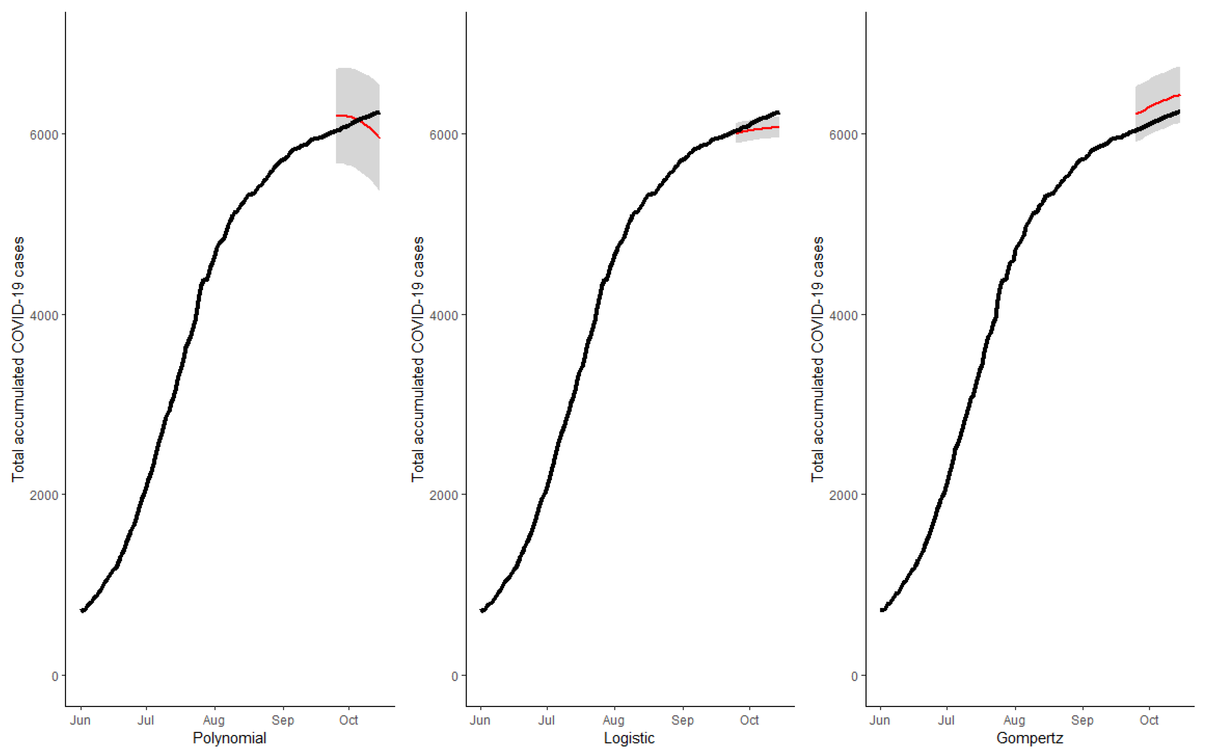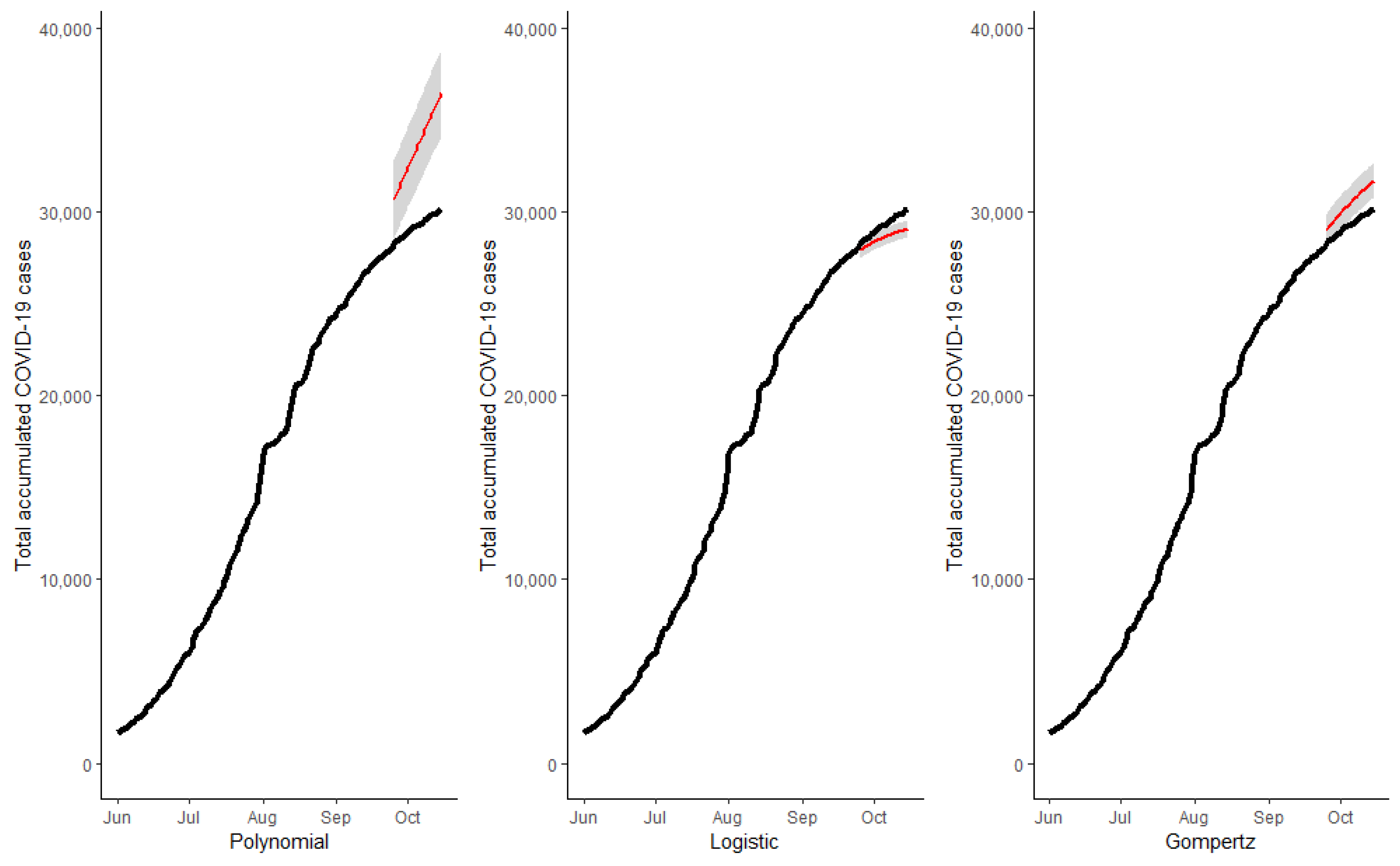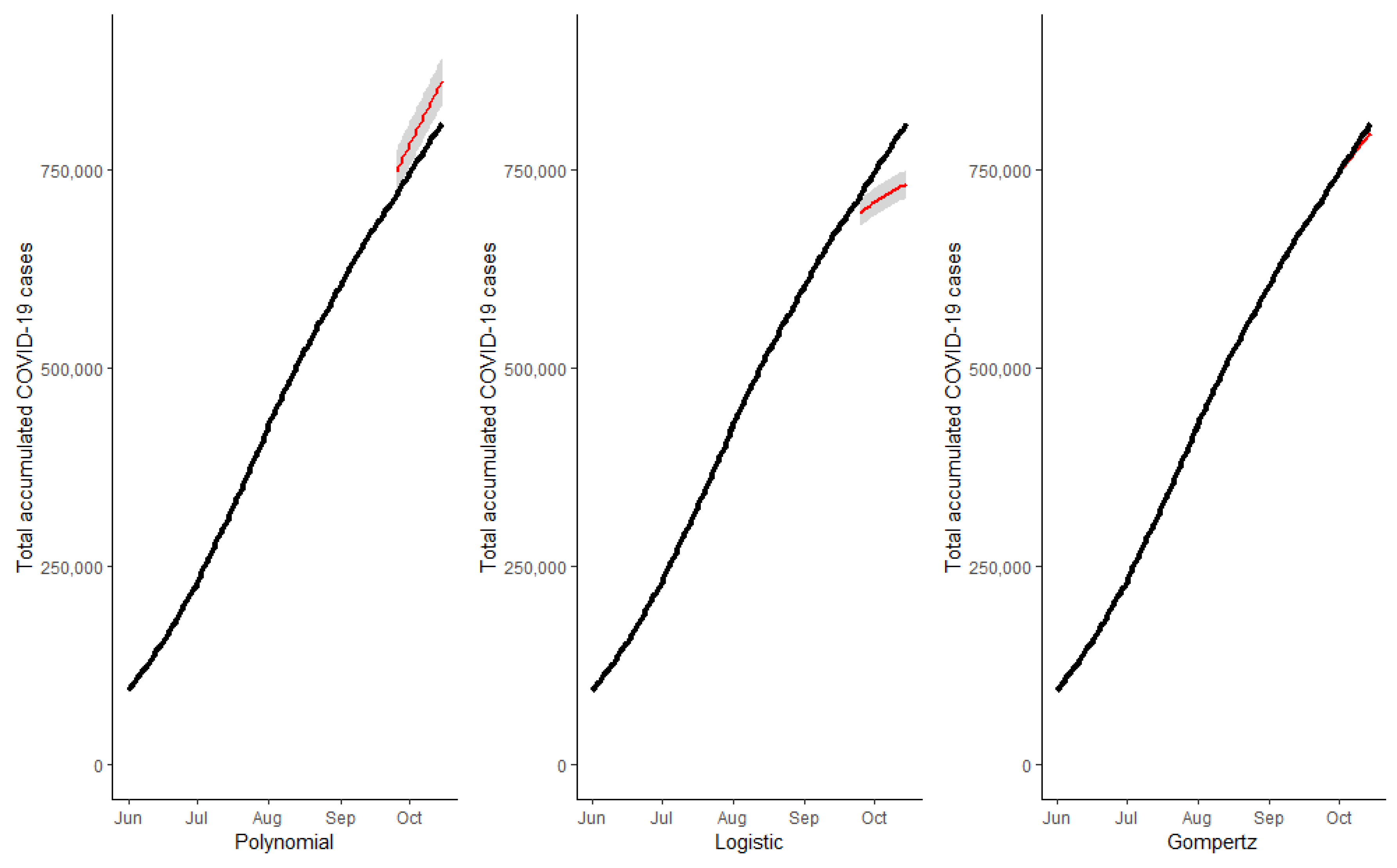Figure 4, Figure 5, Figure 6 and Figure 7 show the cumulative total cases of COVID-19 through 15 October (21 days out of the initial sample which was 24 September) for the four case studies (solid black line). These figures also show, with a red line, the point predictions made by each of the three models, as well as the area covered by the prediction intervals of said estimates with gray shading. In Figure 4, we can observe that the predictions made by the logistic and Gompertz models were relatively good, but not so in the case of the polynomial model, which even predicted a decrease in the total accumulated cases (which was not possible in the context studied). Figure 5 corresponds to the state of Tamaulipas—in this figure, we can see that the worst predictions were also made by the polynomial model. In Figure 6, we can see the predictions for the state of Quintana Roo, wherein the model that best made predictions was the logistic one, and the total number of cases was overestimated by the two other models. Regarding the predictions made for the country, in Figure 7, we can see that the best predictions, by far, were made by the Gompertz model.

Table 4. Root mean square error (RMSE) values for the four case studies for three different models examined.

Date	Models	Mexico	Campeche	Quintana Roo	Tamaulipas
24 September	Polynomial	631.68	17.68	27.29	120.98
	Logistic	608.40	13.15	24.76	113.62
	Gompertz	593.07	14.75	26.70	118.01
20 days after the peak day	Polynomial	557.91	15.13	27.21	127.13
	Logistic	577.16	13.81	25.19	121.63
	Gompertz	556.36	14.37	26.25	123.51
Peak day	Polynomial	495.67	11.00	21.93	88.45
	Logistic	498.42	10.87	22.44	81.66
	Gompertz	482.74	10.92	22.45	85.92
10 days before peak day	Polynomial	427.87	8.07	16.01	50.46
	Logistic	436.88	7.77	16.20	50.73
	Gompertz	406.15	8.02	16.26	50.20
20 days before peak day	Polynomial	386.63	6.33	13.79	42.74
	Logistic	392.59	6.27	13.46	41.11
	Gompertz	374.12	6.25	13.60	42.39
30 days before peak day	Polynomial	326.50	5.72	11.45	30.72
	Logistic	325.06	5.43	11.55	30.21
	Gompertz	303.46	5.51	11.37	30.48

Smaller values of RMSE value being lower indicate better fit.

shows the root mean square error (RMSE) of each model proposed for the three state case studies and at the national level at the six time periods of interest.

As a result of the 21-day predictions mentioned above, the number of new cases of COVID-19 can be obtained, and the results for the four case studies and the three models are shown in

Table 5. Daily new COVID-19 cases predicted from total cumulative cases in Mexico.

			Polynomial		Logistic		Gompertz
Date	Cases	New Cases	% Prediction Error	New Cases	Accumulated	New Cases	Accumulated	New Cases
9/24/20	715,457		3.40%		3.60%		−0.11%
9/25/20	720,858	5401	3.48%	6001	−3.72%	2502	−0.16%	4285
9/26/20	726,431	5573	3.50%	5938	−4.16%	2407	−0.35%	4227
9/27/20	730,317	3886	3.74%	5924	−4.37%	2336	−0.30%	4182
9/28/20	733,717	3400	4.04%	5910	−4.51%	2267	−0.20%	4137
9/29/20	738,163	4446	4.19%	5896	−4.82%	2200	−0.25%	4092
9/30/20	743,216	5053	4.27%	5881	−5.22%	2134	−0.38%	4047
10/1/20	748,315	5099	4.34%	5866	−5.63%	2070	−0.53%	4003
10/2/20	753,090	4775	4.44%	5850	−6.00%	2007	−0.63%	3958
10/3/20	757,953	4863	4.53%	5833	−6.40%	1946	−0.76%	3914
10/4/20	761,665	3712	4.76%	5816	−6.63%	1886	−0.73%	3870
10/5/20	765,082	3417	5.02%	5798	−6.84%	1828	−0.67%	3826
10/6/20	769,558	4476	5.15%	5780	−7.20%	1772	−0.76%	3782
10/7/20	774,020	4462	5.27%	5762	−7.56%	1716	−0.85%	3739
10/8/20	779,127	5107	5.31%	5742	−8.02%	1663	−1.03%	3696
10/9/20	784,580	5453	5.31%	5723	−8.54%	1610	−1.26%	3652
10/10/20	789,779	5199	5.33%	5702	−9.02%	1559	−1.46%	3610
10/11/20	792,920	3141	5.60%	5682	−9.23%	1510	−1.40%	3567
10/12/20	796,399	3479	5.82%	5660	−9.49%	1462	−1.38%	3524
10/13/20	800,474	4075	5.96%	5639	−9.83%	1415	−1.45%	3482
10/14/20	805,512	5038	5.99%	5616	−10.32%	1369	−1.65%	3440
10/15/20	810,883	5371	5.98%	5593	−10.85%	1325	−1.89%	3399

,

Table 6. Daily new COVID-19 cases predicted from total cumulative cases in the state of Campeche.

			Polynomial		Logistic		Gompertz
Date	Cases	New Cases	Accumulated	New Cases	Accumulated	New Cases	Accumulated	New Cases
9/24/20	6027		2.64%		−0.40%		2.90%
9/25/20	6033	6	2.57%	5	−0.48%	5	2.92%	15
9/26/20	6046	13	2.41%	3	−0.60%	5	2.93%	14
9/27/20	6056	10	2.27%	1	−0.68%	5	2.99%	14
9/28/20	6072	16	2.01%	0	−0.87%	5	2.95%	14
9/29/20	6076	4	1.92%	−2 *	−0.86%	5	3.09%	13
9/30/20	6089	13	1.66%	−3 *	−1.00%	4	3.08%	13
10/1/20	6106	17	1.31%	−5 *	−1.21%	4	3.00%	13
10/2/20	6116	10	1.05%	−6 *	−1.31%	4	3.03%	12
10/3/20	6128	12	0.73%	−8 *	−1.45%	4	3.02%	12
10/4/20	6143	15	0.33%	−10 *	−1.64%	4	2.96%	11
10/5/20	6155	12	−0.04%	−11 *	−1.78%	3	2.94%	11
10/6/20	6165	10	−0.41%	−13 *	−1.89%	3	2.95%	11
10/7/20	6173	8	−0.78%	−15 *	−1.97%	3	2.99%	11
10/8/20	6182	9	−1.20%	−16 *	−2.07%	3	3.00%	10
10/9/20	6191	9	−1.64%	−18 *	−2.17%	3	3.01%	10
10/10/20	6194	3	−2.02%	−20 *	−2.18%	3	3.11%	10
10/11/20	6209	15	−2.63%	−21 *	−2.39%	2	3.02%	9
10/12/20	6224	15	−3.28%	−23 *	−2.59%	2	2.92%	9
10/13/20	6230	6	−3.81%	−25 *	−2.66%	2	2.96%	9
10/14/20	6237	7	−4.39%	−27 *	−2.74%	2	2.98%	9
10/15/20	6246	9	−5.05%	−29 *	−2.85%	2	2.97%	8

* Due to the nature of the polynomial model that was used only for Stage I, we predicted a decrease in the total number of cases accumulated that did not match reality, as we can see from the negative numbers. The table above reflects the disadvantage of this type of model.

,

Table 7. Daily new COVID-19 cases predicted from total cumulative cases in the state of Quintana Roo.

			Polynomial		Logistic		Gompertz
Date	Cases	New Cases	Accumulated	New Cases	Accumulated	New Cases	Accumulated	New Cases
9/24/20	11,455		5.13%		0.30%		3.80%
9/25/20	11,500	45	5.03%	77	0.02%	39	3.96%	66
9/26/20	11,583	83	4.93%	75	−0.41%	34	3.79%	65
9/27/20	11,621	38	5.19%	74	−0.46%	32	3.99%	65
9/28/20	11,653	32	5.49%	73	−0.46%	31	4.23%	64
9/29/20	11,693	40	5.72%	72	−0.54%	31	4.40%	63
9/30/20	11,742	49	5.87%	72	−0.71%	30	4.49%	63
10/1/20	11,832	90	5.68%	71	−1.23%	29	4.24%	62
10/2/20	11,888	56	5.76%	70	−1.47%	28	4.26%	61
10/3/20	11,956	68	5.74%	69	−1.82%	27	4.18%	61
10/4/20	12,013	57	5.79%	68	−2.08%	26	4.18%	60
10/5/20	12,048	35	6.01%	67	−2.16%	25	4.36%	59
10/6/20	12,055	7	6.44%	66	−2.01%	24	4.74%	58
10/7/20	12,146	91	6.21%	65	−2.57%	24	4.46%	58
10/8/20	12,172	26	6.48%	65	−2.59%	23	4.68%	57
10/9/20	12,179	7	6.88%	64	−2.46%	22	5.05%	56
10/10/20	12,189	10	7.25%	63	−2.36%	21	5.38%	56
10/11/20	12,241	52	7.29%	62	−2.62%	21	5.38%	55
10/12/20	12,347	106	6.91%	61	−3.34%	20	4.96%	54
10/13/20	12,366	19	7.19%	60	−3.33%	19	5.21%	54
10/14/20	12,405	39	7.30%	59	−3.50%	19	5.30%	53
10/15/20	12,447	42	7.39%	58	−3.69%	18	5.35%	52

and

Table 8. Daily new COVID-19 cases predicted from total cumulative cases in the state of Tamaulipas.

			Polynomial		Logistic		Gompertz
Date	Cases	New Cases	Accumulated	New Cases	Accumulated	New Cases	Accumulated	New Cases
9/24/20	28,159		7.60%		−1.20%		2.30%
9/25/20	28,320	161	7.85%	295	−1.30%	85	2.35%	165
9/26/20	28,454	134	8.29%	294	−1.48%	82	2.44%	162
9/27/20	28,534	80	8.90%	294	−1.48%	79	2.69%	159
9/28/20	28,606	72	9.52%	294	−1.46%	76	2.96%	156
9/29/20	28,764	158	9.86%	293	−1.76%	73	2.93%	153
9/30/20	28,847	83	10.42%	293	−1.80%	70	3.14%	151
10/1/20	28,946	99	10.92%	293	−1.91%	67	3.29%	148
10/2/20	29,085	139	11.29%	292	−2.17%	64	3.29%	145
10/3/20	29,224	139	11.65%	292	−2.44%	61	3.29%	143
10/4/20	29,266	42	12.30%	292	−2.37%	59	3.60%	140
10/5/20	29,319	53	12.90%	291	−2.36%	56	3.86%	138
10/6/20	29,364	45	13.51%	291	−2.32%	54	4.14%	135
10/7/20	29,496	132	13.86%	290	−2.60%	52	4.12%	133
10/8/20	29,617	121	14.23%	289	−2.84%	49	4.13%	130
10/9/20	29,719	102	14.65%	289	−3.03%	47	4.20%	128
10/10/20	29,813	94	15.08%	288	−3.19%	45	4.28%	125
10/11/20	29,873	60	15.60%	288	−3.24%	43	4.47%	123
10/12/20	29,877	4	16.27%	287	−3.11%	41	4.82%	121
10/13/20	30,073	196	16.39%	286	−3.64%	40	4.56%	118
10/14/20	30,104	31	16.97%	286	−3.62%	38	4.81%	116
10/15/20	30,224	120	17.28%	285	−3.90%	36	4.78%	114

. These results are based on the official data source of the daily releases issued by the Mexican Secretaria de Salud on its website https://coronavirus.gob.mx/as of 15 October 2020 [5].

4.2. Autocorrelation

An autoregressive model was fitted to the residuals of the logistics and Gompertz models estimated in a single stage to eliminate the autocorrelation. We fit an autoregressive model to the logistic and Gompertz functions to eliminate the residual autocorrelation. The analysis revealed that the inclusion of an autoregressive component of the second order improved the fit of the data. For example, for the state of Aguascalientes, Figure 8a,b shows the autocorrelation residual and partial autocorrelation plots for models without the autoregressive terms. In these figures, it is clear that the residuals show a pattern of dependency. Furthermore, Figure 8c,d demonstrates a good fit, and there is no evidence of linear relationship. The patterns in the data revealed that nonlinear models with autoregressive terms met assumptions of independence. The models showed good fit while accounting for autocorrelation of residuals while providing better interpretability of the model coefficients in terms of growth rate, maximum number of cases, and initial number of cases. Thus, the model proposed in this paper produces a substantial improvement of the predictions.

5. Conclusions

The modeling of the COVID-19 cases is a unique challenge for statisticians, considering the fact that the data are limited and there are often delays in updating the data. Our approach to modeling the pandemic can provide assistance to decision-making officials for containing and anticipating a “second wave” of the COVID-19 pandemic in Mexico. We divided the pandemic data into two stages, and at each stage, three two-step models were adjusted. In Stage I, as can be seen in Table 3, the polynomial model of order three with an autoregressive error component of order one was computed through applying the Prais–Winsten or Cochrane–Orcutt estimation, which had a better performance than nonlinear growth models. In Stage II, after the peak of COVID-19 cases, two-step nonlinear growth models outperformed the polynomial model. Further, the models used in this paper were different than those used in predictive models using time series or machine learning; however, our model met the assumption of independence of residuals, and the interpretability of our model was superior to those of machine learning—particularly for government officials without a statistics or machine learning background.

Although it is not the objective of this research, another purpose for the proposed models concerns the identification of the peak of the pandemic. That is, an analytical way to know if the pandemic is currently in a period of growth, peak, or decline of sustained cases is through the adjustments of the models. For example, at the moment that any of the non-linear growth models fits significantly better than the other models, we will be at the point of sustained reduction of daily cases, which would mean that the peak has already passed, and that said model must be used to make predictions of total cases and obtain insights of the pandemic at that point.

In summary, this paper showed the efficacy of utilizing two different types of models estimated in two stages (stages depending on the state of the pandemic). The majority of the efforts to model the COVID-19 pandemic are nonlinear models, such as logistic and Gompertz [4,5]. However, these models do not take into account autoregression, thus possibly skewing short-, medium-, and long-term predictions. In contrast with the SIR models, where it is necessary to fix or assume a few initial parameters, our proposed models do not require initial parameter assumptions. Our first recommendation, due to simplicity in fitting the model, is that in the early stages of the pandemic where there was an exponential growth (during or before the peak), one should utilize a polynomial model of the third order estimated with an autoregressive component. Our second recommendation is that for the later, more advanced stages when the peak of the pandemic was reached, one should utilize a nonlinear growth model (logistic or Gompertz) estimated with an autoregressive component. In the event that two models show the best fit, if any of these is the polynomial model, it will be necessary to question whether it is in the public health decisionmakers’ interest to have insights (provided by the βs of the non-linear growth models) of the current state of the pandemic; if yes, then we recommend using the non-linear growth model. In the opposite case, where it is not in the interest of the decisionmakers to know insights of the pandemic, the use of the polynomial model is recommended since it does not require initial values for its estimation. Another scenario could be that within the tie, there are two linear growth models, wherein either of the two can be used.

This research is not without limitations. The projections resulting from the models were estimated without considering any type of intervention. In other words, the intervention effects—such as mask mandates, lockdowns, social distancing, or vaccines—are not considered in our models. Any of the aforementioned variables should be considered with care. Regarding vaccination, as this article was being written, there was no official site of the Mexican government where the total number of people vaccinated could be retrieved, only unofficial sites where progress is reported; however, these numbers are not trustworthy. Regarding the measures of lockdowns and use of face masks, given the federal nature of the country, the states of the republic are free to take or not take actions on their population; thus, to analyze any variable of this nature, an exhaustive study must be carried out on the states that took similar measures, and the effect of these measures must be evaluated by means of an effect or additive or multiplicative variable in the statistical model.

Due to the characteristics of the models used, the atypical characteristics of the COVID-19 pandemic, and the results and information derived from the monitoring strategy—well known in epidemiology science as SENTINEL Prevention Model—the following should be considered:

The data show a lot of variability from one day to another. Part of the noise caused by the dynamics of new case records was smoothed out by pre-processing the data (moving average) and the AR (1) component of the model; in future work, to further reduce the noise, we could add complex structures in the residuals, such as ARMA, ARIMA, or SARIMA. Furthermore, at the time of the data cut-off date, the second wave of the pandemic had not yet occurred. In the event that it is required to use this model for a second wave of the pandemic, care must be taken with the estimation of the components of the non-linear models (specifically the autoregressive and nonlinear component). That is, the nonlinear models used are not designed to model spikes in cases (second wave or third waves), and this will affect the estimation of parameters—such as growth speed, maximum cases, and the autoregressive component—being able to obtain estimates out of context of the pandemic (very high or low numbers), or uniroot problems in the time series component.

As previously mentioned, the residual autocorrelation analysis was performed, looking for linear autocorrelations. Regarding the precision of the predictions, future research will focus on comparing our proposed models against machine learning and artificial intelligence models. In some cases, such as the state of Aguascalientes, it was necessary to add a second order autoregressive component.

The benefit of utilizing a second-order autoregressive component is shown in

Table 9. Comparison models by goodness of fit criteria for the state of Aguascalientes.

Model Type	Durbin–Watson	AIC	BIC
Gompertz	(3, 139) = 0.0569	1509.95	1519.08
Gompertz + AR (1)	(4, 139) = 1.1040	968.83	980.56
Gompertz + AR (1) + AR (2)	(5, 139) = 2.2986 *	937.6	952.27

* p-value > 0.05 taken from Durbin–Watson statistical table values.

for the state of Aguascalientes (before 20 August 2020). For the Gompertz nonlinear growth model, we corrected for the dependency between observations by including an autocorrelation term of the second order in the model that considerably improved the overall fit criteria. Thus, we recommend the inclusion of an autoregressive term of the second order when modeling COVID-19 case growth.

References

1. Villela, D.A. Discrete time forecasting of epidemics. Infect. Dis. Model. 2020, 5, 189–196. [Google Scholar] [CrossRef] [PubMed]
2. Ribeiro, M.H.D.M.; da Silva, R.G.; Mariani, V.C.; dos Santos Coelho, L. Short-term forecasting COVID-19 cumulative confirmed cases: Perspectives for Brazil. Chaos Solitons Fractals 2020, 135, 109853. [Google Scholar] [CrossRef] [PubMed]
3. De Pinho, S.Z.; de Carvalho, L.R.; Mischan, M.M.; Passos, J.R.d.S. Critical points on growth curves in autoregressive and mixed models. Sci. Agric. 2014, 71, 30–37. [Google Scholar] [CrossRef] [Green Version]
4. Montgomery, D.C.; Peck, E.A.; Vining, G.G. Introduction to Linear Regression Analysis; John Wiley & Sons: Hoboken, NJ, USA, 2021. [Google Scholar]
5. Gobierno de Mexico, Secretaria de Salud. Datos Abiertos Dirección General de Epidemiología. Available online: https://www.gob.mx/salud/documentos/datos-abiertos-152127 (accessed on 18 August 2021).
6. Zhang, X.; Ma, R.; Wang, L. Predicting turning point, duration and attack rate of COVID-19 outbreaks in major Western countries. Chaos Solitons Fractals 2020, 135, 109829. [Google Scholar] [CrossRef] [PubMed]
7. Mazurek, J.; Nenickova, Z. Predicting the Number of Total COVID-19 Cases and Deaths in the USA by the Gompertz Curve; Elsevier: Amsterdam, The Netherlands, 2020; submitted. [Google Scholar]
8. Batista, M. Estimation of the final size of the COVID-19 epidemic. medRxiv 2020. [Google Scholar] [CrossRef] [Green Version]
9. Box, G.E.; Jenkins, G.M.; Reinsel, G.C.; Ljung, G.M. Time Series Analysis, Control, and Forecasting; John Wiley & Sons: Hoboken, NJ, USA, 2015. [Google Scholar]
10. Lin, Q.; Zhao, S.; Gao, D.; Lou, Y.; Yang, S.; Musa, S.S.; Wang, M.H.; Cai, Y.; Wang, W.; Yang, L.; et al. A conceptual model for the coronavirus disease 2019 (COVID-19) outbreak in Wuhan, China with individual reaction and governmental action. Int. J. Infect. Dis. 2020, 93, 211–216. [Google Scholar] [CrossRef]
11. World Health Organization. WHO Coronavirus (COVID-19) Dashboard. 2020. Available online: https://covid19.who.int (accessed on 18 August 2021).
12. Murphy, K.M.; Topel, R.H. Estimation and Inference in Two-Step Econometric Models. J. Bus. Econ. Stat. 1985, 3, 370–379. [Google Scholar]
13. Oxford. Cochrane—Orcuttprocedure. Available online: https://www.oxfordreference.com/view/10.1093/oi/authority.20110803095620898 (accessed on 18 August 2021).
14. Calafiore, G.C.; Novara, C.; Possieri, C. A time-varying SIRD model for the COVID-19 contagion in Italy. Annu. Rev. Control 2020, 50, 361–372. [Google Scholar] [CrossRef]
15. Carli, R.; Cavone, G.; Epicoco, N.; Scarabaggio, P.; Dotoli, M. Model predictive control to mitigate the COVID-19 outbreak in a multi-region scenario. Annu. Rev. Control 2020, 50, 373–393. [Google Scholar] [CrossRef]
16. Coutin Marie, G. Utilización de modelos ARIMA para la vigilancia de enfermedades transmisibles. Rev. Cuba. Salud Pública 2007, 33. [Google Scholar]
17. Benvenuto, D.; Giovanetti, M.; Vassallo, L.; Angeletti, S.; Ciccozzi, M. Application of the ARIMA model on the COVID-2019 epidemic dataset. Data Brief 2020, 29, 105340. [Google Scholar] [CrossRef] [PubMed]
18. Chakraborty, T.; Ghosh, I. Real-time forecasts and risk assessment of novel coronavirus (COVID-19) cases: A data-driven analysis. Chaos Solitons Fractals 2020, 135, 109850. [Google Scholar] [CrossRef] [PubMed]
19. Grzegorczyk, A. Application of the Richards function to the description of leaf area growth in maize (Zea mays L.). Acta Soc. Bot. Pol. 1994, 63, 5–7. [Google Scholar] [CrossRef]
20. Roosa, K.; Lee, Y.; Luo, R.; Kirpich, A.; Rothenberg, R.; Hyman, J.; Yan, P.; Chowell, G. Real-time forecasts of the COVID-19 epidemic in China from February 5th to February 24th, 2020. Infect. Dis. Model. 2020, 5, 256–263. [Google Scholar] [CrossRef] [PubMed]
21. Shen, C.Y. Logistic growth modelling of COVID-19 proliferation in China and its international implications. Int. J. Infect. Dis. 2020, 96, 582–589. [Google Scholar] [CrossRef]
22. Chimmula, V.K.R.; Zhang, L. Time series forecasting of COVID-19 transmission in Canada using LSTM networks. Chaos Solitons Fractals 2020, 135, 109864. [Google Scholar] [CrossRef]
23. Menon, V.K. Prediction of number of cases expected and estimation of the final size of coronavirus epidemic in India using the logistic model and genetic algorithm. arXiv 2020, arXiv:2003.12017. preprint. [Google Scholar]
24. Choi, S.; Jung, E.; Choi, B.Y.; Hur, Y.J.; Ki, M. High reproduction number of Middle East respiratory syndrome coronavirus in nosocomial outbreaks: Mathematical modelling in Saudi Arabia and South Korea. J. Hosp. Infect. 2018, 99, 162–168. [Google Scholar] [CrossRef] [Green Version]
25. Porter, T.; Kebreab, E.; Kuhi, H.D.; Lopez, S.; Strathe, A.B.; France, J. Flexible alternatives to the Gompertz equation for describing growth with age in turkey hens. Poult. Sci. 2010, 89, 371–378. [Google Scholar] [CrossRef]
26. Tariq, M.M.; Iqbal, F.; Eyduran, E.; Bajwa, M.A.; Huma, Z.E.; Waheed, A. Comparison of non-linear functions to describe the growth in Mengali sheep breed of Balochistan. Pak. J. Zool. 2013, 45, 661–665. [Google Scholar]
27. Vuong, Q.H. Likelihood ratio tests for model selection and non-nested hypotheses. Econom. J. Econom. Soc. 1989, 57, 307–333. [Google Scholar] [CrossRef] [Green Version]
28. Zhou, J.; Tse, G.; Lee, S.; Liu, T.; Wu, W.K.; Zeng, D.; Wong, I.C.K.; Zhang, Q.; Cheung, B.M.Y. Identifying main and interaction effects of risk factors to predict intensive care admission in patients hospitalized with COVID-19: A retrospective cohort study in Hong Kong. medRxiv 2020. [Google Scholar] [CrossRef]
29. R Core Team. R: A Language and Environment for Statistical Computing (Version 3.0. 2); R Foundation for Statistical Computing: Vienna, Austria, 2019. [Google Scholar]
30. Statacorp. Stata Statistical Software: Release 15; StataCorp LP: College Station, TX, USA, 2017. [Google Scholar]
Figure 1. (a) Accumulated cases and (b) new daily cases of COVID-19 in Mexico.
Mathematics 09 02180 g001
Figure 2. Graphical abstract of the methodology.
Mathematics 09 02180 g002
Figure 3. Polynomial versus a nonlinear growth model.
Mathematics 09 02180 g003
Figure 4. Forecast for total accumulated cases at 21 days for the state of Campeche.
Mathematics 09 02180 g004
Figure 5. Forecast for total accumulated cases at 21 days for the state of Tamaulipas.
Mathematics 09 02180 g005
Figure 6. Forecast for total accumulated cases at 21 days for the state of Quintana Roo.
Mathematics 09 02180 g006
Figure 7. Forecast for total accumulated cases at 21 days at the national level in Mexico.
Mathematics 09 02180 g007
Figure 8. Analysis of autocorrelation in residuals.
Mathematics 09 02180 g008