Convergence Analysis of a Numerical Method for a Fractional Model of Fluid Flow in Fractured Porous Media

Abstract

The present paper is devoted to the construction and study of numerical methods for solving an initial boundary value problem for a differential equation containing several terms with fractional time derivatives in the sense of Caputo. This equation is suitable for describing the process of fluid flow in fractured porous media under some physical assumptions, and has an important applied significance in petroleum engineering. Two different approaches to constructing numerical schemes depending on orders of the fractional derivatives are proposed. The semi-discrete and fully discrete numerical schemes for solving the problem are analyzed. The construction of a fully discrete scheme is based on applying the finite difference approximation to time derivatives and the finite element method in the spatial direction. The approximation of the fractional derivatives in the sense of Caputo is carried out using the L1-method. The convergence of both numerical schemes is rigorously proved. The results of numerical tests conducted for model problems are provided to confirm the theoretical analysis. In addition, the proposed computational method is applied to study the flow of oil in a fractured porous medium within the framework of the considered model. Based on the results of the numerical tests, it was concluded that the model reproduces the characteristic features of the fluid flow process in the medium under consideration.

1. Introduction

Comprehensive study of the fluid flow phenomenon in fractured porous media has received considerable attention due to its practical significance in variety of industrial processes, particularly in petroleum engineering. This is due to the fact that a significant percentage of world’s oil reserves are concentrated in these complex formations, and therefore accurate representation of the flow behavior in the reservoir is relevant due to involvement of these deposits in production.

In recent decades, several conceptual approaches to modeling flows in fractured media have been proposed, an extensive overview of which is presented in [1,2]. The fundamental conceptual models include single- and multi-continuum models, discrete fracture matrix and discrete fracture network models. The works of many authors (e.g., [3,4,5]) are aimed at a qualitative comparison of these models.

Some authors [6,7,8] are of the opinion that the fluid motion in a fractured medium cannot be adequately described within the framework of classical theory of fluid flow in porous media, assuming that the nature of the flow depends not only on the current state of the process but also on the previous history of changes in this process. This phenomenon is known as memory in petroleum engineering. Caputo [9] introduced a memory formalism using the apparatus of fractional calculus and proposed the time fractional modification of the classical Darcy’s law. This idea was further developed by many authors (e.g., [6,7,10,11,12,13,14]), and a number of fractional differential generalizations of the classical model have been developed that take into account the memory and spatial correlations effects in porous media (see a literature review in [15]). In this case, the order of the fractional derivative determines the degree of memory impact on patterns of the flow. The experimental studies [16,17] show that fractional differential equations can be effectively used to obtain a more realistic description of fluid flow in porous media.

There are several definitions of the fractional derivative and fractional integral in fractional calculus, an overview of which can be found in [18,19]. In the development of mathematical models of fluid flow in porous media under different physical assumptions, various authors have used fractional time derivatives in the sense of Caputo [7,8,9,20,21], Riemann–Liouville [6,22], Caputo–Fabrizio [23,24], Atangana–Baleanu [25] and others [26] to account for memory effects, whereas the Riemann–Liouville derivative is mainly used to describe nonlocality in the spatial direction [6,27]. In the study of dynamic processes in fractured fractal media, a fractional temporal derivative in the sense of Caputo has an advantage, since it is given by the convolution of the power law kernel and the derivative of the function. In the case of using the Riemann–Liouville time derivatives, difficulties arise in determining and physical treatment of initial conditions [28]. Despite the obvious, from a computational aspect, advantages of the recently developed Caputo–Fabrizio derivative associated with the non-singularity of the kernel, some authors doubt the correctness of its application to account for memory effects [29].

Despite the existence of studies devoted to obtaining an analytical solution of some fractional differential equations (see, e.g., [30,31]), it is a quite challenging problem in the general case. A large number of papers are devoted to the construction and study of numerical methods for solving fractional differential equations which include finite difference methods [32,33,34,35,36,37,38], finite element methods [39,40,41,42], finite volume methods [43,44], collocation methods [45], and many others. In addition, the construction of computational schemes is also based on using a certain formula for discretizing the fractional derivatives included in the equation. There are several approximations of the fractional derivative in the sense of Caputo, e.g., the L1-method [32,46,47,48], modified L1-method [49], backward Euler method [50] with convergence order $\left(2-\nu \right)$; L1-2 formula [51] and L2-1${}_{\sigma }$ scheme [38] with convergence order $\left(3-\nu \right)$; L1-3 scheme [52] with convergence order $\left(4-\nu \right)$, and many others [53], where $\nu$ is the fractional derivative order.

In [6], a new model of fluid flow in a fractured porous medium is derived. The proposed model is based on utilizing the fractional differential analogue of the fluid motion law describing fluid flow in natural fractured porous media in which the fractures are distributed uniformly on average over the volume. The model is also constructed under the assumption that porosity and density are functions not only of pressure but also its fractional time derivatives. However, the paper does not pay attention to the numerical implementation of the mathematical model. Furthermore, the literature review did not reveal any papers devoted to the numerical implementation or obtaining an analytical solution to this model.

In this paper, we conduct for the first time a numerical analysis of the mathematical model of fluid flow in a fractured porous medium proposed in [6] with some reasonable simplifying assumptions. The governing equation of the model contains several terms with fractional derivatives of various orders $\alpha ,\beta \in \left(0,2\right)$, $\gamma \in \left(0,1\right)$, as well as a term with the derivative of a function of some expression that contains both time fractional and integer spatial derivatives. Unlike [6], we use the Caputo fractional derivative which does not lack a physical interpretation of the initial conditions.

We consider three special cases of the fractional differential equation and propose two different implicit finite difference/finite element approaches to constructing a numerical scheme for solving the problem depending on orders of the fractional derivatives. The first approach, applied to the case $\alpha ,\beta ,\gamma \in \left(0,1\right)$, is based on the use of a higher order approximation to the integer temporal derivative. The second numerical scheme, applied to the cases $\alpha \in \left(1,2\right)$, $\beta ,\gamma \in \left(0,1\right)$ and $\beta \in \left(1,2\right)$, $\alpha ,\gamma \in \left(0,1\right)$, uses a different approach and is based on utilizing of a Crank–Nicolson type scheme.

We rigorously prove the convergence of both semi-discrete and fully discrete schemes for both constructed numerical methods. The theoretical convergence order of both computational schemes is confirmed by the results of numerous computational experiments.

Further, we consider a slightly more realistic example, which is aimed at studying the flow of oil in a fractured porous medium, and present the results of computational experiments depending on orders of the fractional derivatives. In addition, the results of the numerical implementation of the classical model of fluid flow in a porous medium are presented for comparison. Based on the results of the numerical tests, it was concluded that the model reproduces the characteristic features of the process of fluid flow in a fractured porous medium.

The paper starts by providing a brief derivation of the model equation and defining the problem formulation in Section 2.1. In Section 2.2, semi-discrete formulations of the problem are determined and convergence theorems are proved. The construction of fully discrete schemes and the proof of two convergence theorems is given in Section 2.3. Section 3 describes the experimental study and presents the results of several numerical tests conducted to verify the theoretical analysis, while Section 4 provides the discussion of the obtained results.

2. Materials and Methods

2.1. Formulation of the Problem

In the classical theory of fluid flow in porous media, the governing equations of the single-phase isothermal flow of a viscous fluid through an isotropic porous medium include the continuity equation and Darcy’s law:

$${\partial }_t\left(\varphi \rho \right)+\nabla ·\left(\rho \overrightarrow{U}\right)=f,$$

(1)

$$\overrightarrow{U}=-\frac{k}{\tilde{\mu }}\nabla p,$$

(2)

where $\varphi$ and k are the porosity and absolute permeability of the medium; p, $\rho$, and $\tilde{\mu }$ are the pressure, density, and viscosity of the fluid, respectively; $\overrightarrow{U}$ is the velocity vector; f is the density of mass sources. For simplicity, the influence of gravitational forces is neglected.

One approach to describe fluid flow through a fractured porous medium is to replace the above medium with some model homogeneous porous medium with power-law memory. Due to the fact that porosity depends on the pressure of the fluid and on the stress-strain state of a medium exhibiting viscoelastic properties, it is concluded in [6] that porosity is a function not only of pressure but also of its fractional derivative or fractional integral:

$$\varphi =\varphi \left(p,{\partial }_{0,t}^{\overline{\alpha }}p\right),\overline{\alpha }\in \left(-1,1\right),$$

(3)

where ${\partial }_{0,t}^{\overline{\alpha }}$ refers to the Caputo fractional differentiation operator which for positive real numbers $\nu$ such that $n-1<\nu <n$, $n=1,2,3,\dots$ is defined as [18]

$${\partial }_{0,t}^{\nu }p\left(t\right)=\frac{1}{\Gamma \left(n-\nu \right)}{\int }_0^t\frac{p^{\left(n\right)}\left(\theta \right)}{{\left(t-\theta \right)}^{1+\nu -n}}d\theta .$$

(4)

The negative order Caputo fractional differentiation operator ${\partial }_{0,t}^{-\nu }$ is equivalent to the Caputo fractional integration operator, $I_{0,t}^{\nu }$, which can be defined as [54,55]

$${\partial }_{0,t}^{-\nu }p\left(t\right)\equiv I_{0,t}^{\nu }p\left(t\right)=g\left(t\right)+\frac{1}{\Gamma \left(\nu \right)}{\int }_0^{t}p\left(\theta \right){\left(t-\theta \right)}^{\nu -1}d\theta ,t>0,0<\nu \le 1,$$

where $g\left(t\right)$ is a function defined in [54]. In addition, we use the following fractional differential generalization of the classical state equation [56]:

$$\rho =\rho \left(p,{\partial }_{0,t}^{\overline{\beta }}p\right),\overline{\beta }\in \left(-1,1\right).$$

(5)

To account for the effect of fractures on the fluid flow process, we use the following generalized motion law which describes fluid flow in natural fractured porous media in which the fractures are distributed uniformly on average over the volume [6]:

$$\overrightarrow{U}=-\mathcal{F}\left({\partial }_{0,t}^{\gamma }\left(\nabla p\right)\right)\frac{\nabla p}{\left|\nabla p\right|},\gamma \in \left(0,1\right),$$

(6)

where $\mathcal{F}\left(z\right)$ is a given function. Substituting (3)–(6) into (1), we obtain the following nonlinear fractional differential equation describing the flow of a viscoelastic fluid in a fractured porous medium:

$$\varphi \left(c_{f1}+c_{\varphi 1}\right){\partial }_{t}p+\varphi c_{\varphi \overline{\alpha }}{\partial }_{0,t}^{\overline{\alpha }+1}p+\varphi c_{f\overline{\beta }}{\partial }_{0,t}^{\overline{\beta }+1}p-\nabla ·\left(\mathcal{F}\left({\partial }_{0,t}^{\gamma }\left(\nabla p\right)\right)\frac{\nabla p}{\left|\nabla p\right|}\right)$$

$$-\mathcal{F}\left({\partial }_{0,t}^{\gamma }\left(\nabla p\right)\right)\frac{\nabla p}{\left|\nabla p\right|}\left(c_{f1}\nabla p+c_{f\overline{\beta }}{\partial }_{0,t}^{\overline{\beta }}\left(\nabla p\right)\right)={\overline{f}}_0,$$

(7)

where ${\displaystyle {\overline{f}}_0=\frac{f}{\rho }}$; ${\displaystyle c_{f1}=\frac{1}{\rho }\frac{\partial \rho }{\partial p}}$ and ${\displaystyle c_{\varphi 1}=\frac{1}{\varphi }\frac{\partial \varphi }{\partial p}}$ are classical isothermal compressibility of a fluid and a porous medium, respectively, and ${\displaystyle c_{f\overline{\beta }}=\frac{1}{\rho }\frac{\partial \rho }{\partial \left({\partial }_{0,t}^{\overline{\beta }}p\right)}}$, ${\displaystyle c_{\varphi \overline{\alpha }}=\frac{1}{\varphi }\frac{\partial \varphi }{\partial \left({\partial }_{0,t}^{\overline{\alpha }}p\right)}}$ are their generalized fractional differential counterparts [6].

A complete analysis of the resulting Equation (7) is quite difficult due to the presence of a large number of parameters. Let us introduce some simplifying assumptions that are not overly restrictive in practical applications. First, we assume that the flow is one-dimensional. Following [6], we neglect the last term in the left-hand side of (7) due to its smallness compared to the fourth term. Furthermore, the porosity function $\varphi$ is assumed to be linear with respect to its arguments:

$$\varphi =b_{1}p+b_2{\partial }_{0,t}^{\overline{\alpha }}p,$$

where $b_1,b_2$ are some positive constants. Let us further assume that the fluid density explicitly depends only on the fractional derivative of the pressure, and there exists a positive constant quantity $b_3$ such that $\varphi c_{f\overline{\beta }}=b_3$. Taking into account the above assumptions, (7) reduces to the following form:

$${\partial }_{t}p+{\overline{c}}_{\varphi \alpha }{\partial }_{0,t}^{\overline{\alpha }+1}p+{\overline{c}}_{f\beta }{\partial }_{0,t}^{\overline{\beta }+1}p-{\left(\mathcal{F}\left({\partial }_{0,t}^{\gamma }{p}_x\right)\right)}_x={\overline{f}}_0,$$

(8)

where ${\overline{c}}_{\varphi \alpha }=b_2/b_1$, ${\overline{c}}_{f\beta }=b_3/b_1$ are positive constants.

For ease of presentation, we introduce the notation $\alpha =\overline{\alpha }+1$, $\beta =\overline{\beta }+1$ and restrict ourselves to considering the following three cases:

$$\begin{array}{cccc}\mathbf{Case}\mathbf{I}.\hfill & \overline{\alpha }\in \left(-1,0\right),\hfill & \overline{\beta }\in \left(-1,0\right),\hfill & \gamma \in \left(0,1\right),\hfill \\ \mathbf{Case}\mathbf{II}.\hfill & \overline{\alpha }\in \left(0,1\right),\hfill & \overline{\beta }=\overline{\alpha }-1\in \left(-1,0\right),\hfill & \gamma \in \left(0,1\right),\hfill \\ \mathbf{Case}\mathbf{III}.\hfill & \overline{\beta }\in \left(0,1\right),\hfill & \overline{\alpha }=\overline{\beta }-1\in \left(-1,0\right),\hfill & \gamma \in \left(0,1\right).\hfill \end{array}$$

Thus, in this paper, we consider the following problem in ${\overline{Q}}_T=\overline{\Omega }\times \left[0,T\right]$, where $\Omega =\left(0,1\right)$.

Problem 1.

Find p such that

$$\left\{\begin{array}{cc}{\partial }_{t}p+{\overline{c}}_{\varphi \alpha }{\partial }_{0,t}^{\alpha }p+{\overline{c}}_{f\beta }{\partial }_{0,t}^{\beta }p-{\left(\mathcal{F}\left({\partial }_{0,t}^{\gamma }{p}_x\right)\right)}_x={\overline{f}}_0,\hfill & \left(x,t\right)\in \Omega \times \left(0,T\right],\hfill \\ p\left(x,0\right)=p_0\left(x\right),\hfill & x\in \overline{\Omega },\hfill \\ p\left(0,t\right)=p\left(1,t\right)=0,\hfill & t\in \left(0,T\right],\hfill \end{array}\right.$$

when $\alpha ,\beta ,\gamma \in \left(0,1\right)$;

$$\left\{\begin{array}{cc}{\partial }_{t}p+{\overline{c}}_{\varphi \alpha }{\partial }_{0,t}^{\overline{\alpha }+1}p+{\overline{c}}_{f\beta }{\partial }_{0,t}^{\overline{\alpha }}p-{\left(\mathcal{F}\left({\partial }_{0,t}^{\gamma }{p}_x\right)\right)}_x={\overline{f}}_0,\hfill & \left(x,t\right)\in \Omega \times \left(0,T\right],\hfill \\ p\left(x,0\right)=p_0\left(x\right),{\partial }_{t}p\left(x,0\right)=u_0\left(x\right),\hfill & x\in \overline{\Omega },\hfill \\ p\left(0,t\right)=p\left(1,t\right)=0,\hfill & t\in \left(0,T\right],\hfill \end{array}\right.$$

when $\overline{\alpha },\gamma \in \left(0,1\right)$;

$$\left\{\begin{array}{cc}{\partial }_{t}p+{\overline{c}}_{\varphi \alpha }{\partial }_{0,t}^{\overline{\beta }}p+{\overline{c}}_{f\beta }{\partial }_{0,t}^{\overline{\beta }+1}p-{\left(\mathcal{F}\left({\partial }_{0,t}^{\gamma }{p}_x\right)\right)}_x={\overline{f}}_0,\hfill & \left(x,t\right)\in \Omega \times \left(0,T\right],\hfill \\ p\left(x,0\right)=p_0\left(x\right),{\partial }_{t}p\left(x,0\right)=u_0\left(x\right),\hfill & x\in \overline{\Omega },\hfill \\ p\left(0,t\right)=p\left(1,t\right)=0,\hfill & t\in \left(0,T\right],\hfill \end{array}\right.$$

when $\overline{\beta },\gamma \in \left(0,1\right)$.

The following additional assumptions will be used throughout the paper:

Assumption 1.

Problem 1 has a unique solution having sufficient number of derivatives required to perform the analysis.

Assumption 2.

In Case I, $\mathcal{F}$ is of the form

$$\mathcal{F}\left(\phi \right)=\mu \phi +\chi \left(x,t\right),$$

where χ is a given function, $\mu >0$ is a constant. In Cases II and III, $\mathcal{F}$ is of the form

$$\mathcal{F}\left(\phi \right)=\mu \left({\partial }_t\phi +\phi \right).$$

Assumption 3.

In Cases II and III, we assume that ${\overline{c}}_{\varphi \alpha }={\overline{c}}_{f\beta }$.

We adopt the standard notations of spaces $L^q\left(\Omega \right)$ and Sobolev spaces $W^{k,q}\left(\Omega \right)$ with the special case $q=2$ denoted by $H^k\left(\Omega \right)$ [57]. In addition, $\left(·,·\right)$ denotes the scalar product in $L^2\left(\Omega \right)$ and ${∥·∥}_k$ denotes the norm in $H^k\left(\Omega \right)$.

Now we define the variational formulation of Problem 1. Since the sought solution belongs to different functional spaces depending on orders of the fractional derivatives, $\overline{\alpha }$, $\overline{\beta }$ and $\overline{\gamma }$, let us consider the variational formulations of Problem 1 separately in accordance with Cases I, II, and III.

Problem 2.

Find $p\in H^1\left(0,T;H_0^1\left(\Omega \right)\right)$ such that for all $v\in H_0^1\left(\Omega \right)$:

$$\left({\partial }_{t}p,v\right)+{\overline{c}}_{\varphi \alpha }\left({\partial }_{0,t}^{\alpha }p,v\right)+{\overline{c}}_{f\beta }\left({\partial }_{0,t}^{\beta }p,v\right)+\left(\mathcal{F}\left({\partial }_{0,t}^{\gamma }{p}_x\right),v_x\right)=\left({\overline{f}}_0,v\right),$$

(9)

$$p\left(x,0\right)=p_0\left(x\right),x\in \overline{\Omega },$$

(10)

where $\alpha ,\beta ,\gamma \in \left(0,1\right)$.

Problem 3.

Find $p\in H^{1+q}\left(0,T;H_0^1\left(\Omega \right)\right)$, $q=max\left\{\overline{\alpha },\gamma \right\}$ such that for all $v\in H_0^1\left(\Omega \right)$:

$$\left({\partial }_{t}p,v\right)+{\overline{c}}_{\varphi \alpha }\left({\partial }_{0,t}^{\overline{\alpha }}\left({\partial }_{t}p+p\right),v\right)+\mu \left({\partial }_{0,t}^{\gamma }\left({\partial }_t{p}_x+p_x\right),v_x\right)=\left({\overline{f}}_0,v\right),$$

(11)

$$p\left(x,0\right)=p_0\left(x\right),{\partial }_{t}p\left(x,0\right)=u_0\left(x\right),x\in \overline{\Omega },$$

(12)

where $\overline{\alpha },\gamma \in \left(0,1\right)$.

Problem 4.

Find $p\in H^{1+q}\left(0,T;H_0^1\left(\Omega \right)\right)$, $q=max\left\{\overline{\beta },\gamma \right\}$ such that for all $v\in H_0^1\left(\Omega \right)$:

$$\left({\partial }_{t}p,v\right)+{\overline{c}}_{f\beta }\left({\partial }_{0,t}^{\overline{\beta }}\left({\partial }_{t}p+p\right),v\right)+\mu \left({\partial }_{0,t}^{\gamma }\left({\partial }_t{p}_x+p_x\right),v_x\right)=\left({\overline{f}}_0,v\right),$$

(13)

$$p\left(x,0\right)=p_0\left(x\right),{\partial }_{t}p\left(x,0\right)=u_0\left(x\right),x\in \overline{\Omega },$$

(14)

where $\overline{\beta },\gamma \in \left(0,1\right)$.

2.2. Semi-Discrete Schemes

2.2.1. Construction of the Semi-Discrete Schemes

To define a semi-discrete formulation of Problem 1 with respect to time, it is necessary to approximate both integer and fractional derivatives in time. To this end, we introduce a uniform partition of the time interval $\left[0,T\right]$ by points $t_n=n\tau$, $\tau >0$, $n=0,1,\dots ,N$ such that $N\tau =T$. Let $p^n$ denote a semi-discrete approximation of the function p at $t=t_n$. Additionally, we sometimes use the notation $p(·,t)=p\left(t\right)$ for brevity.

We use the following approximation formula for the fractional derivative in the sense of Caputo.

Lemma 1.

The discrete analog ${\Delta }_{0,t}^{\nu }{p}^n$ of the fractional derivative in the sense of Caputo ${\partial }_{0,t}^{\nu }p\left(t_n\right)$ of order $0<\nu <1$ can be represented as [32]

$${\Delta }_{0,t}^{\nu }{p}^n=\sum _{s=1}^n{\delta }_{n,s}^{\nu }\left(p^s-p^{s-1}\right),$$

(15)

where

$${\delta }_{n,s}^{\nu }=\frac{{\tau }^{-\nu }}{\Gamma \left(2-\nu \right)}\left[{\left(n-s+1\right)}^{1-\nu }-{\left(n-s\right)}^{1-\nu }\right].$$

Moreover, the following estimate holds for $r_n^{\nu }={\partial }_{0,t}^{\nu }p\left(t_n\right)-{\Delta }_{0,t}^{\nu }{p}^n$:

$$\left|r_n^{\nu }\right|\le \frac{5-\nu }{8\left(1-\nu \right)}\underset{0\le t\le t_n}{max}\left|{\partial }_t^{2}p\left(t\right)\right|{\tau }^{2-\nu }.$$

Some obvious properties of the coefficients ${\delta }_{n,s}^{\nu }$ presented in Lemma 1 are as below.

Lemma 2.

The following properties hold for the coefficients ${\delta }_{n,s}^{\nu }$, $s=1,2,\dots ,n$:

(a) ${\delta }_{n,s}^{\nu }>0$, $s=1,2,\dots ,n$;

(b) ${\delta }_{n,s}^{\nu }<{\delta }_{n,s+1}^{\nu }$, $s=1,2,\dots ,n-1$;

(c) ${\delta }_{n,s}^{\nu }={\delta }_{n-1,s-1}^{\nu }$;

(d) ${\displaystyle \sum _{s=1}^n{\delta }_{n,s}^{\nu }=\frac{n{t}_n^{-\nu }}{\Gamma \left(2-\nu \right)}}$.

In this paper, we propose two different approaches to constructing numerical schemes depending on the orders of the fractional derivatives. The first approach is applied to Case I and is based on the use of the fractional derivative approximation (15) and a higher order approximation of the integer temporal derivative which is defined as

$${\partial }_{t}p\left(t_n\right)=\left\{\begin{array}{cc}{\displaystyle \frac{3p^n-4p^{n-1}+p^{n-2}}{2\tau }+\frac{{\tau }^2}{3}{\partial }_t^3\left({\zeta }_n\right),}\hfill & n\ge 2,{\zeta }_n\in \left(t_{n-2},t_n\right),\hfill \\ {\displaystyle \frac{p^1-p^0}{\tau }+\frac{\tau }{2}{\partial }_t^{2}p\left({\zeta }_1\right),}\hfill & n=1,{\zeta }_1\in \left(t_0,t_1\right).\hfill \end{array}\right.$$

(16)

Let us define a semi-discrete formulation of Problem 1 corresponding to Case I as follows.

Problem 5.

Let ${\left\{p^i\right\}}_{i=0}^{n-1}$, $p^i\in H_0^1\left(\Omega \right)$ be given where $p^0=p_0\left(x\right)$, $x\in \overline{\Omega }$ and $n\ge 1$. Find $p^n\in H_0^1\left(\Omega \right)$ satisfying the following identities for all $v\in H_0^1\left(\Omega \right)$ and $\alpha ,\beta ,\gamma \in \left(0,1\right)$:

$$\left(\frac{p^1-p^0}{\tau },v\right)+{\overline{c}}_{\varphi \alpha }\left({\Delta }_{0,t}^{\alpha }{p}^1,v\right)+{\overline{c}}_{f\beta }\left({\Delta }_{0,t}^{\beta }{p}^1,v\right)+\left(\mathcal{F}\left({\Delta }_{0,t}^{\gamma }{p}_x^1\right),v_x\right)=\left({\overline{f}}_0^1,v\right),n=1,$$

(17)

$$\left(\frac{3p^n-4p^{n-1}+p^{n-2}}{2\tau },v\right)+{\overline{c}}_{\varphi \alpha }\left({\Delta }_{0,t}^{\alpha }{p}^n,v\right)+{\overline{c}}_{f\beta }\left({\Delta }_{0,t}^{\beta }{p}^n,v\right)$$

$$+\left(\mathcal{F}\left({\Delta }_{0,t}^{\gamma }{p}_x^n\right),v_x\right)=\left({\overline{f}}_0^n,v\right),n\ge 2.$$

(18)

The second proposed numerical scheme is applied to Cases II and III and is based on the use of the fractional derivative approximation (15) and the Crank–Nicolson type scheme. To this end, introduce the notations

$$p^{n-1/2}=\frac{1}{2}\left(p^n+p^{n-1}\right),{\Delta }_t{p}^{n-1/2}=\frac{1}{\tau }\left(p^n-p^{n-1}\right).$$

(19)

Then the semi-discrete formulations corresponding to Cases II and III is stated as follows.

Problem 6.

Let ${\left\{p^i\right\}}_{i=0}^{n-1}$, $p^i\in H_0^1\left(\Omega \right)$ be given such that $p^0=p_0\left(x\right)$ and ${\Delta }_t{p}^{1/2}=u_0\left(x\right)$, $x\in \overline{\Omega }$. Find $p^n\in H_0^1\left(\Omega \right)$, $n\ge 2$ satisfying the following identity for all $v\in H_0^1\left(\Omega \right)$ and $\overline{\alpha },\gamma \in \left(0,1\right)$:

$$\left({\Delta }_t{p}^{n-1/2},v\right)+{\overline{c}}_{\varphi \alpha }\left({\Delta }_{0,t}^{\overline{\alpha }}\left({\Delta }_t{p}^{n-1/2}+p^{n-1/2}\right),v\right)$$

$$+\mu \left({\Delta }_{0,t}^{\gamma }\left({\Delta }_t{p}_x^{n-1/2}+p_x^{n-1/2}\right),v_x\right)=\left({\overline{f}}_0^{n-1/2},v\right).$$

(20)

Problem 7.

Let ${\left\{p^i\right\}}_{i=0}^{n-1}$, $p^i\in H_0^1\left(\Omega \right)$ be given such that $p^0=p_0\left(x\right)$ and ${\Delta }_t{p}^{1/2}=u_0\left(x\right)$, $x\in \overline{\Omega }$. Find $p^n\in H_0^1\left(\Omega \right)$, $n\ge 2$ satisfying the following identity for all $v\in H_0^1\left(\Omega \right)$ and $\overline{\beta },\gamma \in \left(0,1\right)$:

$$\left({\Delta }_t{p}^{n-1/2},v\right)+{\overline{c}}_{f\beta }\left({\Delta }_{0,t}^{\overline{\beta }}\left({\Delta }_t{p}^{n-1/2}+p^{n-1/2}\right),v\right)$$

$$+\mu \left({\Delta }_{0,t}^{\gamma }\left({\Delta }_t{p}_x^{n-1/2}+p_x^{n-1/2}\right),v_x\right)=\left({\overline{f}}_0^{n-1/2},v\right).$$

(21)

2.2.2. Error Estimates of the Semi-Discrete Schemes

First, we prove a few auxiliary lemmas. Lemmas 3 and 4 below are used to obtain estimates of terms containing fractional and integer time derivatives.

Lemma 3.

The following inequality holds for ${\Delta }_{0,t}^{\nu }{p}^n$, $0<\nu <1$, $n\ge 1$:

$$\left({\Delta }_{0,t}^{\nu }{p}^n,p^n\right)\ge {\Theta }_n^{\nu }-{\Theta }_{n-1}^{\nu }-\frac{1}{2}{\delta }_{n,1}^{\nu }{∥p^0∥}_0^2,$$

where ${\displaystyle {\Theta }_i^{\nu }=\frac{1}{2}\left({\delta }_{i,1}^{\nu }{∥p^1∥}_0^2+{\delta }_{i,2}^{\nu }{∥p^2∥}_0^2+\cdots +{\delta }_{i,i}^{\nu }{∥p^i∥}_0^2\right)}$, $i\ge 1$ and ${\Theta }_0^{\nu }=0$.

Proof. 

It follows from Lemma 1 that

$$\left({\Delta }_{0,t}^{\nu }{p}^n,p^n\right)={\delta }_{n,n}^{\nu }{∥p^n∥}_0^2-\sum _{s=1}^{n-1}\left({\delta }_{n,s+1}^{\nu }-{\delta }_{n,s}^{\nu }\right)\left(p^s,p^n\right)-{\delta }_{n,1}^{\nu }\left(p^0,p^n\right).$$

Using the Cauchy–Schwarz inequality and Lemma 2 taking into account the elementary inequality $ab\le \frac{1}{2}\left(a^2+b^2\right)$, we obtain

$$\begin{array}{cc}\hfill \left({\Delta }_{0,t}^{\nu }{p}^n,p^n\right)& \ge {\delta }_{n,n}^{\nu }{∥p^n∥}_0^2-\sum _{s=1}^{n-1}\left({\delta }_{n,s+1}^{\nu }-{\delta }_{n,s}^{\nu }\right){∥p^s∥}_0{∥p^n∥}_0-{\delta }_{n,1}^{\nu }{∥p^0∥}_0{∥p^n∥}_0\hfill \\ & \ge \frac{1}{2}\sum _{s=1}^n{\delta }_{n,s}^{\nu }{∥p^s∥}_0^2-\frac{1}{2}\sum _{s=1}^{n-1}{\delta }_{n,s+1}^{\nu }{∥p^s∥}_0^2-\frac{1}{2}{\delta }_{n,1}^{\nu }{∥p^0∥}_0^2\hfill \\ & ={\Theta }_n^{\nu }-{\Theta }_{n-1}^{\nu }-\frac{1}{2}{\delta }_{n,1}^{\nu }{∥p^0∥}_0^2.\hfill \end{array}$$

The lemma is proved. □

Lemma 4.

Let the sequence ${\left\{p^i\right\}}_{i=0}^n$, $p^i\in L^2\left(\Omega \right)$ be given. Then

$$\left(\frac{p^n-p^{n-1}}{\tau },p^n\right)=\frac{1}{2\tau }\left({∥p^n∥}_0^2-{∥p^{n-1}∥}_0^2+{∥p^n-p^{n-1}∥}_0^2\right),n\ge 1,$$

$$\left(\frac{3p^n-4p^{n-1}+p^{n-2}}{2\tau },p^n\right)=\frac{1}{4\tau }\left({∥p^n∥}_0^2+{∥2p^n-p^{n-1}∥}_0^2-{∥p^{n-1}∥}_0^2\right.$$

$$\left.-{∥2p^{n-1}-p^{n-2}∥}_0^2+{∥p^n-2p^{n-1}+p^{n-2}∥}_0^2\right),n\ge 2.$$

Proof. 

This lemma can be verified directly. □

In addition, we formulate the discrete analogue of Gronwall’s lemma which will be used several times throughout the paper.

Lemma 5

([58]). If $\left\{a_n\right\}$ and $\left\{b_n\right\}$ are two positive sequences, $\left\{c_n\right\}$ is a monotone positive sequence, and they satisfy the inequalities $a_0+b_0\le c_0$, ${\displaystyle a_n+b_n\le c_n+\lambda \sum _{i=0}^{n-1}{a}_i}$, $\lambda >0$, then the following estimate holds:

$$a_n+b_n\le c_{n}exp\left(n\lambda \right),n=0,1,2,\dots$$

Now we prove the main results of the section. The symbol C below denotes a positive constant that does not depend on $\tau$ and may take different values.

Theorem 1.

Let ${\left\{p^i\right\}}_{i=0}^N$, $p^i\in H_0^1\left(\Omega \right)$ be the solution of Problem 5 and p be the solution of Problem 1. Then the following inequality holds for $p^n\in H_0^1\left(\Omega \right)$ under Assumptions 1 and 2:

$${∥p\left(t_n\right)-p^n∥}_0+\tau \sqrt{\frac{2c_0}{T}}{∥p\left(t_n\right)-p^n∥}_1\le C\left({\tau }^{2-\alpha }+{\tau }^{2-\beta }+{\tau }^{2-\gamma }\right),$$

where $\alpha ,\beta ,\gamma \in \left(0,1\right)$ and ${\displaystyle c_0=min\left\{{\overline{c}}_{\varphi \alpha }{\delta }_{n,1}^{\alpha },{\overline{c}}_{f\beta }{\delta }_{n,1}^{\beta },\mu {\delta }_{n,1}^{\gamma }\right\}}$.

Proof. 

Denote ${\pi }^n=p\left(t_n\right)-p^n$. By substracting (17) and (18) from (9) at $t=t_n$, taking $v={\pi }^n$, using (16) and Lemma 4, we obtain:

$${∥{\pi }^1∥}_0^2-{∥{\pi }^0∥}_0^2+{∥{\pi }^1-{\pi }^0∥}_0^2+2\tau {\overline{c}}_{\varphi \alpha }\left({\partial }_{0,t}^{\alpha }p\left(t_1\right)-{\Delta }_{0,t}^{\alpha }{p}^1,{\pi }^1\right)$$

$$+2\tau {\overline{c}}_{f\beta }\left({\partial }_{0,t}^{\beta }p\left(t_1\right)-{\Delta }_{0,t}^{\beta }{p}^1,{\pi }^1\right)$$

$$+2\tau \left(\mathcal{F}\left({\partial }_{0,t}^{\gamma }{p}_x\left(t_1\right)\right)-\mathcal{F}\left({\Delta }_{0,t}^{\gamma }{p}_x^1\right),{\pi }_x^1\right)+{\tau }^2\left({\partial }_t^{2}p\left({\zeta }_1\right),{\pi }^1\right)=0,$$

(22)

$${∥{\pi }^n∥}_0^2+{∥2{\pi }^n-{\pi }^{n-1}∥}_0^2-{∥{\pi }^{n-1}∥}_0^2-{∥2{\pi }^{n-1}-{\pi }^{n-2}∥}_0^2+{∥{\pi }^n-2{\pi }^{n-1}+{\pi }^{n-2}∥}_0^2$$

$$+4\tau {\overline{c}}_{\varphi \alpha }\left({\partial }_{0,t}^{\alpha }p\left(t_n\right)-{\Delta }_{0,t}^{\alpha }{p}^n,{\pi }^n\right)+4\tau {\overline{c}}_{f\beta }\left({\partial }_{0,t}^{\beta }p\left(t_n\right)-{\Delta }_{0,t}^{\beta }{p}^n,{\pi }^n\right)$$

$$+4\tau \left(\mathcal{F}\left({\partial }_{0,t}^{\gamma }{p}_x\left(t_n\right)\right)-\mathcal{F}\left({\Delta }_{0,t}^{\gamma }{p}_x^n\right),{\pi }_x^n\right)+\frac{4{\tau }^3}{3}\left({\partial }_t^{3}p\left({\zeta }_n\right),{\pi }^n\right)=0,n\ge 2.$$

(23)

By using Assumption 2 and Lemma 3, we have:

$$\begin{array}{cc}\hfill \left({\partial }_{0,t}^{\alpha }p\left(t_n\right)-{\Delta }_{0,t}^{\alpha }{p}^n,{\pi }^n\right)& =\left(r_n^{\alpha },{\pi }^n\right)+\left({\Delta }_{0,t}^{\alpha }{\pi }^n,{\pi }^n\right)\hfill \\ & \ge \left(r_n^{\alpha },{\pi }^n\right)+\left({\Theta }_n^{\alpha }-{\Theta }_{n-1}^{\alpha }\right)-\frac{1}{2}{\delta }_{n,1}^{\alpha }{∥{\pi }^0∥}_0^2,\hfill \end{array}$$

(24)

$$\left({\partial }_{0,t}^{\beta }p\left(t_n\right)-{\Delta }_{0,t}^{\beta }{p}^n,{\pi }^n\right)\ge \left(r_n^{\beta },{\pi }^n\right)+\left({\Theta }_n^{\beta }-{\Theta }_{n-1}^{\beta }\right)-\frac{1}{2}{\delta }_{n,1}^{\beta }{∥{\pi }^0∥}_0^2,$$

(25)

$$\begin{array}{cc}\hfill \left(\mathcal{F}\left({\partial }_{0,t}^{\gamma }{p}_x\left(t_n\right)\right)-\mathcal{F}\left({\Delta }_{0,t}^{\gamma }{p}_x^n\right),{\pi }_x^n\right)& =\mu \left({\partial }_{0,t}^{\gamma }{p}_x\left(t_n\right)-{\Delta }_{0,t}^{\gamma }{p}_x^n,{\pi }_x^n\right)\hfill \\ & \ge \mu \left(r_n^{\gamma },{\pi }_x^n\right)+\mu \left({\Theta }_n^{\gamma }-{\Theta }_{n-1}^{\gamma }\right)-\frac{1}{2}\mu {\delta }_{n,1}^{\gamma }{∥{\pi }_x^0∥}_0^2,\hfill \end{array}$$

(26)

where

$$\begin{array}{ccc}{\displaystyle {\Theta }_n^{\overline{\nu }}=\frac{1}{2}\sum _{s=1}^n{\delta }_{n,s}^{\overline{\nu }}{∥{\pi }^s∥}_0^2},\hfill & & r_n^{\overline{\nu }}={\partial }_{0,t}^{\overline{\nu }}p\left(t_n\right)-{\Delta }_{0,t}^{\overline{\nu }}p\left(t_n\right),\overline{\nu }\in \left\{\alpha ,\beta \right\},\hfill \\ {\displaystyle {\Theta }_n^{\gamma }=\frac{1}{2}\sum _{s=1}^n{\delta }_{n,s}^{\gamma }{∥{\pi }_x^s∥}_0^2},\hfill & & r_n^{\gamma }={\partial }_{0,t}^{\gamma }{p}_x\left(t_n\right)-{\Delta }_{0,t}^{\gamma }{p}_x\left(t_n\right)\hfill \end{array}$$

(27)

and $r_n^{\nu }=O\left({\tau }^{2-\nu }\right)$, $\nu \in \left\{\alpha ,\beta ,\gamma \right\}$ by Lemma 1.

Taking into account inequalities (24)–(26), we obtain from (22) and (23) that

$${∥{\pi }^1∥}_0^2+2\tau {\Theta }_1\le {\tau }^2{∥{\partial }_t^{2}p\left({\zeta }_1\right)∥}_0{∥{\pi }^1∥}_0+2\tau {\overline{c}}_{\varphi \alpha }{∥r_1^{\alpha }∥}_0{∥{\pi }^1∥}_0$$

$$+2\tau {\overline{c}}_{f\beta }{∥r_1^{\beta }∥}_0{∥{\pi }^1∥}_0+2\tau \mu {∥r_1^{\gamma }∥}_0{∥{\pi }_x^1∥}_0,$$

(28)

$${∥{\pi }^n∥}_0^2+{∥2{\pi }^n-{\pi }^{n-1}∥}_0^2+4\tau {\Theta }_n+{∥{\pi }^n-2{\pi }^{n-1}+{\pi }^{n-2}∥}_0^2$$

$$\le {∥{\pi }^{n-1}∥}_0^2+{∥2{\pi }^{n-1}-{\pi }^{n-2}∥}_0^2+4\tau {\Theta }_{n-1}+\frac{4{\tau }^3}{3}{∥{\partial }_t^{3}p\left({\zeta }_n\right)∥}_0{∥{\pi }^n∥}_0$$

$$+4\tau {\overline{c}}_{\varphi \alpha }{∥r_n^{\alpha }∥}_0{∥{\pi }^n∥}_0+4\tau {\overline{c}}_{f\beta }{∥r_n^{\beta }∥}_0{∥{\pi }^n∥}_0+4\tau \mu {∥r_n^{\gamma }∥}_0{∥{\pi }_x^n∥}_0,n\ge 2$$

(29)

where

$${\Theta }_n={\overline{c}}_{\varphi \alpha }{\Theta }_n^{\alpha }+{\overline{c}}_{f\beta }{\Theta }_n^{\beta }+\mu {\Theta }_n^{\gamma }.$$

(30)

Sum (29) with respect to n from 2 to n, make use of Young inequality to get

$${∥{\pi }^n∥}_0^2+{∥2{\pi }^n-{\pi }^{n-1}∥}_0^2+4\tau {\Theta }_n\le {∥{\pi }^1∥}_0^2+{∥2{\pi }^1-{\pi }^0∥}_0^2+4\tau {\Theta }_1$$

$$+\frac{\tau }{2}\left(\left({\overline{c}}_{\varphi \alpha }{\delta }_{n,n}^{\alpha }+{\overline{c}}_{f\beta }{\delta }_{n,n}^{\beta }\right){∥{\pi }^n∥}_0^2+\mu {\delta }_{n,n}^{\gamma }{∥{\pi }_x^n∥}_0^2\right)$$

$$+\frac{{\tau }^2}{2}\sum _{i=2}^{n-1}\left(\left({\overline{c}}_{\varphi \alpha }{\delta }_{n,n}^{\alpha }+{\overline{c}}_{f\beta }{\delta }_{n,n}^{\beta }\right){∥{\pi }^i∥}_0^2+\mu {\delta }_{n,n}^{\gamma }{∥{\pi }_x^i∥}_0^2\right)$$

$$+\frac{C\tau }{{\delta }_{n,n}^{\sigma }}{\left({\tau }^2{∥{\partial }_t^{3}p\left({\zeta }_n\right)∥}_{L^{\infty }\left(t_{n-1},t_n;L^2\left(\Omega \right)\right)}+{∥r_n^{\alpha }∥}_0+{∥r_n^{\beta }∥}_0\right)}^2+\frac{C\tau }{{\delta }_{n,n}^{\gamma }}{∥r_n^{\gamma }∥}_0^2$$

$$+\frac{C}{{\delta }_{n,n}^{\sigma }}\sum _{i=2}^{n-1}{\left({\tau }^2{∥{\partial }_t^{3}p\left({\zeta }_i\right)∥}_{L^{\infty }\left(0,t_{n-1};L^2\left(\Omega \right)\right)}+{∥r_i^{\alpha }∥}_0+{∥r_i^{\beta }∥}_0\right)}^2+\frac{C}{{\delta }_{n,n}^{\gamma }}\sum _{i=2}^n{∥r_i^{\gamma }∥}_0^2,$$

where $\sigma =min\left\{\alpha ,\beta \right\}$. Using Lemma 1 as well as the facts that

$$\frac{1}{2}\left({\overline{c}}_{\varphi \alpha }{\delta }_{i,i}^{\alpha }+{\overline{c}}_{f\beta }{\delta }_{i,i}^{\beta }\right){∥{\pi }^i∥}_0^2+\frac{1}{2}\mu {\delta }_{i,i}^{\gamma }{∥{\pi }_x^i∥}_0^2\le {\Theta }_i$$

(31)

and ${\left({\delta }_{n,n}^{\nu }\right)}^{-1}<\Gamma \left(2-\nu \right)T^{\nu }$, we arrive at

$${∥{\pi }^n∥}_0^2+2\tau {\Theta }_n\le 5{∥{\pi }^1∥}_0^2+4\tau {\Theta }_1+{\tau }^2\sum _{i=2}^{n-1}{\Theta }_i+C{\tau }^{4-2\alpha }+C{\tau }^{4-2\beta }+C{\tau }^{4-2\gamma }.$$

(32)

By applying Lemma 5, we conclude that

$${∥{\pi }^n∥}_0^2+2\tau {\Theta }_n\le C\left({∥{\pi }^1∥}_0^2+\tau {\Theta }_1+{\tau }^{4-2\alpha }+{\tau }^{4-2\beta }+{\tau }^{4-2\gamma }\right).$$

(33)

Estimate the right-hand side of (28) using the Cauchy–Schwarz and Young inequalities and apply Lemma 1 to obtain

$${∥{\pi }^1∥}_0^2+4\tau {\Theta }_1\le \frac{\tau }{2}\left(\left({\overline{c}}_{\varphi \alpha }{\delta }_{1,1}^{\alpha }+{\overline{c}}_{f\beta }{\delta }_{1,1}^{\beta }\right){∥{\pi }^1∥}_0^2+\mu {\delta }_{1,1}^{\gamma }{∥{\pi }_x^1∥}_0^2\right)$$

$$+C\tau \left({\tau }^{4-2\alpha }+{\tau }^{4-2\beta }+{\tau }^{4-2\gamma }\right).$$

Making use of (31), we get

$${∥{\pi }^1∥}_0^2+2\tau {\Theta }_1\le C\tau \left({\tau }^{4-2\alpha }+{\tau }^{4-2\beta }+{\tau }^{4-2\gamma }\right).$$

(34)

Combining (33) and (34), we arrive at the inequality

$${∥{\pi }^n∥}_0^2+2\tau {\Theta }_n\le C\left({\tau }^{4-2\alpha }+{\tau }^{4-2\beta }+{\tau }^{4-2\gamma }\right).$$

Finally, by extracting the square root of both sides of the last inequality and applying the inequality ${\displaystyle {\left(\sum _{i=1}^m{a}_i^2\right)}^{1/2}\ge \frac{1}{\sqrt{m}}\sum _{i=1}^m\left|a_i\right|}$ and noticing that ${\displaystyle \frac{1}{\sqrt{n}}\ge \sqrt{\frac{\tau }{T}}}$, we arrive at the statement of the theorem. □

Before we prove the convergence theorem for Case II, we state the following lemma.

Lemma 6.

The following inequality holds for ${\Delta }_{0,t}^{\nu }{p}^{n-1/2}$, $0<\nu <1$, $n\ge 1$:

$$\left({\Delta }_{0,t}^{\nu }\left({\Delta }_t{p}^{n-1/2}+p^{n-1/2}\right),{\Delta }_t{p}^{n-1/2}+p^{n-1/2}\right)$$

$$\ge {\Theta }_n^{\nu }-{\Theta }_{n-1}^{\nu }-\frac{1}{2}\left({\delta }_{n,2}^{\nu }-{\delta }_{n,1}^{\nu }\right)\left(\frac{1}{\tau }+\frac{1}{2}\right){∥p^1∥}_0^2$$

$$-\frac{1}{2}{\delta }_{n,1}^{\nu }\left(\frac{1}{\tau }+\frac{1}{2}\right){∥p^0∥}_0^2+{\delta }_{n,2}^{\nu }\left(\frac{1}{\tau }-\frac{1}{2}\right)\left(p^0,{\Delta }_t{p}^{n-1/2}+p^{n-1/2}\right),$$

(35)

where ${\displaystyle {\Theta }_i^{\nu }=\frac{1}{2}\sum _{s=2}^i{\delta }_{i,s}^{\nu }{∥{\Delta }_t{p}^{s-1/2}+p^{s-1/2}∥}_0^2}$, $i\ge 1$ and ${\Theta }_0^{\nu }=0$.

Proof. 

The proof of the lemma follows in a similar manner of Lemma 3. □

Theorem 2.

Let ${\left\{p^i\right\}}_{i=0}^N$, $p^i\in H_0^1\left(\Omega \right)$ be the solution of Problem 6 and p be the solution of Problem 1. Then the following inequality holds for $p^n\in H_0^1\left(\Omega \right)$ and $\overline{\alpha },\gamma \in \left(0,1\right)$ under Assumptions 1–3:

$${∥p\left(t_n\right)-p^n∥}_0+\tau \sum _{i=1}^n{∥{\Delta }_t\left(p\left(t_{i-1/2}\right)-p^{i-1/2}\right)∥}_0\le C\left({\tau }^{2-\overline{\alpha }}+{\tau }^{2-\gamma }\right).$$

Proof. 

Denote ${\pi }^n=p\left(t_n\right)-p^n$. Substracting (20) from (11) and taking $v={\Delta }_t{\pi }^{n-1/2}+{\pi }^{n-1/2}$ yields

$$\left({\Delta }_t{\pi }^{n-1/2},{\Delta }_t{\pi }^{n-1/2}+{\pi }^{n-1/2}\right)+{\overline{c}}_{\varphi \alpha }\left({\Delta }_{0,t}^{\overline{\alpha }}\left({\Delta }_t{\pi }^{n-1/2}+{\pi }^{n-1/2}\right),{\Delta }_t{\pi }^{n-1/2}+{\pi }^{n-1/2}\right)$$

$$+\mu \left({\Delta }_{0,t}^{\gamma }\left({\Delta }_t{\pi }_x^{n-1/2}+{\pi }_x^{n-1/2}\right),{\Delta }_t{\pi }_x^{n-1/2}+{\pi }_x^{n-1/2}\right)$$

$$=\left(r_{n-1/2}^{\overline{\alpha }},{\Delta }_t{\pi }^{n-1/2}+{\pi }^{n-1/2}\right)+\left(r_{n-1/2}^{\gamma },{\Delta }_t{\pi }_x^{n-1/2}+{\pi }_x^{n-1/2}\right),$$

(36)

where $\left|r_{n-1/2}^{\overline{\alpha }}\right|\le C{\tau }^{2-\overline{\alpha }}$, $\left|r_{n-1/2}^{\gamma }\right|\le C{\tau }^{2-\gamma }$ easily follows from Lemma 1. Estimate the terms in (36) using Lemma 6:

$$\left({\Delta }_t{\pi }^{n-1/2},{\Delta }_t{\pi }^{n-1/2}+{\pi }^{n-1/2}\right)\ge \frac{1}{2\tau }{∥{\pi }^n∥}_0^2-\frac{1}{2\tau }{∥{\pi }^{n-1}∥}_0^2+{∥{\Delta }_t{\pi }^{n-1/2}∥}_0^2,$$

(37)

$$\left({\Delta }_{0,t}^{\overline{\alpha }}\left({\Delta }_t{\pi }^{n-1/2}+{\pi }^{n-1/2}\right),{\Delta }_t{\pi }^{n-1/2}+{\pi }^{n-1/2}\right)\ge {\Theta }_n^{\overline{\alpha }}-{\Theta }_{n-1}^{\overline{\alpha }},$$

(38)

$$\left({\Delta }_{0,t}^{\gamma }\left({\Delta }_t{\pi }_x^{n-1/2}+{\pi }_x^{n-1/2}\right),{\Delta }_t{\pi }_x^{n-1/2}+{\pi }_x^{n-1/2}\right)\ge {\Theta }_n^{\gamma }-{\Theta }_{n-1}^{\gamma },$$

(39)

$$\left(r_{n-1/2}^{\overline{\alpha }},{\Delta }_t{\pi }^{n-1/2}+{\pi }^{n-1/2}\right)+\left(r_{n-1/2}^{\gamma },{\Delta }_t{\pi }_x^{n-1/2}+{\pi }_x^{n-1/2}\right)\le$$

$$\le C{\tau }^{2-\overline{\alpha }}{∥{\Delta }_t{\pi }^{n-1/2}+{\pi }^{n-1/2}∥}_0+C{\tau }^{2-\gamma }{∥{\Delta }_t{\pi }_x^{n-1/2}+{\pi }_x^{n-1/2}∥}_0,$$

(40)

where

$${\displaystyle {\Theta }_n^{\overline{\alpha }}=\frac{1}{2}\sum _{s=2}^n{\delta }_{n,s}^{\overline{\alpha }}{∥{\Delta }_t{\pi }^{s-1/2}+{\pi }^{s-1/2}∥}_0^2},{\displaystyle {\Theta }_n^{\gamma }=\frac{1}{2}\sum _{s=2}^n{\delta }_{n,s}^{\gamma }{∥{\Delta }_t{\pi }_x^{s-1/2}+{\pi }_x^{s-1/2}∥}_0^2}.$$

Consequently, it follows from (36) that

$${∥{\pi }^n∥}_0^2-{∥{\pi }^{n-1}∥}_0^2+2\tau {∥{\Delta }_t{\pi }^{n-1/2}∥}_0^2+2\tau {\Theta }_n$$

$$\le 2\tau {\Theta }_{n-1}+C{\tau }^{3-\overline{\alpha }}{∥{\Delta }_t{\pi }^{n-1/2}+{\pi }^{n-1/2}∥}_0+C{\tau }^{3-\gamma }{∥{\Delta }_t{\pi }_x^{n-1/2}+{\pi }_x^{n-1/2}∥}_0$$

(41)

where ${\Theta }_n={\overline{c}}_{\varphi \alpha }{\Theta }_n^{\overline{\alpha }}+\mu {\Theta }_n^{\gamma }$. Sum (41) with respect to n from 1 to n to have

$${∥{\pi }^n∥}_0^2+2\tau \sum _{i=1}^n{∥{\Delta }_t{\pi }^{i-1/2}∥}_0^2+2\tau {\Theta }_n\le {∥{\pi }^0∥}_0^2+2\tau {\Theta }_0+C{\tau }^{3-\overline{\alpha }}{∥{\Delta }_t{\pi }^{n-1/2}+{\pi }^{n-1/2}∥}_0$$

$$+C{\tau }^{3-\overline{\alpha }}\sum _{i=1}^{n-1}{∥{\Delta }_t{\pi }^{i-1/2}+{\pi }^{i-1/2}∥}_0+C{\tau }^{3-\gamma }{∥{\Delta }_t{\pi }_x^{n-1/2}+{\pi }_x^{n-1/2}∥}_0$$

$$+C{\tau }^{3-\gamma }\sum _{i=1}^{n-1}{∥{\Delta }_t{\pi }_x^{i-1/2}+{\pi }_x^{i-1/2}∥}_0.$$

Using the same technique as in obtaining the inequality (32) and noticing that

$$\frac{1}{2}{\delta }_{i,s}^{\overline{\alpha }}{∥{\Delta }_t{\pi }^{s-1/2}+{\pi }^{s-1/2}∥}_0^2+\frac{1}{2}{\delta }_{i,s}^{\gamma }{∥{\Delta }_t{\pi }_x^{s-1/2}+{\pi }_x^{s-1/2}∥}_0^2\le {\Theta }_i,$$

we conclude

$${∥{\pi }^n∥}_0^2+2\tau \sum _{i=1}^n{∥{\Delta }_t{\pi }^{i-1/2}∥}_0^2+\tau {\Theta }_n\le {\tau }^2\sum _{i=1}^{n-1}{\Theta }_i+C\left({\tau }^{4-2\overline{\alpha }}+{\tau }^{4-2\gamma }\right).$$

Finally, applying Lemma 5 implies the statement of the theorem. □

Remark 1.

The convergence result of the semi-discrete scheme corresponding to Case III is similar to Theorem 2.

2.3. Fully Discrete Schemes

2.3.1. Construction of the Fully Discrete Schemes

Let ${\mathcal{K}}_h$ denote a uniform partition on $\overline{\Omega }$ with a mesh size h. For $l\in \mathbb{N}$, let $P_l\left(\Omega \right)$ denote the space of polynomials of degree no greater than l on $\Omega$. Define the finite element space as follows:

$$V_h=\left\{v_h\in H_0^1\left(\Omega \right)\cap C^0\left(\overline{\Omega }\right)|{\left.v_h\right|}_e\in P_1\left(e\right),\forall e\in {\mathcal{K}}_h\right\}.$$

Define the projection operator $Q_h:H_0^1\left(\Omega \right)\to V_h$ satisfying

$$\left({\left(Q_{h}p-p\right)}_x,p_{h,x}\right)=0\forall p\in H_0^1\left(\Omega \right),p_h\in V_h.$$

The operator $Q_h$ has the following well known property:

$${∥p-Q_{h}p∥}_0+h{∥p-Q_{h}p∥}_1\le C{h}^2{∥p∥}_2\forall p\in H_0^1\left(\Omega \right)\cap H^2\left(\Omega \right).$$

(42)

Based on the semi-discrete scheme (17), (18) constructed in Section 2.2, we propose the following fully discrete scheme corresponding to Case I.

Problem 8.

Let ${\left\{p_h^i\right\}}_{i=0}^{n-1}$, $p_h^i\in V_h$ be given where $p_h^0=Q_h{p}_0$. Find $p_h^n\in V_h$, $n=1,2,\dots ,N$ satisfying the following identities for any $v_h\in V_h$:

$$\left(\frac{p_h^1-p_h^0}{\tau },v_h\right)+{\overline{c}}_{\varphi \alpha }\left({\Delta }_{0,t}^{\alpha }{p}_h^1,v_h\right)+{\overline{c}}_{f\beta }\left({\Delta }_{0,t}^{\beta }{p}_h^1,v_h\right)$$

$$+\left(\mathcal{F}\left({\Delta }_{0,t}^{\gamma }{p}_{h,x}^1\right),v_{h,x}\right)=\left({\overline{f}}_0^1,v_h\right),n=1,$$

(43)

$$\left(\frac{3p_h^n-4p_h^{n-1}+p_h^{n-2}}{2\tau },v_h\right)+{\overline{c}}_{\varphi \alpha }\left({\Delta }_{0,t}^{\alpha }{p}_h^n,v_h\right)+{\overline{c}}_{f\beta }\left({\Delta }_{0,t}^{\beta }{p}_h^n,v_h\right)$$

$$+\left(\mathcal{F}\left({\Delta }_{0,t}^{\gamma }{p}_{h,x}^n\right),v_{h,x}\right)=\left({\overline{f}}_0^n,v_h\right),n\ge 2,$$

(44)

where $\alpha ,\beta ,\gamma \in \left(0,1\right)$.

Similarly, we propose the following two fully discrete schemes that correspond to Cases II and III and are based on the semi-discrete schemes (20) and (21).

Problem 9.

Let ${\left\{p_h^i\right\}}_{i=0}^{n-1}$, $p_h^i\in V_h$ be given such that $p_h^0=Q_h{p}_0$ and ${\Delta }_t{p}_h^{1/2}=Q_h{u}_0$. Find $p_h^n\in V_h$, $n=2,3,\dots ,N$ satisfying the following identity for any $v_h\in V_h$:

$$\left({\Delta }_t{p}_h^{n-1/2},v_h\right)+{\overline{c}}_{\varphi \alpha }\left({\Delta }_{0,t}^{\overline{\alpha }}\left({\Delta }_t{p}_h^{n-1/2}+p_h^{n-1/2}\right),v_h\right)$$

$$+\mu \left({\Delta }_{0,t}^{\gamma }\left({\Delta }_t{p}_{h,x}^{n-1/2}+p_{h,x}^{n-1/2}\right),v_{h,x}\right)=\left({\overline{f}}_0^{n-1/2},v_h\right),$$

(45)

where $\overline{\alpha },\gamma \in \left(0,1\right)$.

Problem 10.

Let ${\left\{p_h^i\right\}}_{i=0}^{n-1}$, $p_h^i\in V_h$ be given such that $p_h^0=Q_h{p}_0$ and ${\Delta }_t{p}_h^{1/2}=Q_h{u}_0$. Find $p_h^n\in V_h$, $n=2,3,\dots ,N$ satisfying the following identity for any $v_h\in V_h$:

$$\left({\Delta }_t{p}_h^{n-1/2},v_h\right)+{\overline{c}}_{f\beta }\left({\Delta }_{0,t}^{\overline{\beta }}\left({\Delta }_t{p}_h^{n-1/2}+p_h^{n-1/2}\right),v_h\right)$$

$$+\mu \left({\Delta }_{0,t}^{\gamma }\left({\Delta }_t{p}_{h,x}^{n-1/2}+p_{h,x}^{n-1/2}\right),v_{h,x}\right)=\left({\overline{f}}_0^{n-1/2},v_h\right),$$

(46)

where $\overline{\beta },\gamma \in \left(0,1\right)$.

2.3.2. Error Estimates of the Fully Discrete Schemes

Theorem 3.

Let ${\left\{p_h^i\right\}}_{i=0}^N$, $p_h^i\in V_h$ be the solution of Problem 8 and p be the solution of Problem 1. Then $p_h^n\in V_h$ satisfies the following inequality for $\alpha ,\beta ,\gamma \in \left(0,1\right)$ and for all τ such that $\tau <1/6$ under Assumptions 1 and 2:

$${∥p\left(t_n\right)-p_h^n∥}_0\le C\left({\tau }^{2-\alpha }+{\tau }^{2-\beta }+{\tau }^{2-\gamma }+h^2\right).$$

Proof. 

Let $p\left(t_n\right)-p_h^n=\left(p\left(t_n\right)-Q_h{p}^n\right)+\left(Q_h{p}^n-p_h^n\right)={\psi }^n+{\xi }^n$.

By substracting (44) from (18) and taking $v_h={\xi }^n$, we have

$${∥{\xi }^n∥}_0^2+{∥2{\xi }^n-{\xi }^{n-1}∥}_0^2-{∥{\xi }^{n-1}∥}_0^2-{∥2{\xi }^{n-1}-{\xi }^{n-2}∥}_0^2+{∥{\xi }^n-2{\xi }^{n-1}+{\xi }^{n-2}∥}_0^2$$

$$+4\tau {\overline{c}}_{\varphi \alpha }\left({\Delta }_{0,t}^{\alpha }\left({\psi }^n+{\xi }^n\right),{\xi }^n\right)+4\tau {\overline{c}}_{f\beta }\left({\Delta }_{0,t}^{\beta }\left({\psi }^n+{\xi }^n\right),{\xi }^n\right)$$

$$+4\tau \left(\mathcal{F}\left({\Delta }_{0,t}^{\gamma }{p}_x^n\right)-\mathcal{F}\left({\Delta }_{0,t}^{\gamma }{p}_{h,x}^n\right),{\xi }_x^n\right)+4\tau \left(\frac{3{\psi }^n-4{\psi }^{n-1}+{\psi }^{n-2}}{2\tau },{\xi }^n\right)=0.$$

(47)

By using Lemma 3 under Assumption 2, we obtain

$$4\tau {\overline{c}}_{\varphi \alpha }\left({\Delta }_{0,t}^{\alpha }{\xi }^n,{\xi }^n\right)+4\tau {\overline{c}}_{f\beta }\left({\Delta }_{0,t}^{\beta }{\xi }^n,{\xi }^n\right)+4\tau \left(\mathcal{F}\left({\Delta }_{0,t}^{\gamma }{p}_x^n\right)-\mathcal{F}\left({\Delta }_{0,t}^{\gamma }{p}_{h,x}^n\right),{\xi }_x^n\right)$$

$$\ge 4\tau {\Theta }_n-4\tau {\Theta }_{n-1}-2\tau \left({\delta }_{n,1}^{\alpha }+{\delta }_{n,1}^{\beta }\right){∥{\xi }^0∥}_0^2-2\tau \mu {\delta }_{n,1}^{\gamma }{∥{\xi }_x^0∥}_0^2,$$

(48)

where the notation (30) with

$${\displaystyle {\Theta }_n^{\overline{\nu }}=\frac{1}{2}\sum _{s=1}^n{\delta }_{n,s}^{\overline{\nu }}{∥{\xi }^s∥}_0^2},\overline{\nu }\in \left\{\alpha ,\beta \right\};{\displaystyle {\Theta }_n^{\gamma }=\frac{1}{2}\sum _{s=1}^n{\delta }_{n,s}^{\gamma }{∥{\xi }_x^s∥}_0^2}$$

is used. Next, using Lemmas 1 and 2, Cauchy–Schwarz and Young inequalities gives

$$\begin{array}{cc}\hfill 4\tau {\overline{c}}_{\varphi \alpha }\left({\Delta }_{0,t}^{\alpha }{\psi }^n,{\xi }^n\right)& \le 2\tau {\overline{c}}_{\varphi \alpha }^2{∥\sum _{s=1}^n{\delta }_{n,s}^{\alpha }\left({\psi }^s-{\psi }^{s-1}\right)∥}_0^2+2\tau {∥{\xi }^n∥}_0^2\hfill \\ & =2\tau {\overline{c}}_{\varphi \alpha }^2{\int }_0^1{\left(\sum _{s=1}^n{\delta }_{n,s}^{\alpha }{\int }_{t_{s-1}}^{t_s}{\partial }_t\psi d\theta \right)}^{2}dx+2\tau {∥{\xi }^n∥}_0^2\hfill \\ & \le 2\tau {\overline{c}}_{\varphi \alpha }^2{\int }_0^1{\left(\tau \underset{1\le s\le n}{max}\left|{\partial }_t\psi \left({\zeta }_s\right)\right|\frac{n{T}^{-\alpha }}{\Gamma \left(2-\alpha \right)}\right)}^{2}dx+2\tau {∥{\xi }^n∥}_0^2\hfill \\ & \le 4\tau {\left(\frac{{\overline{c}}_{\varphi \alpha }{T}^{1-\alpha }}{\Gamma \left(2-\alpha \right)}\right)}^2\underset{1\le s\le n}{max}{∥{\partial }_t\psi \left({\zeta }_s\right)∥}_0^2+2\tau {∥{\xi }^n∥}_0^2,\hfill \end{array}$$

(49)

where $t_{n-1}\le {\zeta }_s\le t_n$. In a similar way, one gets

$$4\tau {\overline{c}}_{f\beta }\left({\Delta }_{0,t}^{\beta }{\psi }^n,{\xi }^n\right)\le 4\tau {\left(\frac{{\overline{c}}_{f\beta }{T}^{1-\beta }}{\Gamma \left(2-\beta \right)}\right)}^2\underset{1\le s\le n}{max}{∥{\partial }_t\psi \left({\zeta }_s\right)∥}_0^2+2\tau {∥{\xi }^n∥}_0^2.$$

(50)

To estimate the last term in the left-hand side of (47), apply Cauchy–Schwarz and Young inequalities, as well as the inequality ${\displaystyle {\left({\int }_a^{b}fdx\right)}^2\le \left(b-a\right){\int }_a^b{f}^{2}dx}$:

$$\begin{array}{cc}\hfill 4\tau \left(\frac{3{\psi }^n-4{\psi }^{n-1}+{\psi }^{n-2}}{2\tau },{\xi }^n\right)& \le 2\tau {∥\frac{3{\psi }^n-4{\psi }^{n-1}+{\psi }^{n-2}}{2\tau }∥}_0^2+2\tau {∥{\xi }^n∥}_0^2\hfill \\ & =\frac{1}{2\tau }{∥{\int }_{t_{n-1}}^{t_n}{\partial }_t\psi d\theta -{\int }_{t_{n-2}}^{t_{n-1}}{\partial }_t\psi d\theta ∥}_0^2+2\tau {∥{\xi }^n∥}_0^2\hfill \\ & \le \frac{1}{2\tau }·\tau \left({\int }_{t_{n-1}}^{t_n}{∥{\partial }_t\psi ∥}_0^{2}d\theta +{\int }_{t_{n-2}}^{t_{n-1}}{∥{\partial }_t\psi ∥}_0^{2}d\theta \right)+2\tau {∥{\xi }^n∥}_0^2\hfill \\ & =\frac{1}{2}{\int }_{t_{n-2}}^{t_n}{∥{\partial }_t\psi ∥}_0^{2}d\theta +2\tau {∥{\xi }^n∥}_0^2.\hfill \end{array}$$

(51)

Then taking into account (48)–(51), it follows from (47) that

$${∥{\xi }^n∥}_0^2+{∥2{\xi }^n-{\xi }^{n-1}∥}_0^2+{∥{\xi }^n-2{\xi }^{n-1}+{\xi }^{n-2}∥}_0^2+4\tau {\Theta }_n$$

$$\le {∥{\xi }^{n-1}∥}_0^2+{∥2{\xi }^{n-1}-{\xi }^{n-2}∥}_0^2+4\tau {\Theta }_{n-1}+6\tau {∥{\xi }^n∥}_0^2$$

$$+4\tau \left[{\left(\frac{{\overline{c}}_{\varphi \alpha }{T}^{1-\alpha }}{\Gamma \left(2-\alpha \right)}\right)}^2+{\left(\frac{{\overline{c}}_{f\beta }{T}^{1-\beta }}{\Gamma \left(2-\beta \right)}\right)}^2\right]\underset{1\le s\le n}{max}{∥{\psi }_t\left({\zeta }_s\right)∥}_0^2+\frac{1}{2}{\int }_0^T{∥{\partial }_t\psi ∥}_0^{2}d\theta .$$

(52)

Sum (52) with respect to n from 2 to n to obtain

$${∥{\xi }^n∥}_0^2+4\tau {\Theta }_n\le 5{∥{\xi }^1∥}_0^2+4\tau {\Theta }_1+6\tau {∥{\xi }^n∥}_0^2+6\tau \sum _{i=2}^{n-1}{∥{\xi }^i∥}_0^2+C{h}^4.$$

By assuming that $\tau$ satisfies the condition $\tau <1/6$, and by applying Lemma 5, we have

$${∥{\xi }^n∥}_0^2+4\tau {\Theta }_n\le C\left({∥{\xi }^1∥}_0^2+\tau {\Theta }_1+h^4\right).$$

(53)

By considering the substraction of (17) and (43), taking $v_h={\xi }^1$ and using the same technique of estimating the terms in the resulting identity similarly to obtaining the inequalities (48)–(51), we arrive at the inequality

$$\frac{1}{2}{∥{\xi }^1∥}_0^2+\tau {\Theta }_1\le \left(1+\frac{1}{2}\tau {\overline{c}}_{\varphi \alpha }+\tau {\overline{c}}_{f\beta }\right){∥{\xi }^0∥}_0^2+\frac{1}{2}\tau \mu {∥{\xi }_x^0∥}_0^2$$

$$+6\left({\tau }^{4-2\alpha }{\left(\frac{{\overline{c}}_{\varphi \alpha }}{\Gamma \left(2-\alpha \right)}\right)}^2+{\tau }^{4-2\beta }{\left(\frac{{\overline{c}}_{f\beta }}{\Gamma \left(2-\beta \right)}\right)}^2\right){∥{\partial }_t\psi \left({\zeta }_1\right)∥}_0^2+6{\tau }^2{∥\frac{{\psi }^1-{\psi }^0}{\tau }∥}_0^2+\tau {\Theta }_0,$$

which implies

$$\frac{1}{2}{∥{\xi }^1∥}_0^2+\tau {\Theta }_1\le C\left({\tau }^{8-4\alpha }+{\tau }^{8-4\beta }+h^4\right).$$

(54)

By combining (53) and (54), we obtain

$${∥{\xi }^n∥}_0^2+4\tau {\Theta }_n\le C\left({\tau }^{8-4\alpha }+{\tau }^{8-4\beta }+h^4\right).$$

(55)

Using the triangle inequality, we have

$${∥p\left(t_n\right)-p_h^n∥}_0\le {∥p\left(t_n\right)-p^n∥}_0+{∥p^n-Q_h{p}^n∥}_0+{∥{\xi }^n∥}_0.$$

(56)

Then taking into account Theorem 1, (42) and (55), we arrive at the assertion of the theorem. □

Lemma 7.

Let ${\left\{p^n\right\}}_{n=0}^N$ be the solution of Problem 6. Then

$${∥R_h^{n-1/2}∥}_0\le C\left({\tau }^{2-\overline{\alpha }}+h^2\right),$$

(57)

where

$$R_h^{n-1/2}={\Delta }_t\left(Q_h{p}^{n-1/2}-p^{n-1/2}\right)$$

$$+{\overline{c}}_{\varphi \alpha }{\Delta }_{0,t}^{\overline{\alpha }}\left({\Delta }_t\left(Q_h{p}^{n-1/2}-p^{n-1/2}\right)+\left(Q_h{p}^{n-1/2}-p^{n-1/2}\right)\right).$$

(58)

Proof. 

By using Lemma 1, it is easy to show that

$$R_h^{n-1/2}=Q_{h}z\left(t_{n-1/2}\right)-z\left(t_{n-1/2}\right)+O\left({\tau }^{2-\overline{\alpha }}\right),$$

where $z\left(t_n\right)={\partial }_{t}p\left(t_n\right)+{\overline{c}}_{\varphi \alpha }{\partial }_{0,t}^{\overline{\alpha }}\left({\partial }_{t}p\left(t_n\right)+p\left(t_n\right)\right)$. Then using the triangle inequality and property (42) yields (57). □

Now we discuss the convergence of the fully discrete scheme corresponding to Case II.

Theorem 4.

Let ${\left\{p_h^i\right\}}_{i=0}^N$, $p_h^i\in V_h$ be the solution of Problem 9 and p be the solution of Problem 1. Then $p_h^n\in V_h$ satisfies the following inequality for $\overline{\alpha },\gamma \in \left(0,1\right)$ and for all τ such that $\tau <2$ under Assumptions 1–3:

$${∥p\left(t_n\right)-p_h^n∥}_0\le C\left({\tau }^{2-\overline{\alpha }}+{\tau }^{2-\gamma }+h^2\right).$$

Proof. 

Denote ${\xi }^n=Q_h{p}^n-p_h^n$. Using (20), (45) and (42), we have

$$\left({\Delta }_t{\xi }^{n-1/2},v_h\right)+{\overline{c}}_{\varphi \alpha }\left({\Delta }_{0,t}^{\overline{\alpha }}\left({\Delta }_t{\xi }^{n-1/2}+{\xi }^{n-1/2}\right),v_h\right)$$

$$+\mu \left({\Delta }_{0,t}^{\gamma }\left({\Delta }_t{\xi }_x^{n-1/2}+{\xi }_x^{n-1/2}\right),v_{h,x}\right)=\left(R_h^{n-1/2},v_h\right),$$

(59)

where $R_h^{n-1/2}$ is defined in (58).

By taking $v_h={\Delta }_t{\xi }^{n-1/2}+{\xi }^{n-1/2}$ and applying the technique used to obtain inequalities (37)–(40), we arrive at

$$\left({\Delta }_t{\xi }^{n-1/2},{\Delta }_t{\xi }^{n-1/2}+{\xi }^{n-1/2}\right)\ge \frac{1}{2\tau }{∥{\xi }^n∥}_0^2-\frac{1}{2\tau }{∥{\xi }^{n-1}∥}_0^2+{∥{\Delta }_t{\xi }^{n-1/2}∥}_0^2,$$

(60)

$$\left({\Delta }_{0,t}^{\overline{\alpha }}\left({\Delta }_t{\xi }^{n-1/2}+{\xi }^{n-1/2}\right),{\Delta }_t{\xi }^{n-1/2}+{\xi }^{n-1/2}\right)\ge {\Theta }_n^{\overline{\alpha }}-{\Theta }_{n-1}^{\overline{\alpha }},$$

(61)

$$\left({\Delta }_{0,t}^{\gamma }\left({\Delta }_t{\xi }_x^{n-1/2}+{\xi }_x^{n-1/2}\right),{\Delta }_t{\xi }_x^{n-1/2}+{\xi }_x^{n-1/2}\right)\ge {\Theta }_n^{\gamma }-{\Theta }_{n-1}^{\gamma },$$

(62)

$$\left(R_h^{n-1/2},{\Delta }_t{\xi }^{n-1/2}+{\xi }^{n-1/2}\right)\le C\left(h^2+{\tau }^{2-\overline{\alpha }}\right){∥{\Delta }_t{\xi }^{n-1/2}+{\xi }^{n-1/2}∥}_0,$$

(63)

where ${\displaystyle {\Theta }_n^{\overline{\alpha }}=\frac{1}{2}\sum _{s=2}^n{\delta }_{n,s}^{\overline{\alpha }}{∥{\Delta }_t{\xi }^{s-1/2}+{\xi }^{s-1/2}∥}_0^2}$, ${\displaystyle {\Theta }_n^{\gamma }=\frac{1}{2}\sum _{s=2}^n{\delta }_{n,s}^{\gamma }{∥{\Delta }_t{\xi }_x^{s-1/2}+{\xi }_x^{s-1/2}∥}_0^2}$.

Hence, taking into account (60)–(63), it follows from (59) that

$${∥{\xi }^n∥}_0^2+2\tau {∥{\Delta }_t{\xi }^{n-1/2}∥}_0^2+2\tau {\Theta }_n\le {∥{\xi }^{n-1}∥}_0^2+2\tau {\Theta }_{n-1}$$

$$+C\tau \left(h^2+{\tau }^{2-\overline{\alpha }}\right){∥{\Delta }_t{\xi }^{n-1/2}+{\xi }^{n-1/2}∥}_0,$$

(64)

where ${\Theta }_n={\overline{c}}_{\varphi \alpha }{\Theta }_n^{\overline{\alpha }}+\mu {\Theta }_n^{\gamma }$. By summing (64) with respect to n from 1 to n, then using Cauchy–Schwarz and Young inequalities and applying the same technique as in obtaining the inequality (32) and noticing that ${\displaystyle \frac{1}{2}{\delta }_{i,s}^{\overline{\alpha }}{∥{\Delta }_t{\xi }^{i-1/2}+{\xi }^{i-1/2}∥}_0^2\le {\Theta }_i},$ we obtain

$${∥{\xi }^n∥}_0^2+2\tau \sum _{i=1}^n{∥{\Delta }_t{\xi }^{i-1/2}∥}_0^2+2\tau {\Theta }_n\le {∥{\xi }^0∥}_0^2+2\tau {\Theta }_0+{\tau }^2{\Theta }_n+{\tau }^2\sum _{i=1}^{n-1}{\Theta }_i+C\left(h^4+{\tau }^{4-2\overline{\alpha }}\right).$$

Assuming that $\tau$ satisfies the condition $\tau <2$, we conclude that

$${∥{\xi }^n∥}_0^2+2\tau \sum _{i=1}^n{∥{\Delta }_t{\xi }^{i-1/2}∥}_0^2+\tau {\Theta }_n\le {\tau }^2\sum _{i=1}^{n-1}{\Theta }_i+C\left(h^4+{\tau }^{4-2\overline{\alpha }}\right).$$

(65)

Finally, by applying Lemma 5 and taking into account (42), (56), (65) and Theorem 2, we arrive at the statement of the theorem. □

Remark 2.

The convergence result of the fully discrete scheme corresponding to Case III is similar to Theorem 4.

3. Results

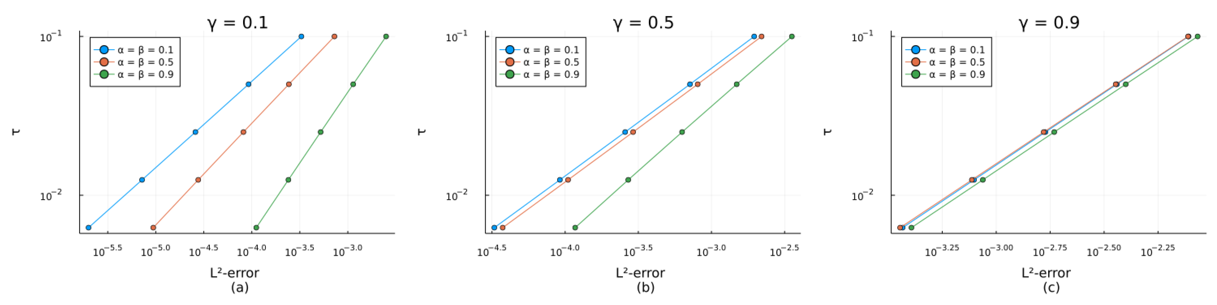
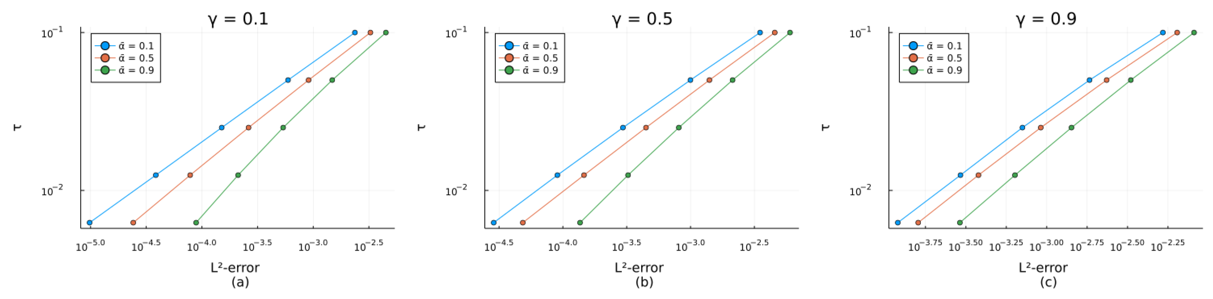
3.1. Verification of the Convergence Order

To verify the theoretical convergence estimates obtained in Theorems 3 and 4 for the fully discrete schemes, a number of computational experiments were carried out on the example of two model problems with known exact solutions. Numerical algorithms were implemented in FreeFEM++.

The purpose of the computational experiments carried out for Example 1 below was to determine the dependence of the empirical convergence order on orders of the fractional derivatives, and compare the empirical convergence order with the theoretical convergence order obtained in Theorem 3.

Example 1.

Consider the fractional differential equation

$${\partial }_{t}p+{\partial }_{0,t}^{\alpha }p+{\partial }_{0,t}^{\beta }p-{\partial }_{0,t}^{\gamma }{p}_{xx}=3x\left(x-1\right)\left(\frac{2t^{3-\alpha }}{\Gamma \left(1-\alpha \right)\left(\alpha -3\right)\left(\alpha -2\right)\left(\alpha -1\right)}\right.$$

$$+\left.\frac{2t^{3-\beta }}{\Gamma \left(1-\beta \right)\left(\beta -3\right)\left(\beta -2\right)\left(\beta -1\right)}-t^2\right)-\frac{12t^{3-\gamma }}{\Gamma \left(1-\gamma \right)\left(\gamma -3\right)\left(\gamma -2\right)\left(\gamma -1\right)},$$

$$x\in \Omega =\left(0,1\right),t\in \left(0,1\right]$$

subject to the following initial and boundary conditions:

$$p\left(x,0\right)=0,x\in \overline{\Omega },$$

$$p\left(0,t\right)=p\left(1,t\right)=0,t\in \left(0,1\right],$$

where $\alpha ,\beta ,\gamma \in \left(0,1\right)$. The exact solution of the problem is $p\left(x,t\right)=x\left(1-x\right)t^3$.

First, we studied the convergence behavior of the numerical solution with respect to the time step. Successively halving the time step in the range from $\tau =1/10$ to $\tau =1/160$ for a fixed number of elements M = 20,000, we calculated the corresponding errors $E_{\tau }$ in the $L^2$-norm and the convergence order by the formula

$$r=\frac{ln\left(E_{2\tau }/E_{\tau }\right)}{ln2}.$$

The choice of a relatively large M was motivated by the intention to reduce the influence of the error with respect to the spatial variable in this numerical test. Several combinations of the fractional derivative orders from the set $\left\{0.1,0.5,0.9\right\}$ were considered, and the values $\alpha$ and $\beta$ were assumed to be equal for simplicity.

The calculation results are presented in Table 1. In the ”Order“ column, the theoretical convergence orders are indicated in parentheses.

Table 1. $L^2$-errors and convergence orders obtained for Example 1 when h = 1/20,000. The numbers in parentheses indicate the theoretical convergence order.

$\mathit{\tau }$	$\mathit{\alpha }=\mathit{\beta }=0.1$		$\mathit{\alpha }=\mathit{\beta }=0.5$		$\mathit{\alpha }=\mathit{\beta }=0.9$
	${\mathit{L}}^2$-Error	Order	${\mathit{L}}^2$-Error	Order	${\mathit{L}}^2$-Error	Order
$\gamma =0.1$
$1/10$	$3.2849\times {10}^{-4}$	-	$7.2572\times {10}^{-4}$	-	$2.5025\times {10}^{-3}$	-
$1/20$	$9.2528\times {10}^{-5}$	1.83 (≃1.90)	$2.4325\times {10}^{-4}$	1.58 (≃1.50)	$1.1371\times {10}^{-3}$	1.14 (≃1.10)
$1/40$	$2.5876\times {10}^{-5}$	1.84 (≃1.90)	$8.1825\times {10}^{-5}$	1.57 (≃1.50)	$5.2122\times {10}^{-4}$	1.13 (≃1.10)
$1/80$	$7.1986\times {10}^{-6}$	1.85 (≃1.90)	$2.7674\times {10}^{-5}$	1.56 (≃1.50)	$2.4040\times {10}^{-4}$	1.12 (≃1.10)
$1/160$	$1.9943\times {10}^{-6}$	1.85 (≃1.90)	$9.4167\times {10}^{-6}$	1.56 (≃1.50)	$1.1134\times {10}^{-4}$	1.11 (≃1.10)
$\gamma =0.5$
$1/10$	$1.9588\times {10}^{-3}$	-	$2.2005\times {10}^{-3}$	-	$3.5455\times {10}^{-3}$	-
$1/20$	$7.1320\times {10}^{-4}$	1.46 (≃1.50)	$8.0528\times {10}^{-4}$	1.45 (≃1.50)	$1.4874\times {10}^{-3}$	1.25 (≃1.10)
$1/40$	$2.5706\times {10}^{-4}$	1.47 (≃1.50)	$2.9148\times {10}^{-4}$	1.47 (≃1.50)	$6.2996\times {10}^{-4}$	1.24 (≃1.10)
$1/80$	$9.2043\times {10}^{-5}$	1.48 (≃1.50)	$1.0471\times {10}^{-4}$	1.48 (≃1.50)	$2.6991\times {10}^{-4}$	1.22 (≃1.10)
$1/160$	$3.2809\times {10}^{-5}$	1.49 (≃1.50)	$3.7426\times {10}^{-5}$	1.48 (≃1.50)	$1.1708\times {10}^{-4}$	1.21 (≃1.10)
$\gamma =0.9$
$1/10$	$7.7892\times {10}^{-3}$	-	$7.7469\times {10}^{-3}$	-	$8.5795\times {10}^{-3}$	-
$1/20$	$3.6247\times {10}^{-3}$	1.10 (≃1.10)	$3.5794\times {10}^{-3}$	1.11 (≃1.10)	$3.9847\times {10}^{-3}$	1.11 (≃1.10)
$1/40$	$1.6908\times {10}^{-3}$	1.10 (≃1.10)	$1.6601\times {10}^{-3}$	1.11 (≃1.10)	$1.8576\times {10}^{-3}$	1.10 (≃1.10)
$1/80$	$7.8920\times {10}^{-4}$	1.10 (≃1.10)	$7.7124\times {10}^{-4}$	1.11 (≃1.10)	$8.6693\times {10}^{-4}$	1.10 (≃1.10)
$1/160$	$3.6836\times {10}^{-4}$	1.10 (≃1.10)	$3.5862\times {10}^{-4}$	1.10 (≃1.10)	$4.0467\times {10}^{-4}$	1.10 (≃1.10)

Error plots are shown in Figure 1.

Figure 1. Error plots with respect to the time step $\tau$ obtained for Example 1 with h = 1/20,000 and different orders of fractional derivatives: $\alpha \in \left\{0.1,0.5,0.9\right\}$; $\beta =\alpha$; (a) $\gamma =0.1$. (b) $\gamma =0.5$. (c) $\gamma =0.9$.

It follows from Table 1 that the convergence order with respect to the time step $\tau$ significantly depended on the orders of the fractional derivatives $\alpha ,\beta ,\gamma$. Specifically, it is easy to see that the empirical convergence order in $L^2$-norm was around 1.90 in case of $\alpha =\beta =\gamma =0.1$ and it decreased significantly with increasing order of the fractional derivatives. The convergence order was close to 1.10 when any of $\alpha ,\beta$ or $\gamma$ was equal to 0.9. This behavior agreed well with the theoretical order $O\left({\tau }^{2-\alpha }+{\tau }^{2-\beta }+{\tau }^{2-\gamma }\right)$.

In order to validate the convergence behavior with respect to the mesh size h, we fixed the time step $\tau$ = 1/20,000 and considered different values of the mesh size in the range from $h=1/5$ to $h=1/40$. The corresponding calculation results are presented in Table 2 and Figure 2.

Table 2. $L^2$-errors and convergence orders obtained for Example 1 when $\tau$ = 1/20,000. The numbers in parentheses indicate the theoretical convergence order.

h	$\mathit{\alpha }=\mathit{\beta }=0.1$		$\mathit{\alpha }=\mathit{\beta }=0.5$		$\mathit{\alpha }=\mathit{\beta }=0.9$
	${\mathit{L}}^2$-Error	Order	${\mathit{L}}^2$-Error	Order	${\mathit{L}}^2$-Error	Order
$\gamma =0.1$
$1/5$	$8.6774\times {10}^{-4}$	-	$1.0205\times {10}^{-3}$	-	$1.2214\times {10}^{-3}$	-
$1/10$	$2.2098\times {10}^{-4}$	1.97 (≃2.00)	$2.5958\times {10}^{-4}$	1.98 (≃2.00)	$3.1062\times {10}^{-4}$	1.98 (≃2.00)
$1/20$	$5.5494\times {10}^{-5}$	1.99 (≃2.00)	$6.5172\times {10}^{-5}$	1.99 (≃2.00)	$7.8361\times {10}^{-5}$	1.99 (≃2.00)
$1/40$	$1.3889\times {10}^{-5}$	2.00 (≃2.00)	$1.6315\times {10}^{-5}$	2.00 (≃2.00)	$2.0016\times {10}^{-5}$	1.97 (≃2.00)
$\gamma =0.5$
$1/5$	$6.0889\times {10}^{-4}$	-	$7.3163\times {10}^{-4}$	-	$8.9867\times {10}^{-4}$	-
$1/10$	$1.5537\times {10}^{-4}$	1.97 (≃2.00)	$1.8650\times {10}^{-4}$	1.97 (≃2.00)	$2.2911\times {10}^{-4}$	1.97 (≃2.00)
$1/20$	$3.9054\times {10}^{-5}$	1.99 (≃2.00)	$4.6867\times {10}^{-5}$	1.99 (≃2.00)	$5.7869\times {10}^{-5}$	1.99 (≃2.00)
$1/40$	$9.7935\times {10}^{-6}$	2.00 (≃2.00)	$1.1751\times {10}^{-5}$	2.00 (≃2.00)	$1.4824\times {10}^{-5}$	1.96 (≃2.00)
$\gamma =0.9$
$1/5$	$4.0575\times {10}^{-4}$	-	$4.9865\times {10}^{-4}$	-	$6.3234\times {10}^{-4}$	-
$1/10$	$1.0506\times {10}^{-4}$	1.95 (≃2.00)	$1.2865\times {10}^{-4}$	1.95 (≃2.00)	$1.6279\times {10}^{-4}$	1.96 (≃2.00)
$1/20$	$2.7770\times {10}^{-5}$	1.92 (≃2.00)	$3.3643\times {10}^{-5}$	1.94 (≃2.00)	$4.2397\times {10}^{-5}$	1.94 (≃2.00)
$1/40$	$7.3664\times {10}^{-6}$	1.91 (≃2.00)	$8.8056\times {10}^{-6}$	1.93 (≃2.00)	$1.1102\times {10}^{-5}$	1.93 (≃2.00)

Figure 2. Error plots with respect to the mesh size h obtained for Example 1 with $\tau$ = 1/20,000 and different orders of fractional derivatives: $\alpha \in \left\{0.1,0.5,0.9\right\}$; $\beta =\alpha$; (a) $\gamma =0.1$. (b) $\gamma =0.5$. (c) $\gamma =0.9$.

Table 2 shows that the spatial convergence order was close enough to 2.00 for all considered values of the fractional derivative orders, and therefore this result agreed well with Theorem 3. One can notice that the spatial convergence order decreased slightly as any of $\alpha ,\beta$ or $\gamma$ approached 1. This can be explained by the influence of the error with respect to the time step due to an insufficiently small value of $\tau$, $\tau$ = 1/20,000, and the fact that the temporal convergence order was around 1 in this case.

Thus, it can be concluded that the numerical results conducted for Example 1 fully confirmed the theoretically predicted convergence order obtained in Theorem 3.

Similarly, the purpose of the computational experiments carried out for Example 2 below was to compare the empirical convergence order with the theoretical convergence order obtained in Theorem 4. The numerical tests were mainly aimed at validating the convergence order with respect to the time step $\tau$. We considered different values of $\tau$ in the range from $1/10$ to $1/160$ with a fixed mesh size h = 1/40,000.

Example 2.

Consider the fractional differential equation

$${\partial }_{t}p+{\partial }_{0,t}^{\overline{\alpha }}\left({\partial }_{t}p+p\right)-\frac{1}{8}{\partial }_{0,t}^{\gamma }\left({\partial }_t{p}_{xx}+p_{xx}\right)$$

$$=-2tsin\left(\pi x\right)\left(\frac{t^{-\overline{\alpha }}\left(\overline{\alpha }-t-2\right)}{\Gamma \left(1-\overline{\alpha }\right)\left(\overline{\alpha }-2\right)\left(\overline{\alpha }-1\right)}+\frac{{\pi }^2{t}^{-\gamma }\left(\gamma -t-2\right)}{8\Gamma \left(1-\gamma \right)\left(\gamma -2\right)\left(\gamma -1\right)}-1\right),$$

$$x\in \Omega =\left(0,1\right),t\in \left(0,1\right]$$

subject to the following initial and boundary conditions:

$$p\left(x,0\right)={\partial }_{t}p\left(x,0\right)=0,x\in \overline{\Omega };$$

$$p\left(0,t\right)=p\left(1,t\right)=0,t\in \left(0,1\right],$$

where $\overline{\alpha },\gamma \in \left(0,1\right)$. The exact solution of the problem is $p\left(x,t\right)=t^{2}sin\left(\pi x\right)$.

In the experiments, several combinations of the fractional derivative orders $\overline{\alpha }$ and $\gamma$ from the set $\left\{0.1,0.5,0.9\right\}$ were considered. The results of the computational experiments are presented in Table 3 and error plots are shown in Figure 3.

Table 3. $L^2$-errors and convergence orders obtained for Example 2 when h = 1/40,000. The numbers in parentheses indicate the theoretical convergence order.

$\mathit{\tau }$	$\overline{\mathit{\alpha }}=0.1$		$\overline{\mathit{\alpha }}=0.5$		$\overline{\mathit{\alpha }}=0.9$
	${\mathit{L}}^2$-Error	Order	${\mathit{L}}^2$-Error	Order	${\mathit{L}}^2$-Error	Order
$\gamma =0.1$
$1/10$	$2.3676\times {10}^{-3}$	-	$3.2628\times {10}^{-3}$	-	$4.4958\times {10}^{-3}$	-
$1/20$	$5.9378\times {10}^{-4}$	2.00 (≃1.90)	$9.0842\times {10}^{-4}$	1.84 (≃1.50)	$1.4817\times {10}^{-3}$	1.60 (≃1.10)
$1/40$	$1.5068\times {10}^{-4}$	1.98 (≃1.90)	$2.6240\times {10}^{-4}$	1.79 (≃1.50)	$5.3666\times {10}^{-4}$	1.47 (≃1.10)
$1/80$	$3.8539\times {10}^{-5}$	1.97 (≃1.90)	$7.8441\times {10}^{-5}$	1.74 (≃1.50)	$2.1149\times {10}^{-4}$	1.34 (≃1.10)
$1/160$	$9.7984\times {10}^{-6}$	1.98 (≃1.90)	$2.4172\times {10}^{-5}$	1.70 (≃1.50)	$8.8729\times {10}^{-5}$	1.25 (≃1.10)
$\gamma =0.5$
$1/10$	$3.5044\times {10}^{-3}$	-	$4.5686\times {10}^{-3}$	-	$6.0144\times {10}^{-3}$	-
$1/20$	$9.9782\times {10}^{-4}$	1.81 (≃1.50)	$1.4057\times {10}^{-3}$	1.70 (≃1.50)	$2.1346\times {10}^{-3}$	1.49 (≃1.10)
$1/40$	$2.9554\times {10}^{-4}$	1.76 (≃1.50)	$4.4784\times {10}^{-4}$	1.65 (≃1.50)	$8.0921\times {10}^{-4}$	1.40 (≃1.10)
$1/80$	$9.0569\times {10}^{-5}$	1.71 (≃1.50)	$1.4635\times {10}^{-4}$	1.61 (≃1.50)	$3.2397\times {10}^{-4}$	1.32 (≃1.10)
$1/160$	$2.8713\times {10}^{-5}$	1.66 (≃1.50)	$4.8539\times {10}^{-5}$	1.59 (≃1.50)	$1.3629\times {10}^{-4}$	1.25 (≃1.10)
$\gamma =0.9$
$1/10$	$5.2340\times {10}^{-3}$	-	$6.4114\times {10}^{-3}$	-	$8.1559\times {10}^{-3}$	-
$1/20$	$1.8406\times {10}^{-3}$	1.51 (≃1.10)	$2.3477\times {10}^{-3}$	1.45 (≃1.10)	$3.3127\times {10}^{-3}$	1.30 (≃1.10)
$1/40$	$7.0754\times {10}^{-4}$	1.38 (≃1.10)	$9.1878\times {10}^{-4}$	1.35 (≃1.10)	$1.4232\times {10}^{-3}$	1.22 (≃1.10)
$1/80$	$2.9274\times {10}^{-4}$	1.27 (≃1.10)	$3.7822\times {10}^{-4}$	1.28 (≃1.10)	$6.3606\times {10}^{-4}$	1.16 (≃1.10)
$1/160$	$1.1989\times {10}^{-4}$	1.29 (≃1.10)	$1.6027\times {10}^{-4}$	1.24 (≃1.10)	$2.9034\times {10}^{-4}$	1.13 (≃1.10)

Figure 3. Error plots with respect to the time step $\tau$ obtained for Example 2 with h = 1/40,000 and different orders of fractional derivatives: $\overline{\alpha }\in \left\{0.1,0.5,0.9\right\}$; (a) $\gamma =0.1$. (b) $\gamma =0.5$. (c) $\gamma =0.9$.

Making a comparison of empirical and theoretical convergence orders presented in Table 3, one may conclude that the numerical results fully confirmed the theoretical prediction obtained in Theorem 4.

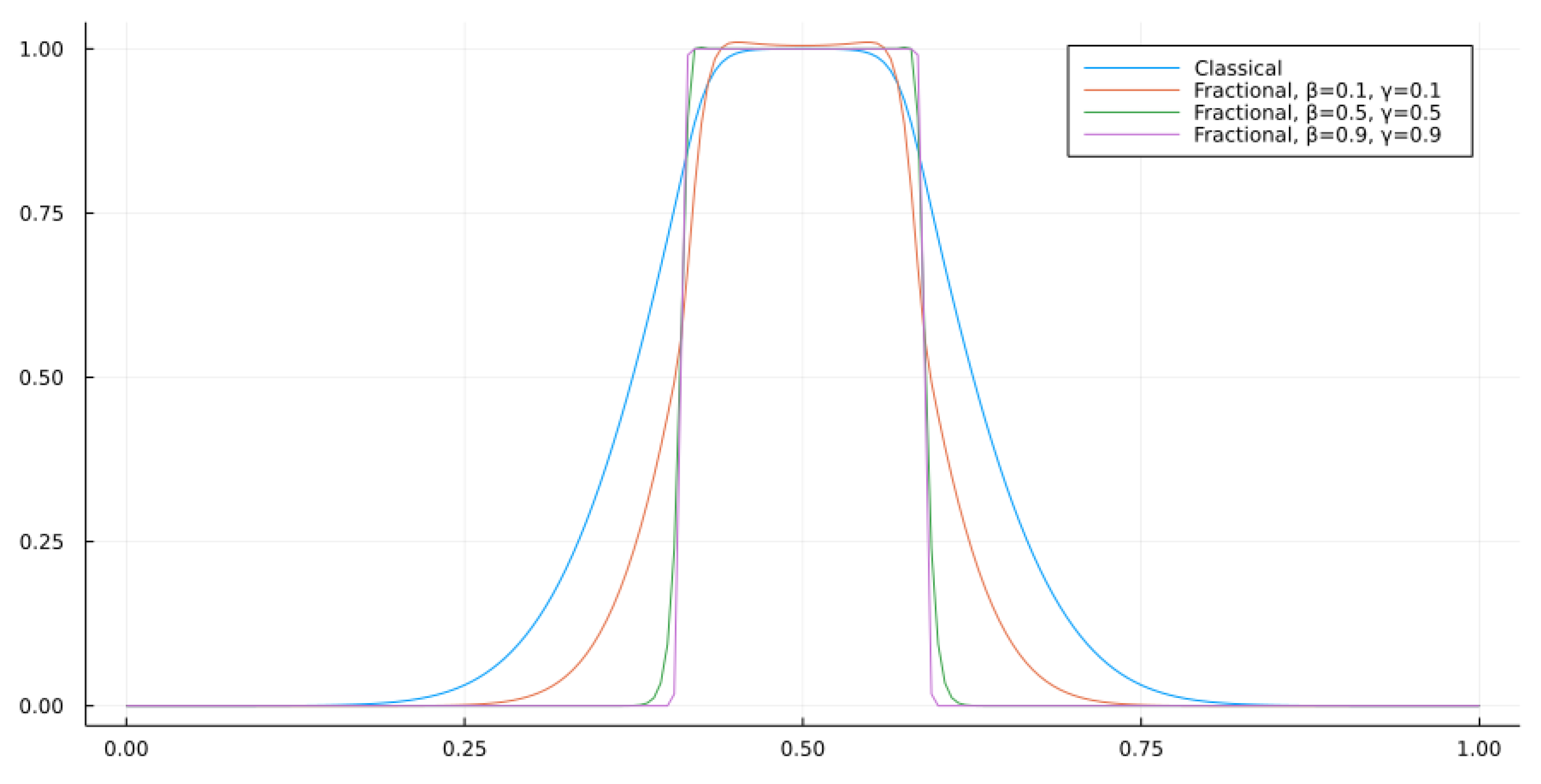
3.2. Verification of the Model

Now we examine the proposed numerical method (43), (44) to solve a more realistic example. Let us consider the process of oil flow in a fractured porous medium. We considered the case when the influence of porosity changes on the fluid flow process could be neglected, i.e., $\varphi =\mathrm{const}$. Further, we chose the constant $\mu$ in Assumption 2 to be equal to ${\displaystyle \mu =\frac{k}{\tilde{\mu }}}$ and restricted ourselves to the case $\overline{\beta }\in \left(-1,0\right)$. In this case, equation (8) was reduced to the following form:

$$\varphi c_{f1}{\partial }_{t}p+\varphi c_{f\overline{\beta }}{\partial }_{0,t}^{\overline{\beta }+1}p-\frac{k}{\tilde{\mu }}{\partial }_{0,t}^{\gamma }{p}_{xx}={\overline{f}}_0,x\in \Omega \equiv \left(0,l_0\right),t>0.$$

(66)

Supplement the Equation (66) with the initial condition $p\left(x,0\right)=p_0\left(x\right)$, $x\in \overline{\Omega }$ and homogeneous boundary conditions which corresponds to the case when two production wells are placed at the ends of the segment $\overline{\Omega }$. We choose the right-hand side ${\overline{f}}_0$ in the form

$${\overline{f}}_0=\frac{2\pi kH}{\tilde{\mu }lnr}\left(p_{bh}-p\right)\delta \left(x-x_0\right),$$

where $p_{bh}$ is a predetermined pressure value, H is the thickness of the reservoir, $p_{bh}>p$, $x_0\in \Omega$, $\delta \left(x\right)$ is the delta function, and r is a value determined by the radius of the borehole. Let us introduce the dimensionless parameters

$$\overline{t}=\frac{t}{\lambda },\lambda =\frac{k_0\left(p_{bh}-p_0\right)}{\varphi {\mu }_0{l}_0^2},\overline{x}=\frac{x}{l_0},\overline{\rho }=\frac{\rho }{{\rho }_0},\overline{\mu }=\frac{\tilde{\mu }}{{\mu }_0},\overline{p}=\frac{p-p_0}{p_{bh}-p_0},\overline{k}=\frac{k}{k_0}.$$

By using the fact that

$${\partial }_{0,\overline{t}}^{\nu }p\left(\overline{t}\right)={\lambda }^{\nu }{\partial }_{0,t}^{\nu }p\left(t\right),$$

the Equation (66) is reduced to the form

$${\overline{c}}_{f1}\frac{\partial \overline{p}}{\partial \overline{t}}+{\overline{c}}_{f\overline{\beta }}{\partial }_{0,\overline{t}}^{\overline{\beta }+1}\overline{p}-\frac{\overline{k}{\lambda }^{\gamma }}{\overline{\mu }}{\partial }_{0,\overline{t}}^{\gamma }{\overline{p}}_{xx}=c_0{\overline{f}}_0,x\in {\Omega }_1\equiv \left(0,1\right),\overline{t}>0,$$

(67)

where ${\overline{c}}_{f1}=\frac{1}{\overline{\rho }}\frac{\partial \overline{\rho }}{\partial \overline{p}}$, ${\overline{c}}_{f\overline{\beta }}=\frac{1}{\overline{\rho }}\frac{\partial \overline{\rho }}{\partial \left({\partial }_{0,\overline{t}}^{\overline{\beta }}\overline{p}\right)}$, ${\overline{c}}_0=\frac{{\mu }_0{l}_0^2}{k_0\left(p_{bh}-p_c\right)}$ and is supplemented by the initial and boundary conditions

$$\overline{p}\left(x,0\right)={\overline{p}}_0\left(\overline{x}\right),\overline{x}\in {\overline{\Omega }}_1,$$

(68)

$$\overline{p}\left(0,\overline{t}\right)=\overline{p}\left(1,\overline{t}\right)=0,\overline{t}>0.$$

(69)

Now, using the Equations (1) and (2) and the classical state equation $\rho =\rho \left(p\right)$, we obtain the following classical fluid flow equation describing flow in a continuous porous medium:

$${\overline{c}}_{f1}\frac{\partial \overline{p}}{\partial \overline{t}}-\frac{\overline{k}}{\overline{\mu }}{\overline{p}}_{xx}=c_0{\overline{f}}_0.$$

(70)

The goal of the numerical tests was to compare the solutions of the Equations (67) and (70) subject to the initial and boundary conditions (68), (69) in order to verify the model (8) of fluid flow in fractured porous media. The numerical tests were conducted using the following values of the dimensionless parameters: ${\overline{p}}_{bh}=1$, ${\overline{p}}_0\left(x\right)=0$, $\overline{k}=2\times {10}^{-6}$, $\overline{\mu }=0.0895$, ${\overline{c}}_{f1}=0.0019$, ${\overline{c}}_{f\overline{\beta }}=4\times {10}^{-6}$. The results of the numerical tests are presented in Figure 4.

Figure 4. The result of comparison of the classical model of fluid flow in porous media with the fractional model (8) for various orders of the fractional derivatives at $\overline{t}=0.5$.

Let us recall that the motion law (6) is suitable for describing the process of fluid flow in fractured porous media with the uniformly distributed fractures over the volume [6]. Figure 4 shows a deceleration of the process of fluid flow, and it can be clearly seen that an increase in the orders of the fractional derivative led to a greater deceleration. This behavior confirmed the fact that the porous medium had a retarding effect on the flow process, and the orders of the fractional derivatives determined the degree of memory impact on patterns of the flow.

4. Discussion

Thus, having carried out a theoretical analysis of the constructed numerical methods and having analyzed the results of the computational experiments, the following conclusions can be outlined.

(1) Both computational methods constructed for solving Problem 1 in the special cases $\overline{\alpha },\overline{\beta }\in \left(-1,0\right)$, $\gamma \in \left(0,1\right)$ and $\overline{\alpha },\gamma \in \left(0,1\right)$, $\overline{\beta }=\overline{\alpha }-1$ (or $\overline{\beta },\gamma \in \left(0,1\right)$, $\overline{\alpha }=\overline{\beta }-1$) allow obtaining an approximate solution with the second order of accuracy in the spatial direction and an order of $2-\nu$ with respect to the temporal variable, where $\nu$ is the largest of the fractional derivative orders. The results of computational experiments conducted for various orders of the fractional derivatives and grid configurations fully confirm the results of the theoretical analysis.

(2) Based on the results of the numerical tests presented in Section 3.2, we conclude that the model under study reproduces the characteristic features of the process of fluid flow in a fractured porous medium. In particular, the test carried out within the framework of the studied model showed that the fluid flow process in a fractured porous medium proceeds more slowly than in a continuous medium. This observation is also consistent with the conclusions of the paper [8].

In subsequent papers, the authors intend to consider the initial boundary value problem for the Equation (7) with a more general form of the function $\mathcal{F}$. Specifically, more realistic examples of fluid flow problems in a fractured porous medium will be considered, and a more extensive comparison of the simulation results with the results of similar works will be carried out.

(3) Since this is the first work devoted to the numerical implementation of the model under consideration, the authors restricted themselves to constructing numerical schemes of nearly second order of convergence. The results obtained can be improved by using higher-order approximations of the Caputo fractional derivative (see, for example, [38,51]). A separate paper will be devoted to this study.

(4) The conclusions obtained in this study can be used in solving other classes of fractional differential equations. The results of the presented work will also form the basis for further research in this direction. For example, a natural continuation of our work is the study of multi-dimensional models of fluid flow in a fractured porous medium with fractal geometry of fractures and models of single-phase fluid flow with spatial fractional derivatives.

References

1. Hoteit, H.; Firoozabadi, A. An Efficient Numerical Model for Incompressible Two-phase Flow in Fractured Media. Adv. Water Resour. 2008, 31, 891–905. [Google Scholar] [CrossRef]
2. Berre, I.; Doster, F.; Keilegavlen, E. Flow in Fractured Porous Media: A Review of Conceptual Models and Discretization Approaches. Transp. Porous Media 2019, 130, 215–236. [Google Scholar] [CrossRef] [Green Version]
3. Lee, J.; Choi, S.-U.; Cho, W. A Comparative Study of Dual-Porosity Model and Discrete Fracture Network Model. Water Eng. 1999, 3, 171–180. [Google Scholar] [CrossRef]
4. Moinfar, A.; Narr, W.; Hui, M.-H.; Mallison, B.; Lee, S.H. Comparison of Discrete-Fracture and Dual-Permeability Models for Multiphase Flow in Naturally Fractured Reservoirs. In Proceedings of the SPE Reservoir Simulation Symposium, The Woodlands, TX, USA, 21–23 February 2011; Abstract Number SPE 142295. pp. 1–17. [Google Scholar]
5. Torres, F.; Xavier, M.; Ailin, J.; Wei, Y.; Yunsheng, W.; Junlei, W.; Xie, H.; Li, N.; Miao, J. Comparison of Dual Porosity Dual Permeability with Embedded Discrete Fracture Model for Simulation Fluid Flow in Naturally Fractured Reservoirs. In Proceedings of the 54th U.S. Rock Mechanics/Geomechanics Symposium, Golden, CO, USA, 28 June–1 July 2020. Abstract Number ARMA-2020-1462. [Google Scholar]
6. Gazizov, R.K.; Lukashchuk, S.Y. Fractional Differential Approach to Modeling Filtration Processes in Complex Inhomogeneous Porous Media. Vestnik UGATU 2017, 21, 104–112. (In Russian) [Google Scholar]
7. Zhong, W.; Li, C.; Kou, J. Numerical Fractional-Calculus Model for Two-Phase Flow in Fractured Media. Adv. Math. Phys. 2013, 2013, 429835. [Google Scholar] [CrossRef]
8. Beybalaev, V.D.; Abduragimov, E.I.; Yakubov, A.Z.; Meilanov, R.R.; Aliverdiev, A.A. Numerical Research of Non-Isothermal Filtration Process in Fractal Medium with Non-Locality in Time. Therm. Sci. 2021, 25, 465–475. [Google Scholar] [CrossRef] [Green Version]
9. Caputo, M. Models of Flux in Porous Media with Memory. Water Resour. Res. 2000, 36, 693–705. [Google Scholar] [CrossRef]
10. Hossain, M.E. Numerical Investigation of Memory-Based Diffusivity Equation: The Integro-Differential Equation. Arab. J. Sci. Eng. 2016, 41, 1–15. [Google Scholar] [CrossRef]
11. Di Giuseppe, E.; Moroni, M.; Caputo, M. Flux in Porous Media with Memory: Models and Experiments. Transp. Porous Media 2010, 83, 479–500. [Google Scholar] [CrossRef]
12. Caffarelli, L.; Vazquez, J.L. Nonlinear Porous Medium Flow with Fractional Potential Pressure. Arch. Ration. Mech. Anal. 2011, 202, 537–565. [Google Scholar] [CrossRef] [Green Version]
13. Gazizov, R.K.; Kasatkin, A.A.; Lukashchuk, S.Y. Symmetries and Exact Solutions of Fractional Filtration Equations. AIP Conf. Proc. 2017, 1907, 020010. [Google Scholar]
14. Meilanov, R.R.; Akhmedov, E.N.; Beybalaev, V.D.; Magomedov, R.A.; Ragimkhanov, G.B.; Aliverdiev, A.A. To the Theory of Non-Local Non-Isothermal Filtration in Porous Medium. J. Phys. Conf. Ser. 2018, 946, 012076. [Google Scholar] [CrossRef]
15. Hashan, M.; Jahan, L.N.; Zaman, T.U.; Imtiaz, S.; Hossain, M.E. Modelling of Fluid Flow Through Porous Media Using Memory Approach: A Review. Math. Comput. Simul. 2020, 177, 643–673. [Google Scholar] [CrossRef]
16. Li, J.; Jiang, T.Q. Constitutive Equation for Viscoelastic Fluids via Fractional Derivative; Allerton Press: New York, NY, USA, 1994. [Google Scholar]
17. He, J.H. Approximate Analytical Solution for Seepage Flow with Fractional Derivatives in Porous Media. Comput. Methods Appl. Mech. Eng. 1998, 167, 57–88. [Google Scholar] [CrossRef]
18. Oliveira, E.; Machado, J. A Review of Definitions for Fractional Derivatives and Integral. Math. Probl. Eng. 2014, 2014, 238459. [Google Scholar] [CrossRef] [Green Version]
19. Teodoro, G.; Machado, J.; Oliveira, E. A Review of Definitions of Fractional Derivatives and Other Operators. J. Comput. Phys. 2019, 388, 195–208. [Google Scholar] [CrossRef]
20. Bohaienko, V.; Bulavatsky, V. Mathematical Modeling of Solutes Migration Under the Conditions of Groundwater Filtration by the Model with the K-Caputo Fractional Derivative. Fractal Fract. 2018, 2, 28. [Google Scholar] [CrossRef] [Green Version]
21. Atangana, A. Fractional Operators with Constant and Variable Order with Application to Geo-Hydrology; Elsevier: Amsterdam, The Netherlands, 2018. [Google Scholar]
22. Prajapati, J.C.; Patel, A.D.; Pathak, K.N.; Shukla, A.K. Fractional Calculus Approach in the Study of Instability Phenomenon in Fluid Dynamics. Palest. J. Math. 2012, 1, 95–103. [Google Scholar]
23. Agarwal, R.; Yadav, M.P.; Baleanu, D.; Purohit, S.D. Existence and Uniqueness of Miscible Flow Equation Through Porous Media with a Non Singular Fractional Derivative. AIMS Math. 2020, 5, 1062–1073. [Google Scholar] [CrossRef]
24. Zhou, H.W.; Yang, S.; Zhang, S.Q. Modeling of Non-Darcian Flow and Solute Transport in Porous Media with Caputo-Fabrizio Derivative. Appl. Math. Model. 2019, 68, 603–615. [Google Scholar] [CrossRef]
25. Wei, Q.; Zhou, H.; Yang, S. Non-Darcy flow Models in Porous Media via Atangana-Baleanu Derivative. Chaos Solitons Fractals 2020, 141, 110335. [Google Scholar] [CrossRef]
26. Al-Homidan, S.; Ghanam, R.A.; Tatar, N. On a Generalized Diffusion Equation Arising in Petroleum Engineering. Adv. Differ. Equ. 2013, 2013, 349. [Google Scholar] [CrossRef] [Green Version]
27. Chang, A.; Sun, H.; Zhang, Y.; Zheng, C.; Min, F. Spatial Fractional Darcy’s Law to Quantify Fluid Flow in Natural Reservoirs. Phys. A Stat. Mech. Its Appl. 2019, 519, 119–126. [Google Scholar] [CrossRef]
28. Heymans, N.; Podlubny, I. Physical Interpretation of Initial Conditions for Fractional Differential Equations with Riemann-Liouville Fractional Derivatives. Rheol Acta 2006, 45, 765–771. [Google Scholar] [CrossRef] [Green Version]
29. Tarasov, V.E. Caputo-Fabrizio Operator in Terms of Integer Derivatives: Memory or Distributed Lag? Comput. Appl. Math. 2019, 38, 113. [Google Scholar] [CrossRef]
30. El Amin, M.F.; Radwan, A.G.; Sun, S. Analytical Solution for Fractional Derivative Gas-Flow Equation in Porous Media. Results Phys. 2017, 7, 2432–2438. [Google Scholar] [CrossRef] [Green Version]
31. Ray, S.S. Exact Solutions for Time-Fractional Diffusion-Wave Equations by Decomposition Method. Phys. Scr. 2007, 75, 53–61. [Google Scholar] [CrossRef]
32. Zhang, Y.N.; Sun, Z.Z.; Liao, H.L. Finite Difference Methods for the Time Fractional Diffusionequation on Non-Uniform Meshes. J. Comput. Phys. 2014, 265, 195–210. [Google Scholar] [CrossRef]
33. Qiao, H.L.; Liu, Z.G.; Cheng, A.J. Two Unconditionally Stable Difference Schemes for Time Distributed-Order Differential Equation Based on Caputo–Fabrizio Fractional Derivative. Adv. Differ. Equ. 2020, 2020, 1–17. [Google Scholar] [CrossRef]
34. Alimbekova, N.B.; Berdyshev, A.S.; Baigereyev, D.R. Parallel Implementation of the Algorithm for Solving a Partial Differential Equation with a Fractional Derivative in the Sense of Riemann-Liouville. In Proceedings of the 2021 IEEE International Conference on Smart Information Systems and Technologies (SIST), Nur-Sultan, Kazakhstan, 28–30 April 2021; pp. 1–6. [Google Scholar] [CrossRef]
35. Du, R.; Cao, W.R.; Sun, Z.Z. A Compact Difference Scheme for the Fractional Diffusion-Wave Equation. Appl. Math. Model. 2010, 34, 2998–3007. [Google Scholar] [CrossRef]
36. Huang, J.; Tang, Y.; Wang, W.; Yang, J. A Compact Difference Scheme for Time Fractional Diffusion Equation with Neumann Boundary Conditions. Commun. Comput. Inf. Sci. 2012, 323, 273–284. [Google Scholar]
37. Xu, T.; Lu, S.; Chen, W.; Chen, H. Finite Difference Scheme for Multi-term Variable-order Fractional Diffusion Equation. Adv. Differ. Equ. 2018, 1, 1–13. [Google Scholar] [CrossRef] [Green Version]
38. Alikhanov, A.A. A New Difference Scheme for the Time Fractional Diffusion Equation. J. Comput. Phys. 2015, 280, 424–438. [Google Scholar] [CrossRef] [Green Version]
39. Liu, J.; Zhou, Z. Finite Element Approximation of Time Fractional Optimal Control Problem with Integral State Constraint. AIMS Math. 2020, 6, 979–997. [Google Scholar] [CrossRef]
40. Zhang, C.; Liu, H.; Zhou, Z.J. A Priori Error Analysis for Time-Stepping Discontinuous Galerkin Finite Element Approximation of Time Fractional Optimal Control Problem. J. Sci. Comput. 2019, 80, 993–1018. [Google Scholar] [CrossRef]
41. Liu, K.; Feckan, M.; O’Regan, D.; Wang, J.R. Hyers–Ulam Stability and Existence of Solutions for Differential Equations with Caputo–Fabrizio Fractional Derivative. Mathematics 2019, 7, 333. [Google Scholar] [CrossRef] [Green Version]
42. Liu, Y.; Du, Y.; Li, H.; Li, J.; He, S. A Two-Grid Mixed Finite Element Method for a Nonlinear Fourth-Order Reaction-Diffusion Problem with Time-Fractional Derivative. Comput. Math. Appl. 2015, 70, 2474–2492. [Google Scholar] [CrossRef]
43. Liu, F.; Zhuang, P.; Turner, I.; Burrage, K.; Anh, V. A New Fractional Finite Volume Method for Solving the Fractional Diffusion Equation. Appl. Math. Model. 2014, 38, 3871–3878. [Google Scholar] [CrossRef]
44. Wang, H.; Cheng, A.; Wang, K. Fast Finite Volume Methods for Space-fractional Diffusion Equations. Discret. Contin. Dyn. Syst. Ser. B 2015, 20, 1427–1441. [Google Scholar] [CrossRef]
45. Mallawi, F.; Alzaidy, J.F.; Hafez, R.M. Application of a Legendre Collocation Method to the Space-time Variable Fractional-order Advection-dispersion Equation. J. Taibah Univ. Sci. 2019, 13, 324–330. [Google Scholar] [CrossRef] [Green Version]
46. Oldham, K.B.; Spanier, J. The Fractional Calculus; Academic Press: New York, NY, USA, 1974. [Google Scholar]
47. Lin, Y.; Xu, C. Finite Difference/Spectral Approximations for the Time-Fractional Diffusion Equation. J. Comput. Phys. 2007, 225, 1533–1552. [Google Scholar] [CrossRef]
48. Jin, B.; Lazarov, R.; Zhou, Z. An Analysis of the L1 Scheme for the Subdiffusion Equation with Nonsmooth Data. IMA J. Numer. Anal. 2016, 36, 197–221. [Google Scholar] [CrossRef] [Green Version]
49. Yan, Y.; Khan, M.; Ford, N. An Analysis of the Modified L1 Scheme for Time-fractional Partial Differential Equations with Nonsmooth Data. SIAM J. Numer. Anal. 2018, 56, 210–227. [Google Scholar] [CrossRef]
50. Siddiqi, S.; Arshed, S. Numerical Solution of Time-fractional Fourth-order Partial Differential Equations. Int. J. Comput. Math. 2015, 92, 1496–1518. [Google Scholar] [CrossRef]
51. Gao, G.H.; Sun, Z.Z.; Zhang, H.W. A New Fractional Numerical Differentiation Formula to Approximate the Caputo Fractional Derivative and Its Applications. J. Comput. Phys. 2014, 259, 33–50. [Google Scholar] [CrossRef]
52. Cao, J.; Li, C.; Chen, Y. High-order Approximation to Caputo Derivatives and Caputo-type Advection-Diffusion Equation (II). Fract. Calc. Appl. Anal. 2015, 18, 735–761. [Google Scholar] [CrossRef]
53. Xuhao, L. Numerical Methods for Fractional Differential Equations. Ph.D. Thesis, Nanyang Technological University, Singapore, 2018. [Google Scholar]
54. Atangana, A. Extension of Rate of Change Concept: From Local to Nonlocal Operators with Applications. Results Phys. 2020, 19, 103515. [Google Scholar] [CrossRef]
55. Ouyang, Y.; Wang, W. Comparison of Definition of Several Fractional Derivatives. In Proceedings of the 2016 6th International Conference on Education, Management and Computer Science (ICEMC 2016), Shenyang, China, 27–29 May 2016; pp. 553–557. [Google Scholar]
56. Prieur, F.; Holm, S. Nonlinear Acoustic Wave Equations with Fractional Loss Operators. J. Acoust. Soc. Am. 2011, 130, 1125–1132. [Google Scholar] [CrossRef] [Green Version]
57. Adams, R. Sobolev Spaces; Academic Press: New York, NY, USA, 1975. [Google Scholar]
58. Brezzi, F.; Fortin, M. Mixed and Hybrid Finite Element Methods; Springer: New York, NY, USA, 1991. [Google Scholar]