
On the Modelling of Emergency Ambulance Trips: The Case of the Žilina Region in Slovakia


Abstract
:1. Introduction
1.1. Literature Review
1.2. The Scientific Contributions and Structure of the Paper
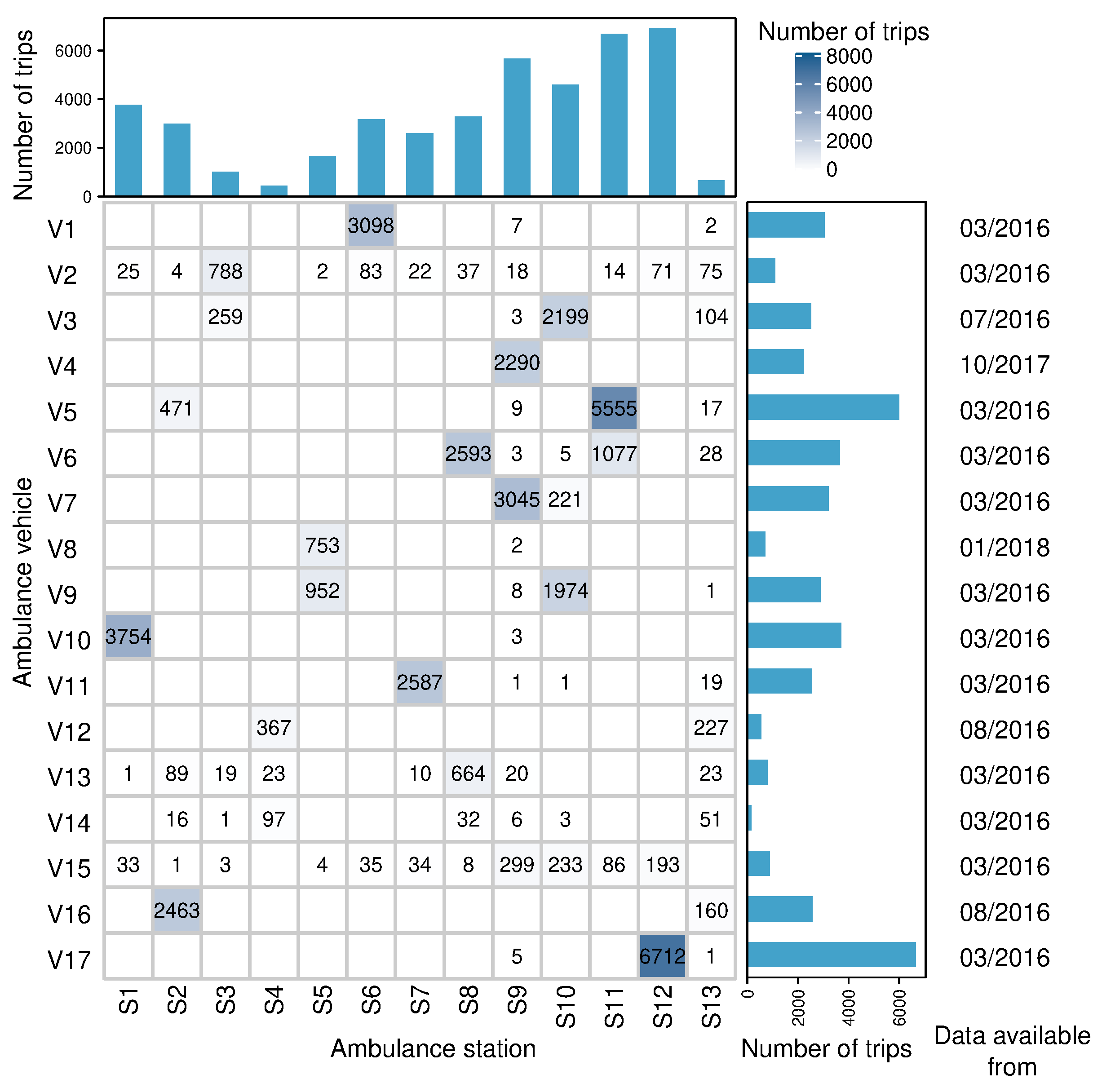
2. Materials
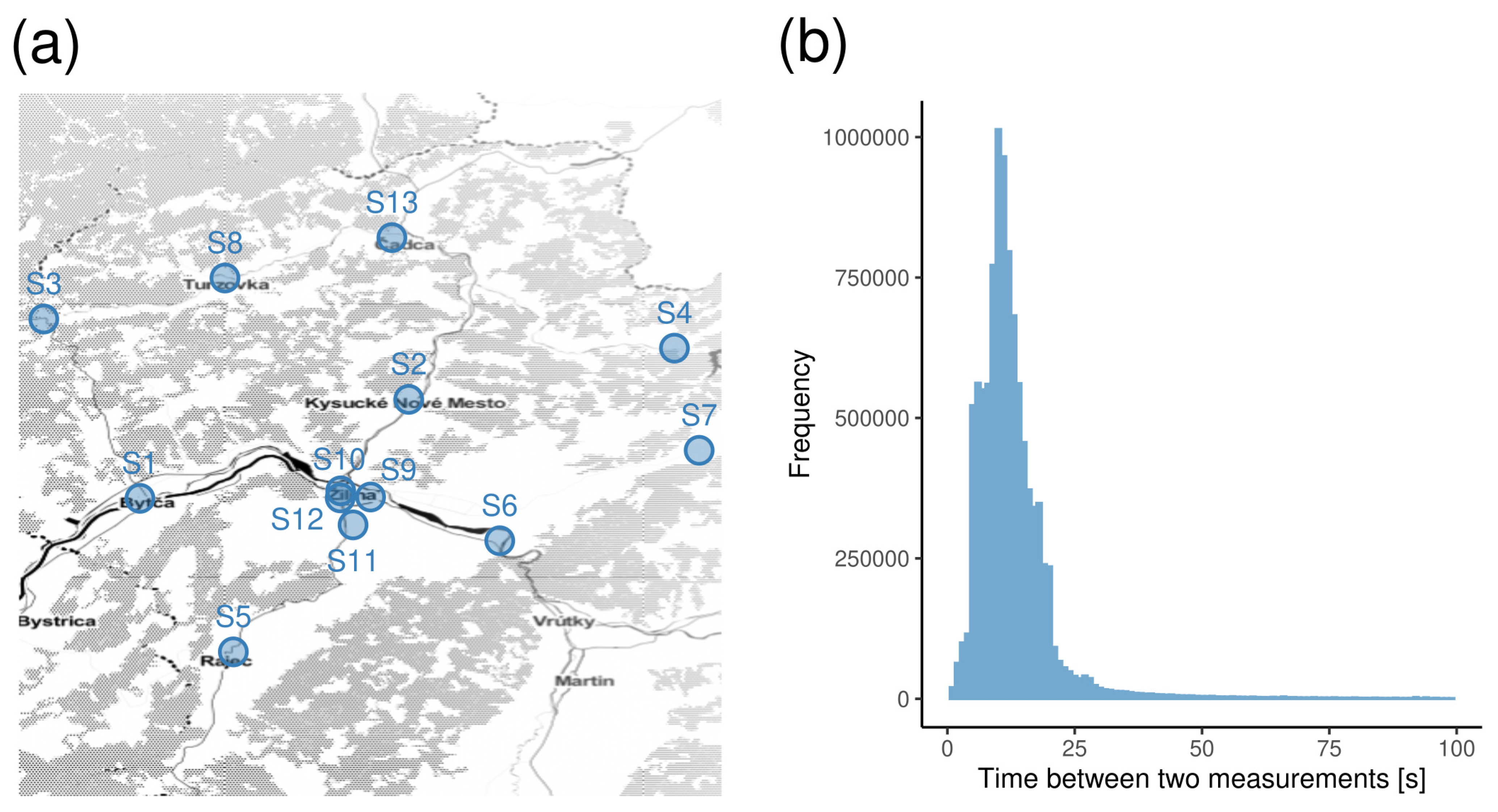
Falck Dataset
3. Methods
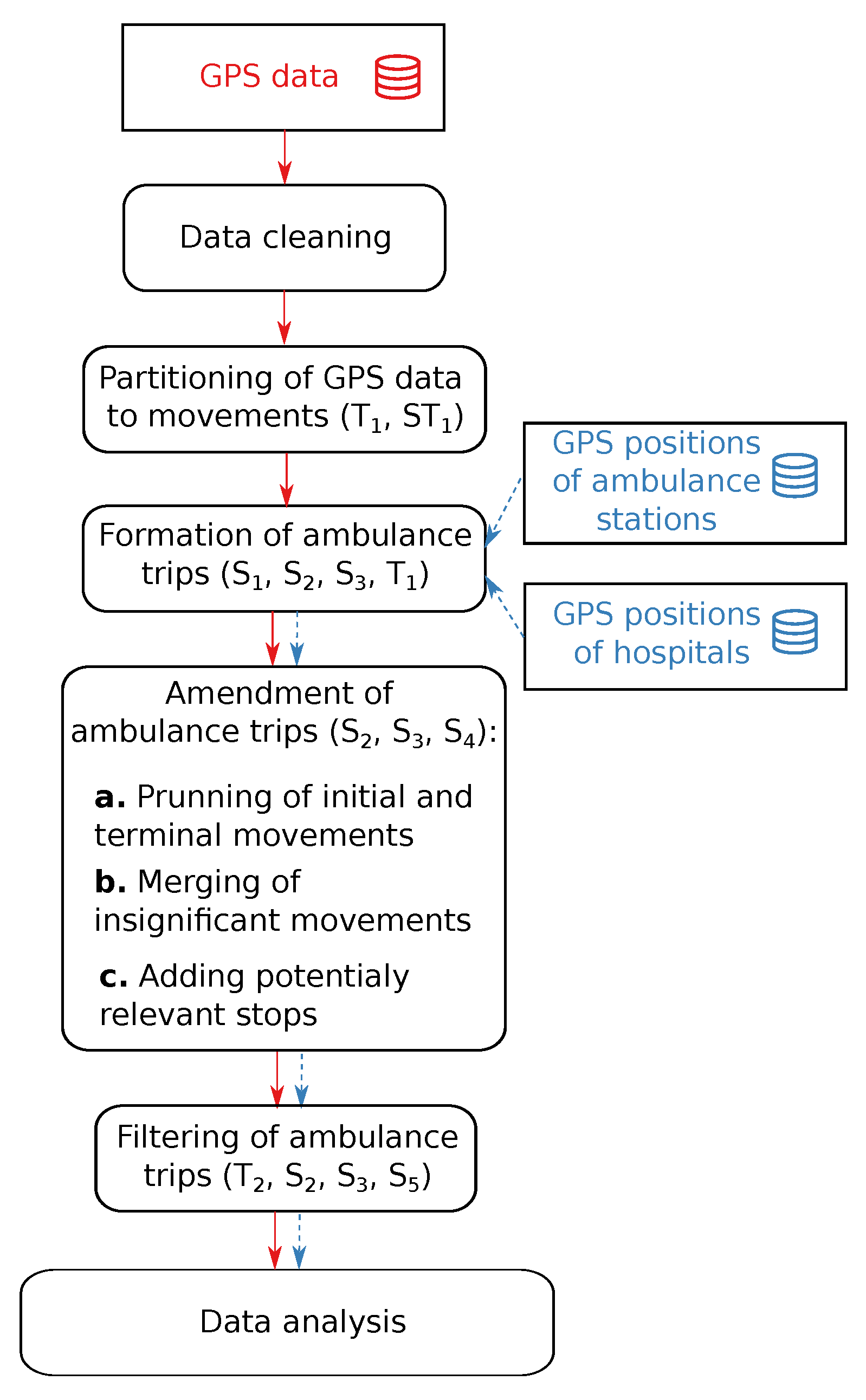
3.1. Data Pre-Processing Workflow
- Time between two consecutive GPS-based measurements ();
- Overall duration of the trip ();
- Aerial distance between two consecutive GPS-based measurements ();
- Aerial distance between an initial (terminal) GPS-based measurements of a movement and a hospital ();
- Aerial distance between an initial (terminal) GPS-based measurements of a movement and an ambulance station ();
- Length of a movement ();
- Overall length of a trip ();
- Instantaneous speed ().
- Data cleaning: In this phase, typical data problems such as empty, unexpected, or redundant values were handled. Whenever possible, the data problems were fixed; e.g., values of categorical features such as the state of the blue lights and siren were unified. Problematic data, such as redundant table rows, were eliminated. As the data analysis focuses only on three administrative districts located in the Žilina region, the records corresponding to the ambulance leaving the area of the Slovak Republic were eliminated. Similarly, whenever we identified from the data that an ambulance was operated from a station in a different Slovak region, we excluded the corresponding records from the analysis. This occurred when the operator decided to allocate an ambulance to another area temporarily. Moreover, we analysed the average velocities between consecutive GPS measurements. Only a few records were identified as outliers and eliminated. For our purposes, every measurement was represented by ordered tuple , where t was the date and time (expressible in seconds) of the measurement, p was the position (longitude and latitude) of the vehicle, and v was the instantaneous velocity of the vehicle.
- Partitioning of GPS measurements to movements: For each ambulance, the GPS measurements were sorted by the time stamps. Hence, we obtained a sequence of measurements for each vehicle, where n was the number of measurements of a vehicle after data cleaning, and . The sorted sequence of GPS measurements was cut into subsequences (referred to as movements) by adding a dividing point between two consequent GPS measurements if at the time when the measurements were taken, the instantaneous velocity of the ambulance was 0 km/h (i.e., the ambulance did not move), and the time difference between those GPS measurements was at least 120 s. This value was empirically selected as a sufficient value for minimising the chance that a short stop due to the traffic situation or for other reasons (e.g., waiting at intersections) would be recognised as a significant stop during a trip. A formal description of the movement can be done as follows: let be a subsequence of indices such that k is a member of this subsequence if and only if km/h and s. We remark that is an appropriate natural number. Movement is a sequence of measurements with times
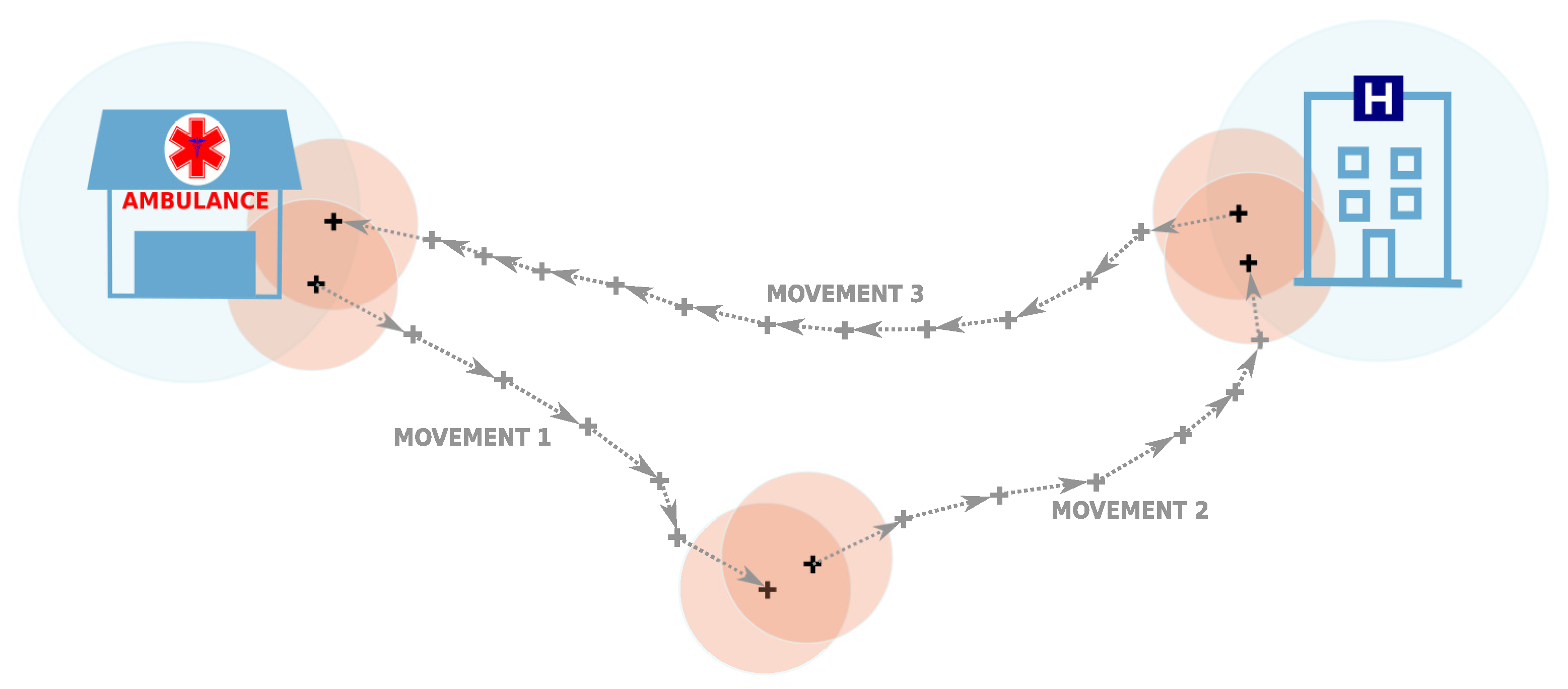
- Formation of ambulance trips: We define a trip of an ambulance as a sequence of co-located movements, and this sequence is initiated and terminated at an ambulance station, where is a subsequence of indices such that i is a member of this subsequence if and only if the aerial distance between the points and p is not larger than 300 m. (We remark that p is a position of ambulance station and is an appropriate natural number.) Two consecutive movements and are considered to be co-located if the aerial distance between the terminal point of the first movement and the initial point of the second movement is less than 200 m and the time difference is not larger than 2 h. Initial and terminal points of a movement were associated with an ambulance station or hospital if the aerial distance between them was less than or equal to 300 m (for an illustration, see Figure 3). GPS positions of ambulance stations and hospitals that are deployed across the Slovak Republic were kindly provided to us by the authors of the work [46]. Trips were assembled by processing the created movements (movement by movement) in the order of timestamps associated with the initial GPS measurements. The process of building an ambulance trip was initiated when the first GPS measurement of the movement was associated with an ambulance station. A trip was grown by appending co-located movements until a movement was found with the terminal point associated with the initial emergency station. Hence, a trip was a closed-loop initiated and terminated at the position of an ambulance station. If a pair of movements that were not collocated was encountered while an ambulance trip was being formed, the forming process was cancelled, and the next movement with the first GPS point associated with an ambulance station was used to initiate the process of trip building. The formation process continued until all movements were processed.
- Amendment of ambulance trips: By evaluating a sample set of ambulance trips visualised on the map, we concluded that the majority of extracted trips were proper and ready for analysis. However, some flaws that repeated multiple times were identified:
- –
- Some trips contained very short movements, which appeared to be insignificant. Often, it was initial or terminal movement located within the area of an ambulance station.
- –
- Some trips approached a hospital or an ambulance station, but the movement was not split into two movements (i.e., the potential stop was not recognised).
- –
- Some trips were very short in length and in time.
- –
- Some trips were very long and very complex to interpret (taking a long time and having many stops till the ambulance returned back to the initial ambulance station).
To mitigate these problems, additional procedures were implemented:- –
- Pruning of initial and terminal movements: When the initial and terminal movements of a trip were very short and took place within the close surroundings of an ambulance station, they were insignificant for the trip. Therefore, a sequence of initial (terminal) movements was eliminated from the trip if their terminal (initial) point was closer than 300 metres from the ambulance station.
- –
- Merging of insignificant inner movements: In further analyses, we considered inner movements of a trip only in the context of hospitals, ambulance stations, and potential locations of patients that could be associated with the initial and terminal points of inner movements. Therefore, short inner movements (no longer than 500 m) were merged with the preceding or the following movements belonging to the same trip if either the endpoint of both movements was associated with the same ambulance station (and/or hospital) or both endpoints were not associated with any known point of interest (ambulance station or hospital).
- –
- The addition of potentially relevant stops: To not miss a potentially relevant stop of an ambulance at an ambulance station or a hospital, all movements were scanned by inspecting all inner GPS measurements. If an inner GPS measurement with the instantaneous velocity equal to zero was detected, it was checked whether it could have been associated (i.e., it was located closer than 300 m) with an ambulance station or hospital different from the ambulance station(s) or hospital(s) the initial and terminal points of a given movement were associated with. If there was more than one such inner point, the inner point which was closest to a given ambulance station or hospital was found. The movement was cut at an identified inner point, and two movements were formed.
- Filtering of emergency ambulance trips: Finally, to obtain an interpretable set of trips, we applied a set of simple filters. Trips composed of two movements were always selected. Trips consisting of more than two movements were selected only if at least 50% of initial and terminal points of inner movements were associated either with a hospital or with an ambulance station. To prevent the selection of trips that were too short or too complex for further analysis, we evaluated the overall lengths and durations of trips. We only selected trips longer than 1 km (to exclude short technical trips typically done within the area of an ambulance station) and shorter than 500 km (the distance that should be sufficient to accommodate trips to major Slovak hospitals located in the cities of Bratislava and Košice). For similar reasons, we considered only trips taking more than 15 min and less than six h.
4. Results
4.1. Extraction of Emergency Ambulance Trips
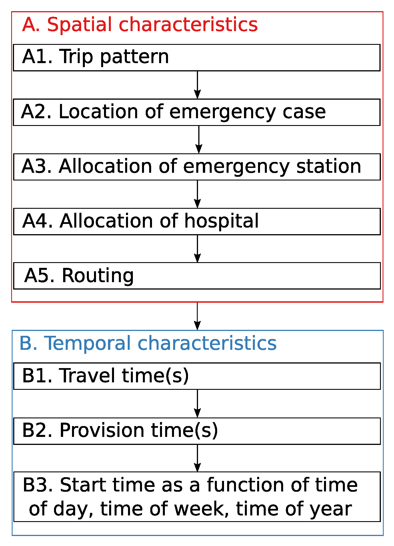
4.2. Modelling of Ambulance Trips
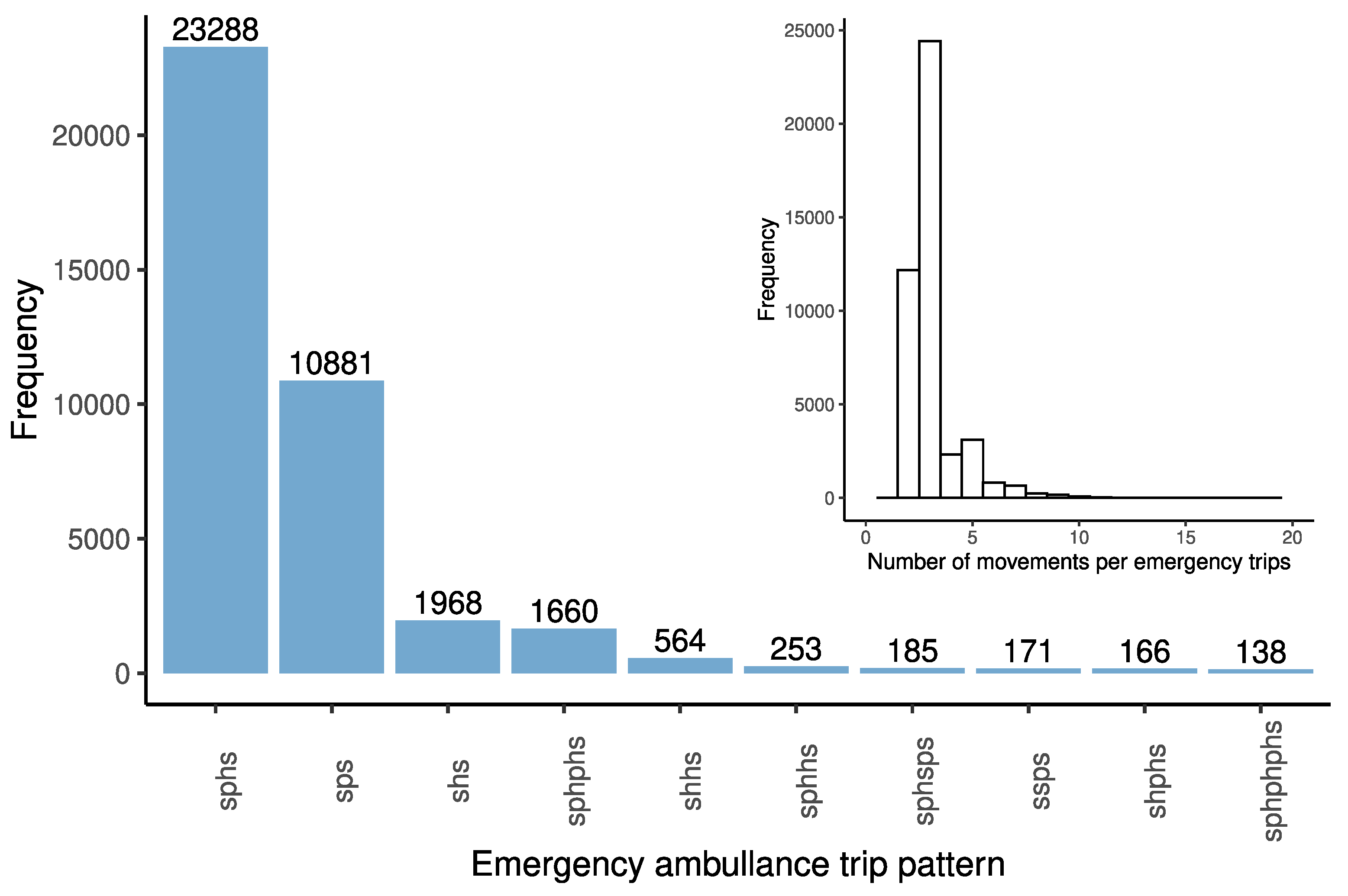
4.2.1. Trip Patterns
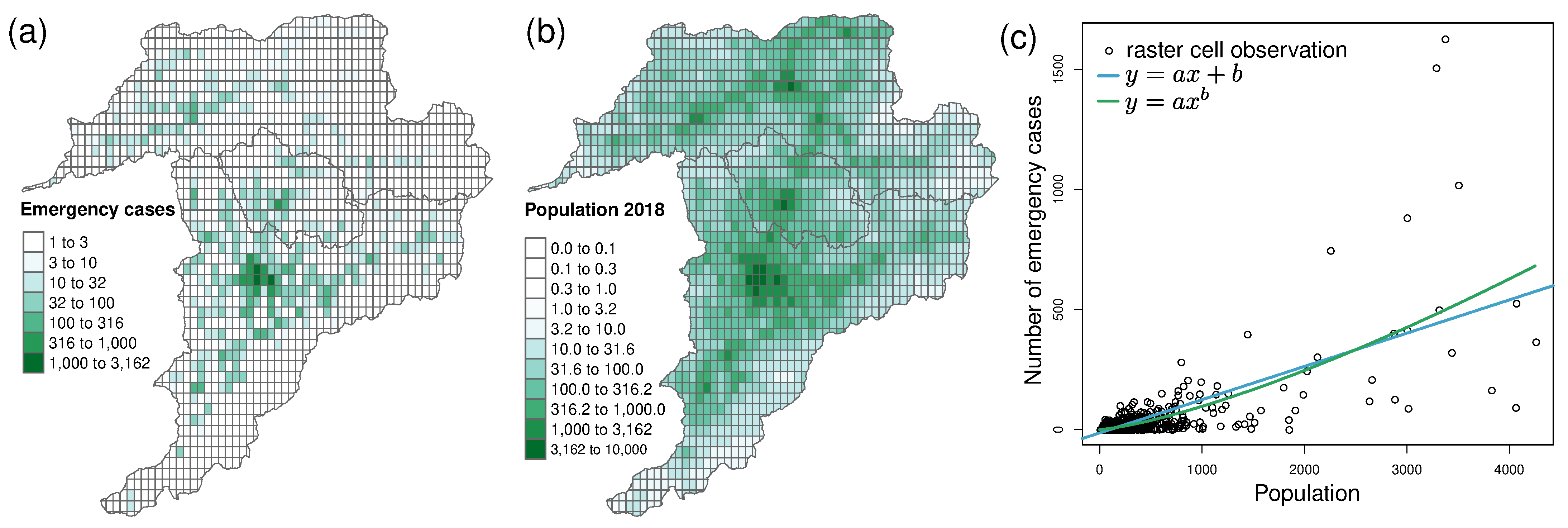
4.2.2. Locations of Emergency Cases
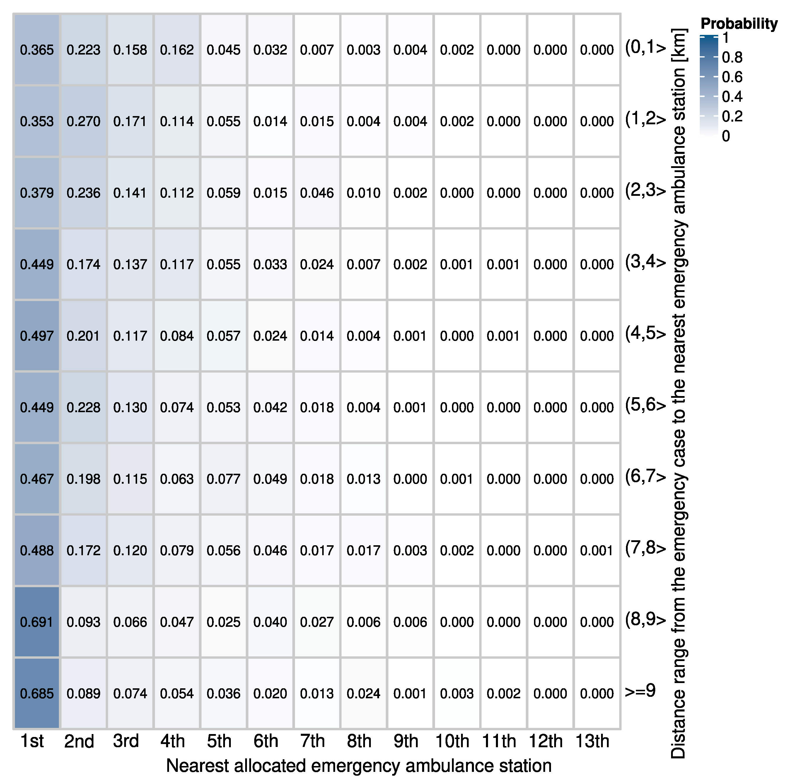
4.2.3. Allocation of Emergency Cases to Stations and Hospitals
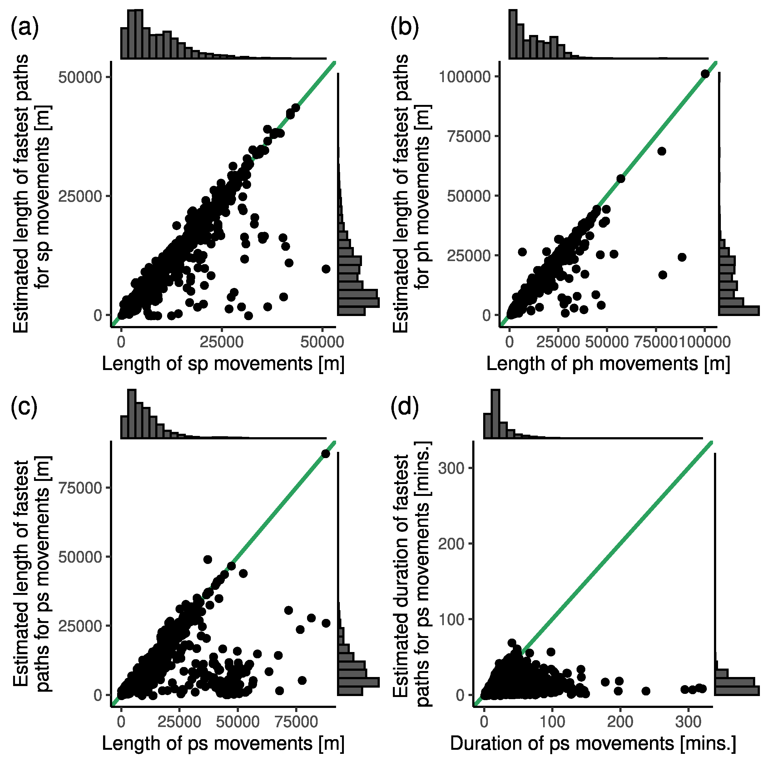
4.2.4. Routing of Emergency Ambulances
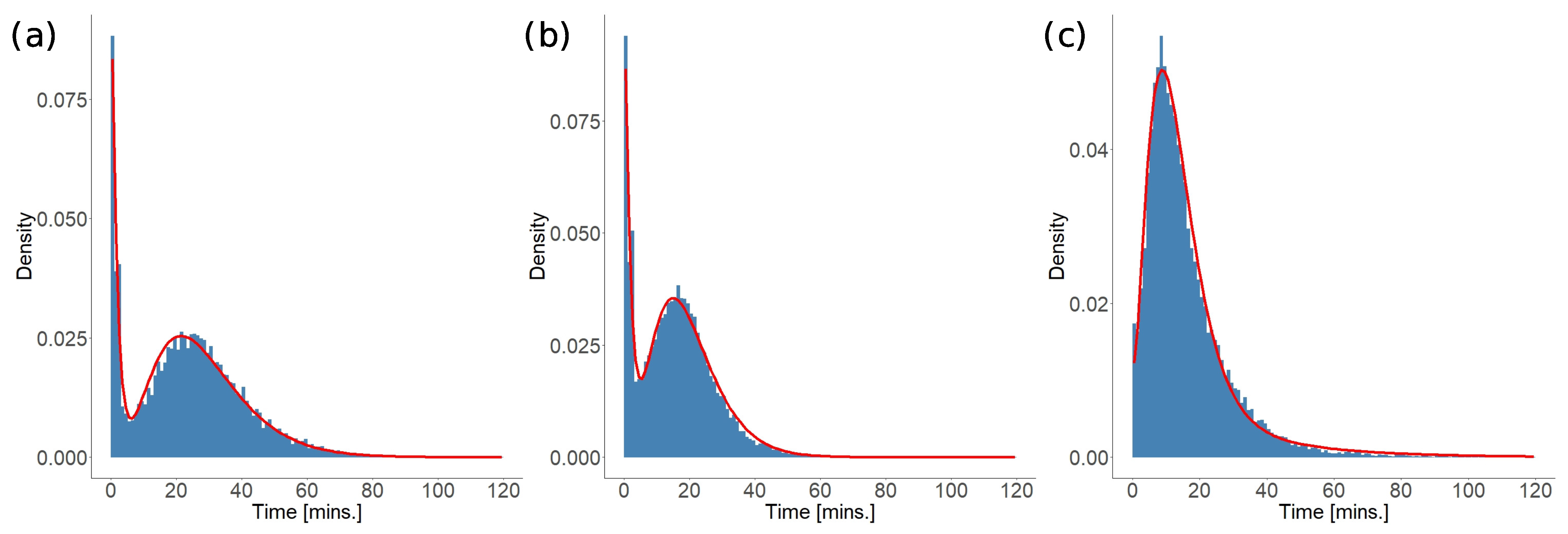
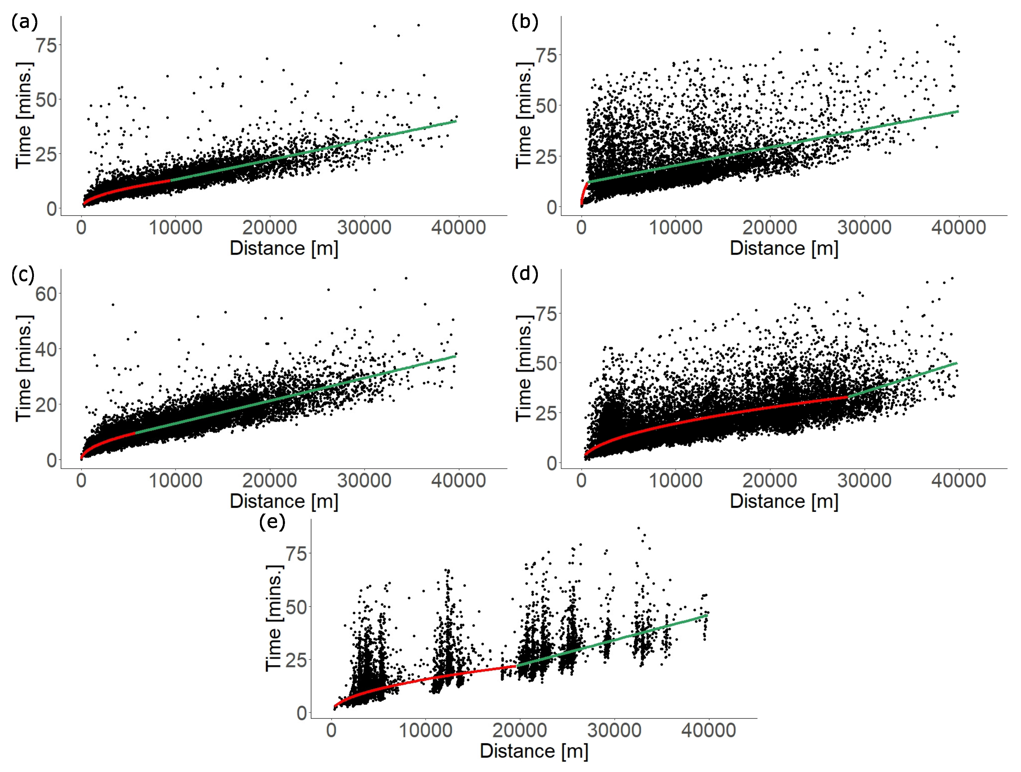
4.2.5. Travel Time
4.2.6. Provision Times
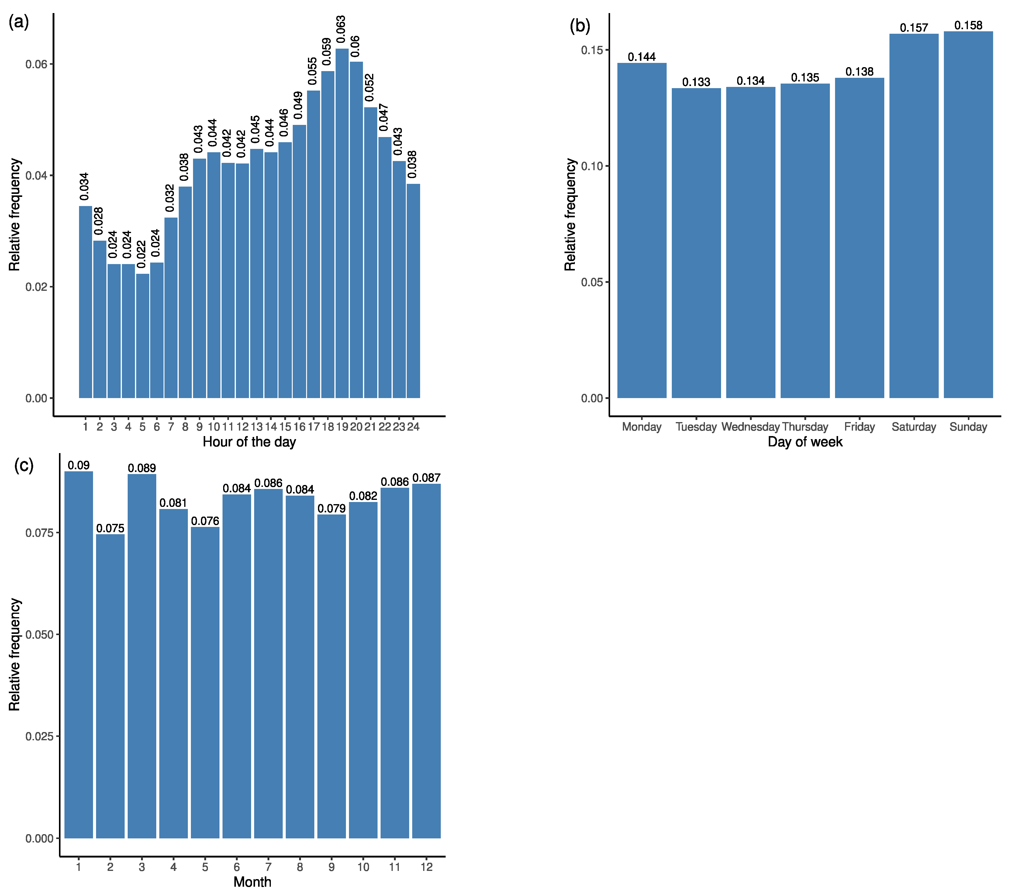
4.2.7. Modelling the Start Times of Ambulance Trips
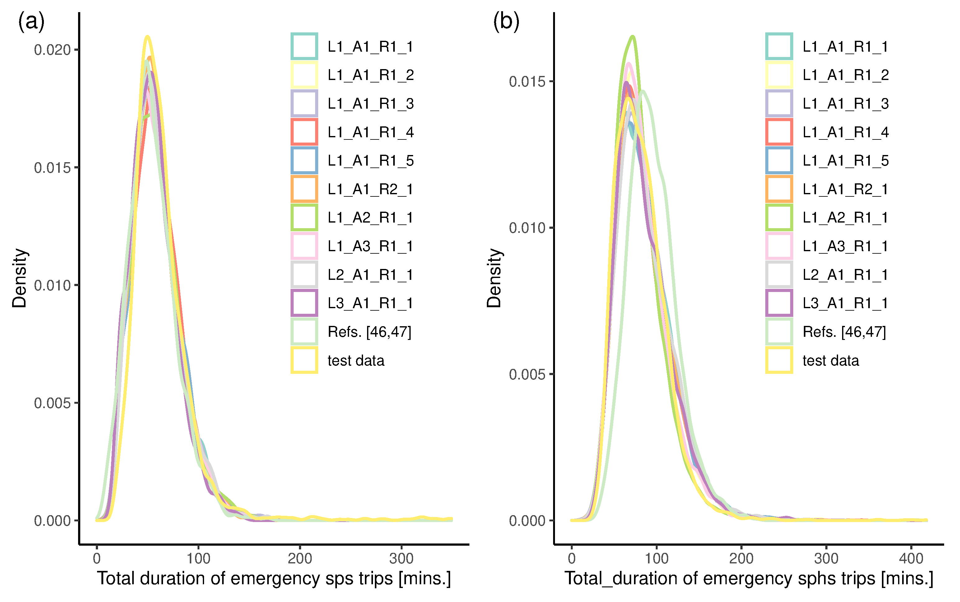
4.3. Validation of Models
- Location of an emergency case (see Section 4.2.2):
- —default: By exponential model to identify a grid cell and then choose a location within a cell with uniform probability.
- —alternative: By the linear model to choose a grid cell and then find a location within a cell with uniform probability.
- —alternative: To choose a grid cell with empirical probabilities (derived from data) and then find a location within a cell with uniform probability. Comparison of this option with and enables us to evaluate the models locating the emergency cases based on the proposed models that depend on the population density.
- Allocation of an emergency case (see Section 4.2.3):
- –default: To a hospital following the empirical probabilities of allocating a station to the 1st, 2nd, 3rd, and so on closest hospital;
- —alternative: To the closest hospital;
- —alternative: To a hospital following the closest-hospital-specific empirical probability distribution to allocate a station to the 1st, 2nd, 3rd, and so on closest hospital.
- Routing (see Section 4.2.4):
- —default: Following the fastest path in the road network;
- —alternative: Following the shortest path in the road network.
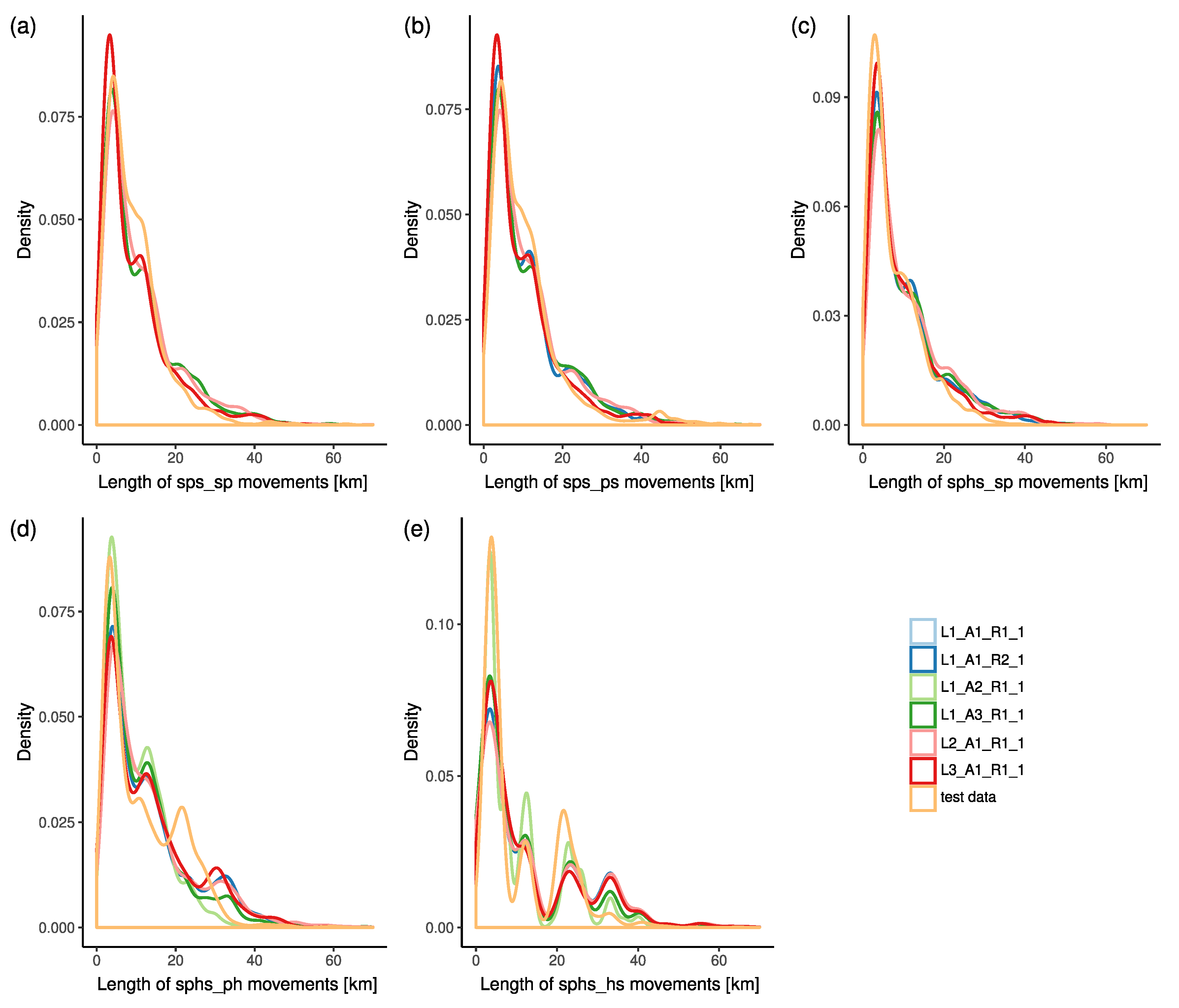
4.3.1. Validation of Spatial Characteristics
4.3.2. Validation of Temporal Characteristics
4.4. Use of the Data Models in Simulations and Optimisations
5. Conclusions
Limitations and Future Research
Supplementary Materials
Author Contributions
Funding
Institutional Review Board Statement
Informed Consent Statement
Data Availability Statement
Acknowledgments
Conflicts of Interest
Abbreviations
| EMS | Emergency Medical Services |
| GPS | Global Positioning System |
| API | Application Programming Interface |
| GSM | Global System for Mobile Communications |
| sps | station-patient-station drive |
| sphs | station-patient-hospital-station drive |
| MAPE | Mean Percentage Absolute Error |
| RMSE | Root Mean Square Error |
| KS | Kolmogorov–Smirnov |
| KL | Kullback–Leibler |
References
- Zaffar, M.A.; Rajagopalan, H.K.; Saydam, C.; Mayorga, M.; Sharer, E. Coverage, survivability or response time: A comparative study of performance statistics used in ambulance location models via simulation–optimization. Oper. Res. Health Care 2016, 11, 1–12. [Google Scholar] [CrossRef]
- Erkut, E.; Ingolfsson, A.; Erdogan, G. Ambulance location for maximum survival. Nav. Res. Logist. 2008, 55, 42–58. [Google Scholar] [CrossRef]
- Zhang, Z.; He, Q.; Gou, J.; Li, X. Analyzing travel time reliability and its influential factors of emergency vehicles with generalized extreme value theory. J. Intell. Transp. Syst. Technol. Plan. Oper. 2019, 23, 1–11. [Google Scholar] [CrossRef]
- Eiselt, H.A.; Marianov, V. Foundations of Location Analysis; Business and Economics ed.; Springer: Boston, MA, USA, 2012. [Google Scholar]
- Eiselt, H.A.; Marianov, V. Applications of Location Analysis; Business and Economics ed.; Springer: Boston, MA, USA, 2015; Volume 232. [Google Scholar] [CrossRef]
- Brotcorne, L.; Laporte, G.; Semet, F. Ambulance location and relocation models. Eur. J. Oper. Res. 2003, 147, 451–463. [Google Scholar] [CrossRef]
- Farahani, R.Z.; Asgari, N.; Heidari, N.; Hosseininia, M.; Goh, M. Covering problems in facility location: A review. Comput. Ind. Eng. 2012, 62, 368–407. [Google Scholar] [CrossRef]
- Farahani, R.Z.; SteadieSeifi, M.; Asgari, N. Multiple criteria facility location problems: A survey. Appl. Math. Model. 2012, 34, 1689–1709. [Google Scholar] [CrossRef]
- Basar, A.; Catay, B.; Unluyurt, T. A taxonomy for emergency service station location problem. Optim. Lett. 2012, 6, 1147–1160. [Google Scholar] [CrossRef] [Green Version]
- Marianov, V. Location Models for Emergency Service Applications. 2017. Chapter 11. pp. 237–262. Available online: https://pubsonline.informs.org/doi/abs/10.1287/educ.2017.0172 (accessed on 14 September 2020).
- Aringhieri, R.; Bruni, M.; Khodaparasti, S.; van Essen, J. Emergency medical services and beyond: Addressing new challenges through a wide literature review. Comput. Oper. Res. 2017, 78, 349–368. [Google Scholar] [CrossRef]
- Yao, J.; Zhang, X.; Murray, A.T. Location optimization of urban fire stations: Access and service coverage. Comput. Environ. Urban Syst. 2019, 73, 184–190. [Google Scholar] [CrossRef]
- Degel, D.; Wiesche, L.; Rachuba, S.; Werners, B. Reorganizing an existing volunteer fire station network in Germany. Socio-Econ. Plan. Sci. 2014, 48, 149–157. [Google Scholar] [CrossRef]
- Cudnik, M.T.; Yao, J.; Zive, D.; Newgard, C.; Murray, A.T. Surrogate markers of transport distance for out-of-hospital cardiac arrest patients. Prehosp. Emerg. Care 2012, 16, 266–272. [Google Scholar] [CrossRef]
- Murray, A.T. Optimising the spatial location of urban fire stations. Fire Saf. J. 2013, 62, 64–71. [Google Scholar] [CrossRef]
- Murray, A.T. Fire Station Siting; Springer International Publishing: Cham, Switzerland, 2015; pp. 293–306. [Google Scholar]
- Jia, T.; Tao, H.; Qin, K.; Wang, Y.; Liu, C.; Gao, Q. Selecting the optimal healthcare centers with a modified p-median model: A visual analytic perspective. Int. J. Health Geogr. 2014, 13, 42. [Google Scholar] [CrossRef] [PubMed] [Green Version]
- Cebecauer, M.; Buzna, Ľ. A versatile adaptive aggregation framework for spatially large discrete location-allocation problems. Comput. Ind. Eng. 2017, 111, 364–380. [Google Scholar] [CrossRef]
- Ingolfsson, A.; Budge, S.; Erkut, E. Optimal ambulance location with random delays and travel times. Health Care Manag. Sci. 2008, 11, 262–274. [Google Scholar] [CrossRef]
- Gu, W.; Wang, X.; McGregor, S.E. Optimization of preventive health care facility locations. Int. J. Health Geogr. 2010, 18, 9–17. [Google Scholar] [CrossRef] [Green Version]
- Knight, V.; Harper, P.; Smith, L. Ambulance allocation for maximal survival with heterogeneous outcome measures. Omega 2012, 40, 918–926. [Google Scholar] [CrossRef]
- Van Barneveld, T.C.; Bhulai, S.; van der Mei, R.D. A dynamic ambulance management model for rural areas. Health Care Manag. Sci. 2017, 20, 165–186. [Google Scholar] [CrossRef]
- McLay, L.A.; Mayorga, M.E. Evaluating emergency medical service performance measures. Health Care Manag. Sci. 2010, 13, 124–136. [Google Scholar] [CrossRef]
- Jagtenberg, C.J.; Bhulai, S.; van der Mei, R.D. Dynamic ambulance dispatching: Is the closest-idle policy always optimal? Health Care Manag. Sci. 2017, 20, 517–531. [Google Scholar] [CrossRef] [PubMed] [Green Version]
- Lam, S.S.W.; Zhang, Z.C.; Oh, H.C.; Ng, Y.Y.; Wah, W.; Ong, M.E.H. Reducing ambulance response times using discrete event simulation. Prehosp. Emerg. Care 2014, 18, 207–216. [Google Scholar] [CrossRef]
- Nogueira, L.C.; Pinto, L.R.; Silva, P.M.S. Reducing emergency medical service response time via the reallocation of ambulance bases. Health Care Manag. Sci. 2016, 19, 31–42. [Google Scholar] [CrossRef] [PubMed]
- Fisher, R.; Lassa, J. Interactive, open source, travel time scenario modelling: Tools to facilitate participation in health service access analysis. Int. J. Health Geogr. 2017, 16. [Google Scholar] [CrossRef] [PubMed] [Green Version]
- Erkut, E.; Fenske, R.; Kabanuk, S.; Gardiner, Q.; Davis, J. Improving the emergency service delivery in St. Albert. INFOR Inf. Syst. Oper. Res. 2001, 39, 416–433. [Google Scholar] [CrossRef]
- Budge, S.; Ingolfsson, A.; Zerom, D. Empirical analysis of ambulance travel times: The case of Calgary emergency medical services. Manag. Sci. 2010, 56, 716–723. [Google Scholar] [CrossRef]
- McLay, L.A.; Boone, E.L.; Brooks, J.P. Analyzing the volume and nature of emergency medical calls during severe weather events using regression methodologies. Socio-Econ. Plan. Sci. 2012, 46, 55–66. [Google Scholar] [CrossRef]
- Earnest, A.; Ong, M.E.H.; Shahidah, N.; Ng, W.M.; Foo, C.; Nott, D.J. Spatial analysis of ambulance response times related to prehospital cardiac arrests in the city-state of Singapore. Prehosp. Emerg. Care 2012, 16, 256–265. [Google Scholar] [CrossRef]
- Seim, J.; Glenn, M.J.; English, J.; Sporer, K. Neighborhood poverty and 9-1-1 ambulance response time. Prehosp. Emerg. Care 2018, 22, 436–444. [Google Scholar] [CrossRef] [Green Version]
- Fleischman, R.J.; Lundquist, M.; Jui, J.; Newgard, C.D.; Warden, C. Predicting ambulance time of arrival to the emergency department using global positioning system and google maps. Prehospital Emerg. Care 2013, 17, 458–465. [Google Scholar] [CrossRef] [Green Version]
- Degel, D.; Wiesche, L.; Rachuba, S.; Werners, B. Time-dependent ambulance allocation considering data-driven empirically required coverage. Health Care Manag. Sci. 2015, 18, 444–458. [Google Scholar] [CrossRef]
- Sasaki, S.; Comber, A.J.; Suzuki, H.; Brunsdon, C. Using genetic algorithms to optimise current and future health planning - the example of ambulance locations. Int. J. Health Geogr. 2010, 9. [Google Scholar] [CrossRef] [PubMed] [Green Version]
- Grekousis, G.; Liu, Y. Where will the next emergency event occur? predicting ambulance demand in emergency medical services using artificial intelligence. Comput. Environ. Urban Syst. 2019, 76, 110–122. [Google Scholar] [CrossRef]
- Derekenaris, G.; Garofalakis, J.; Makris, C.; Prentzas, J.; Sioutas, S.; Tsakalidis, A. Integrating gis, gps and gsm technologies for the effective management of ambulances. Comput. Environ. Urban Syst. 2001, 25, 267–278. [Google Scholar] [CrossRef]
- Phan, A.; Ferrie, F.P. Interpolating sparse gps measurements via relaxation labeling and belief propagation for the redeployment of ambulances. IEEE Trans. Intell. Transp. Syst. 2011, 12, 1587–1598. [Google Scholar] [CrossRef]
- Poulton, M.; Noulas, A.; Weston, D.; Roussos, G. Modeling metropolitan-area ambulance mobility under blue light conditions. IEEE Access 2019, 7, 1390–1403. [Google Scholar] [CrossRef]
- Westgate, B.S.; Woodard, D.B.; Matteson, D.S.; Henderson, S.G. Travel time estimation for ambulances using Bayesian data augmentation. Ann. Appl. Stat. 2013, 7, 1139–1161. [Google Scholar] [CrossRef] [Green Version]
- Westgate, B.S.; Woodard, D.B.; Matteson, D.S.; Henderson, S.G. Large-network travel time distribution estimation for ambulances. Eur. J. Oper. Res. 2016, 252, 322–333. [Google Scholar] [CrossRef]
- Piorkowski, A. Construction of a dynamic arrival time coverage map for emergency medical services. Open Geosci. 2018, 10, 67–173. [Google Scholar] [CrossRef]
- Van Dijk, J. Identifying activity-travel points from GPS-data with multiple moving windows. Comput. Environ. Urban Syst. 2018, 70, 84–101. [Google Scholar] [CrossRef]
- Koháni, M.; Czimmermann, P.; Váňa, M.; Cebecauer, M.; Buzna, Ľ. Location-scheduling optimization problem to design private charging infrastructure for electric vehicles. In Operations Research and Enterprise Systems; Revised Selected Papers; Communications in Computer and Information Science; Springer: Berlin/Heidelberg, Germany, 2017. [Google Scholar]
- Kolesar, P.; Walker, W.; Hausner, J. Determining the relation between fire engine travel times and travel distances in New York City. Oper. Res. 1975, 23, 614–627. [Google Scholar] [CrossRef] [Green Version]
- Jánošíková, Ľ.; Kvet, M.; Jankovič, P.; Gábrišová, L. An optimization and simulation approach to emergency stations relocation. Cent. Eur. J. Oper. Res. 2019, 27, 737–758. [Google Scholar] [CrossRef]
- Jánošíková, Ľ.; Jankovič, P.; Kvet, M.; Zajacová, F. Coverage versus response time objectives in ambulance location. Int. J. Health Geogr. 2021, 20, 32. [Google Scholar] [CrossRef] [PubMed]
- Janáček, J.; Jánošíková, Ľ.; Buzna, Ľ. Optimized design of large-scale social welfare supporting systems oncomplex networks. In Optimization in Complex Networks: Theory and Applications; Springer Science + Business Media: New York, NY, USA, 2012; pp. 337–361. ISBN 978-1-4614-0753-9. e-ISBN 978-1-4614-0754-6. [Google Scholar]
- WorldPop, “Gridded Residential Population Data”. 2020. Available online: https://www.worldpop.org (accessed on 14 September 2020).
- Oak Ridge National Laboratory. Landscan Dataset. 2020. Available online: https://landscan.ornl.gov/landscan-datasets (accessed on 14 September 2020).
- HERE Platform. Landscan Dataset. 2021. Available online: https://developer.here.com/ (accessed on 25 February 2021).
- Chatterjee, S.; Hadi, A.S. Regression Analysis by Example; John Wiley & Sons: Hoboken, NJ, USA, 2015. [Google Scholar]
- James, G.; Witten, D.; Hastie, T.; Tibshirani, R. An Introduction to Statistical Learning; Springer: Berlin/Heidelberg, Germany, 2013; Volume 112. [Google Scholar]
- Goodfellow, I.; Bengio, Y.; Courville, A. Deep Learning; MIT Press: Cambridge, MA, USA, 2016. [Google Scholar]


| Raster Cell Size [m × m] | Model | a | b | adj. |
|---|---|---|---|---|
| 0.145 | −0.198 | 0.253 | ||
| 0.080 | 1.103 | 0.254 | ||
| 0.138 | −5.751 | 0.412 | ||
| 0.019 | 1.278 | 0.423 | ||
| 0.139 | −14.539 | 0.468 | ||
| 0.009 | 1.351 | 0.488 | ||
| 0.136 | −23.532 | 0.595 | ||
| 0.006 | 1.369 | 0.625 |
| Movement Type | Real Paths | ||||||
|---|---|---|---|---|---|---|---|
| Length [m] | Duration [min.] | ||||||
| MAPE | RMSE | Pearson | MAPE | RMSE | Pearson | ||
| Shortest paths | sp | 0.079 | 2222.6 | 0.948 | 0.280 | 12.2 | 0.432 |
| ph | 0.136 | 2656.9 | 0.962 | 0.323 | 11.6 | 0.604 | |
| hs | 0.105 | 1492.4 | 0.988 | 0.322 | 12.6 | 0.570 | |
| ps | 0.168 | 6860.1 | 0.678 | 0.342 | 22.7 | 0.180 | |
| Fastest paths | sp | 0.071 | 2085.2 | 0.952 | 0.257 | 11.9 | 0.439 |
| ph | 0.135 | 2491.5 | 0.965 | 0.294 | 11.5 | 0.610 | |
| hs | 0.151 | 1562.0 | 0.986 | 0.288 | 12.4 | 0.676 | |
| ps | 0.165 | 6794.1 | 0.680 | 0.335 | 22.7 | 0.178 | |
| Movement Type | Model Parameters | |||
|---|---|---|---|---|
| sps_sp | 9471 | |||
| sps_ps | 678 | |||
| sphs_sp | 5745 | |||
| sphs_ph | 28,239 | |||
| sphs_hs | 19,554 | |||
| Trip Type (Stop) | Model Parameters | ||||
|---|---|---|---|---|---|
| sps (p) | 0.19 | 0.59 | 1 | 0.14 | 4 |
| sphs (p) | 0.21 | 0.54 | 1 | 0.2 | 4 |
| sphs (h) | 0.29 | 0.04 | 1 | 0.22 | 3 |
| K-S Test Values | Trip Type (Stop) | ||
|---|---|---|---|
| sps (p) | sphs (p) | sphs (h) | |
| 0.137 | 0.136 | 0.136 | |
| D | 0.077 | 0.089 | 0.091 |
| Trip Pattern | Total Number of Trips | Average Number of Trips/Month |
|---|---|---|
| sps | 10,881 | 294.1 |
| sphs | 23,288 | 629.4 |
| Model | Movement | |||||
|---|---|---|---|---|---|---|
| sps_sp | sps_ps | sphs_sp | sphs_ph | sphs_hs | ||
| L1_A1_R1_1 | 0.014 | 0.014 | 0.023 | 0.042 | 0.112 | 0.041 |
| L1_A1_R1_2 | 0.013 | 0.014 | 0.021 | 0.038 | 0.109 | 0.039 |
| L1_A1_R1_3 | 0.019 | 0.017 | 0.028 | 0.041 | 0.129 | 0.047 |
| L1_A1_R1_4 | 0.019 | 0.020 | 0.025 | 0.039 | 0.111 | 0.043 |
| L1_A1_R1_5 | 0.016 | 0.016 | 0.022 | 0.038 | 0.120 | 0.042 |
| L1_A1_R2 | 0.014 | 0.016 | 0.016 | 0.039 | 0.103 | 0.038 |
| L1_A2_R1 | 0.014 | 0.014 | 0.022 | 0.032 | 0.043 | 0.025 |
| L1_A3_R1 | 0.014 | 0.014 | 0.022 | 0.031 | 0.071 | 0.030 |
| L2_A1_R1 | 0.007 | 0.007 | 0.035 | 0.053 | 0.116 | 0.044 |
| L3_A1_R1 | 0.025 | 0.028 | 0.009 | 0.031 | 0.081 | 0.035 |
| Model | Movement | Trip | ||||||
|---|---|---|---|---|---|---|---|---|
| sps_sp | sps_ps | sphs_sp | sphs_ph | sphs_hs | sps | sphs | ||
| L1_A1_R1_1 | 0.012 | 0.075 | 0.026 | 0.039 | 0.178 | 0.066 | 0.013 | 0.006 |
| L1_A1_R1_2 | 0.010 | 0.075 | 0.024 | 0.036 | 0.180 | 0.065 | 0.019 | 0.007 |
| L1_A1_R1_3 | 0.014 | 0.071 | 0.028 | 0.038 | 0.212 | 0.073 | 0.016 | 0.007 |
| L1_A1_R1_4 | 0.015 | 0.065 | 0.030 | 0.041 | 0.184 | 0.067 | 0.014 | 0.006 |
| L1_A1_R1_5 | 0.012 | 0.072 | 0.026 | 0.039 | 0.187 | 0.067 | 0.010 | 0.005 |
| L1_A1_R2 | 0.012 | 0.072 | 0.022 | 0.037 | 0.156 | 0.060 | 0.018 | 0.008 |
| L1_A2_R1 | 0.012 | 0.066 | 0.025 | 0.058 | 0.229 | 0.078 | 0.017 | 0.004 |
| L1_A3_R1 | 0.012 | 0.066 | 0.025 | 0.043 | 0.153 | 0.060 | 0.011 | 0.006 |
| L2_A1_R1 | 0.007 | 0.072 | 0.034 | 0.044 | 0.174 | 0.066 | 0.012 | 0.010 |
| L3_A1_R1 | 0.020 | 0.072 | 0.017 | 0.030 | 0.092 | 0.046 | 0.022 | 0.006 |
Publisher’s Note: MDPI stays neutral with regard to jurisdictional claims in published maps and institutional affiliations. |
© 2021 by the authors. Licensee MDPI, Basel, Switzerland. This article is an open access article distributed under the terms and conditions of the Creative Commons Attribution (CC BY) license (https://creativecommons.org/licenses/by/4.0/).
Share and Cite
Buzna, Ľ.; Czimmermann, P. On the Modelling of Emergency Ambulance Trips: The Case of the Žilina Region in Slovakia. Mathematics 2021, 9, 2165. https://doi.org/10.3390/math9172165
Buzna Ľ, Czimmermann P. On the Modelling of Emergency Ambulance Trips: The Case of the Žilina Region in Slovakia. Mathematics. 2021; 9(17):2165. https://doi.org/10.3390/math9172165
Chicago/Turabian StyleBuzna, Ľuboš, and Peter Czimmermann. 2021. "On the Modelling of Emergency Ambulance Trips: The Case of the Žilina Region in Slovakia" Mathematics 9, no. 17: 2165. https://doi.org/10.3390/math9172165
APA StyleBuzna, Ľ., & Czimmermann, P. (2021). On the Modelling of Emergency Ambulance Trips: The Case of the Žilina Region in Slovakia. Mathematics, 9(17), 2165. https://doi.org/10.3390/math9172165