Matrix Profile-Based Approach to Industrial Sensor Data Analysis Inside RDBMS

Abstract

Currently, big sensor data arise in a wide spectrum of Industry 4.0, Internet of Things, and Smart City applications. In such subject domains, sensors tend to have a high frequency and produce massive time series in a relatively short time interval. The data collected from the sensors are subject to mining in order to make strategic decisions. In the article, we consider the problem of choosing a Time Series Database Management System (TSDBMS) to provide efficient storing and mining of big sensor data. We overview InfluxDB, OpenTSDB, and TimescaleDB, which are among the most popular state-of-the-art TSDBMSs, and represent different categories of such systems, namely native, add-ons over NoSQL systems, and add-ons over relational DBMSs (RDBMSs), respectively. Our overview shows that, at present, TSDBMSs offer a modest built-in toolset to mine big sensor data. This leads to the use of third-party mining systems and unwanted overhead costs due to exporting data outside a TSDBMS, data conversion, and so on. We propose an approach to managing and mining sensor data inside RDBMSs that exploits the Matrix Profile concept. A Matrix Profile is a data structure that annotates a time series through the index of and the distance to the nearest neighbor of each subsequence of the time series and serves as a basis to discover motifs, anomalies, and other time-series data mining primitives. This approach is implemented as a PostgreSQL extension that allows an application programmer both to compute matrix profiles and mining primitives and to represent them as relational tables. Experimental case studies show that our approach surpasses the above-mentioned out-of-TSDBMS competitors in terms of performance since it assumes that sensor data are mined inside a TSDBMS at no significant overhead costs.

1. Introduction

Currently, big sensor data arise in a wide spectrum of  Industry 4.0 [1], Internet of Things (IoT) [2], Smart City [3], and Smart Home [4] applications. In such subject domains, sensors tend to have high frequency (for example, tens of times per second) and produce time series of tens of millions to billions of elements in a relatively short time interval. The data obtained from sensors should be stored permanently and subjected to mining to extract hidden knowledge and make strategic decisions. In performing these tasks, a Time Series Database Management System (TSDBMS) plays a critically important role to provide an application programmer with means and tools to efficiently process and analyze such amounts of sensor data.

In this article, we consider the problem of choosing an appropriate TSDBMS for managing and mining big sensor data. TSDBMSs differ from both relational DBMSs (RDBMSs) and NoSQL systems. A TSDBMS does not need a transaction mechanism since sensor data are collected but not deleted or modified. Also, a TSDBMS should provide efficient operations for adding new atomic values that arrive in streaming mode, yet efficient mining operations where a time series is considered as a whole.

At present, despite the widespread use of NoSQL systems, RDBMSs remain the basic work tools to store and manipulate data in a wide spectrum of subject domains. This claim is supported by the statistics of the DB-Engines.com portal

(see DBMS popularity broken down by database model, https://db-engines.com/en/ranking_categories, accessed on 12 April 2021) pointing out that relational DBMSs hold up to 75 percent of the market. By its nature, an RDBMS does not provide built-in data mining functions, whereas the development of in-RDBMS data mining methods is a topical issue [5]. Indeed, if we consider an RDBMS only as a data repository, this may lead to significant overheads when exporting large data volumes outside the RDBMS, changing data format, and importing the results of the analysis back to RDBMS. In-RDBMS data mining methods cover SQL-based implementations of various problems (for example, association rules [6,7], clustering [8,9], graph mining [10,11], and others) as well as multipurpose libraries and frameworks [12,13,14,15]. However, to the best of our knowledge, there are no developments related to in-RDBMS time-series mining.

The article contributes as follows. We present an approach to managing and mining sensor data inside RDBMS, based on the Matrix Profile concept. Matrix Profile [16] is a data structure that annotates a time series through the index of and the distance to the nearest neighbor of each subsequence of the series. Sensor data and Matrix Profile structures that support the mining are represented as relational tables. Sensor data are mined inside an RDBMS at no significant overhead costs for export-import data. We implemented this approach as a PostgreSQL extension. Our experiments on real cases show that our approach surpasses out-of-TSDBMS competitors in terms of performance.

The rest of the article is organized as follows. Section 2 provides a brief overview of the most popular state-of-the-art TSDBMSs. Section 3 presents an approach to managing and mining sensor data inside RDBMS. Section 4 describes the experimental evaluation of our approach. Section 5 contain a summary of the results obtained and directions for further research.

2. Overview of Modern Time Series DBMSs

2.1. Classification of Time Series DBMSs

In [17], the authors employ the following four-group classification of TSDBMSs. The first group includes systems that provide time series storage based on a third-party RDBMS or NoSQL system. The systems of the second group provide time series storage independently. The third group consists of RDBMSs providing tools to store and process time series. Finally, the fourth group is represented by commercial systems regardless of their basic data model, an underlying third-party RDBMS or NoSQL system to store time series, etc.

In this article, we distinguish native and add-on TSDBMSs. A native TSDBMS is a stand-alone proprietary or free development with an original query language, database engine, data storage system, and so forth. There is a wide spectrum of native systems: InfluxDB [18], Prometheus [17], Druid [19], LittleTable [20], FluteDB [21], PhilDB [22], EdgeDB [23], TSMMDB [24], and others.

An add-on TSDBMS is implemented on top of a third-party system that provides the TSDBMS with a database engine and a data storage system. Depending on the data model exploited by the basic system, one can distinguish between an add-on TSDBMS over a NoSQL system or an RDBMS.

Currently, a wide range of add-on TSDBMSs is built on top of the following NoSQL systems. The  OpenTSDB [17] and Gorilla [25] add-on systems run over HBase [26]. BTrDB [27] is deployed on a distributed file systems, namely HDFS [28], GlusterFS [29], or CephFS [29]. Also, BTrDB can exploit one of the NoSQL systems as a database engine, namely MongoDB [30], Cassandra, or HBase [26]. KairosDB [17] is based on Cassandra [26]. The tsdb [31] system works in conjunction with the Berkeley DB [32] embedded DBMS. HeteroTSDB [33] runs over the Amazon DynamoDB [34] system.

The subclass of add-on TSDBMSs based on relational DBMSs is pretty small; its basic representatives are TimescaleDB [18] built over PostgreSQL [35], and RecovDB [36] based on  MonetDB [30].

Below, we give a more detailed overview of three systems, namely InfluxDB, OpenTSDB, and TimescaleDB, which are currently the most popular representatives of the TSDBMS categories listed above, according to the  DB-Engines.com portal (see DB-Engines Ranking of Time Series DBMS, https://db-engines.com/en/ranking/time+series+dbms, accessed on 12 April 2021).

To illustrate the capabilities of TSDBMS, we use the toy subject domain of an Industry 4.0 application, as shown in Figure 1. This example simulates a manufacturing line of metal products, which comprises two machines with sensors installed on them to provide predictive maintenance of the line. The first machine is equipped with a temperature sensor and an acoustic emission sensor to control the heating of the metal and capture waves occurring as a result of changes in its structure (cracks, corrosion, etc.), respectively. Each sensor outputs a single value. On the second machine, a vibration accelerometer is installed to monitor machine vibrations; it outputs three values (vibration acceleration along the X, Y, and Z axes).

2.2. InfluxDB, Native Time Series DBMS

InfluxDB is a free TSDBMS implemented in the Go programming language and distributed as an executable file for major operating systems and hardware platforms. InfluxDB supports command line and HTTP interfaces, as well as client libraries and plugins [37].

2.2.1. Organization of Data Storage

In InfluxDB, data are represented as a two-dimensional table called measurement. One of the measurement columns contains timestamps. The other columns belong to one of two categories: field or tag. Each field column stores time-series data and consists of field keys and field values. Each tag column is the metadata of a field and consists of tag keys and tag values. Fields are not indexed but indexes can be created for tags.

There is no explicit database schema in InfluxDB. The concepts of series and points are supported. A series is a named set of data that shares a measurement, a set of tags, and field keys. A point is a data element consisting of the following components: a measurement, a set of tags, a set of fields, and a timestamp. A point is uniquely identified by its series and timestamp.

Figure 2 gives an example of the creation of a sensor database for the subject domain described in Figure 1. The database contains three measurements: acoustic, temperature, and accelerometer, which represent the data from the respective sensors. Each measurement has a machine tag to indicate the device on where the sensor is installed. The measurement fields, namely val for acoustic and temperature, and x, y, and z for accelerometer, reflect the values measured by the respective sensor. The specified measurements are created simultaneously with the insertion of data points to the database since InfluxDB does not support explicit schema definition.

At the physical level, InfluxDB employs the LSM (Log-structured Merge-tree) data structure [38], which provides fast data access in the workload with frequent INSERT queries. Also, InfluxDB supports automatic data compression to minimize the amount of data stored.

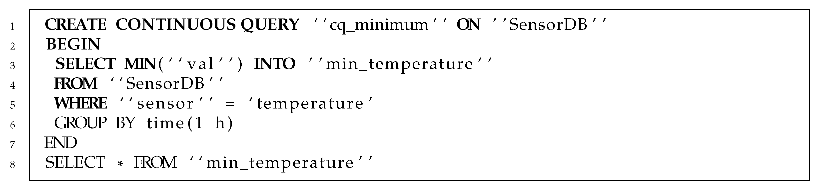
2.2.2. Query Language

InfluxDB provides the InfluxQL query language with SQL-like syntax. Figure 3 depicts an example of a query that finds the minimum value of the temperature sensor installed on the first machine.

As for mining tools, InfluxQL provides time series prediction through the Holt–Winters method [39]. Figure 4 shows an example of the prediction of the values of a temperature sensor.

InfluxDB supports continuous queries, which run automatically at a specified frequency. Figure 5 depicts an example of a continuous query that runs hourly and computes the minimum value of temperature sensor readings during an hour.

2.3. OpenTSDB, NoSQL-Based Time Series DBMS

OpenTSDB is a free TSDBMS implemented in the Java programming language. It serves as an add-on over NoSQL column family store systems, such as HBase or Cassandra [26]. OpenTSDB supports command line and HTTP interfaces, as well as client libraries and plugins [37].

2.3.1. Organization of Data Storage

OpenTSDB treats an element of a time series as a collection of a real value, a unique time series identifier (a metric in the original terminology), a timestamp, and a non-empty set of tags. A tag is a character string to store metadata.

OpenTSDB inherits the way the data are organized from the underlying NoSQL system, which uses a collection of system tables as a data storage, namely tsdb to manage data from time series, and tsdb-uid tsdb-tree, and tsdb-meta to manage service data. A tuple of the tsdb table contains the following attributes: a time series element, a timestamp, and a foreign key that references the table tsdb-uid and associates this tuple with a specific time series. The tsdb-uid table stores metric names and time-series tag values. In OpenTSDB, the tsdb-tree table allows for the definition and maintenance of a semantic hierarchy of stored time series similar to the file structure in an operating system. The tsdb-meta table allows for storing additional user-defined time-series information (for example, text annotations).

Figure 6 gives an example of the creation of a database for the subject domain from Figure 1, where OpenTSDB serves as an add-on over the HBase system. Initially, HBase runs a standard script to create system tables for data storage. Next, a database is created containing five metrics: acoustic, temperature, and accelerometer.x, accelerometer.y, and accelerometer.z, which represent the data from the respective sensors. Each of these metrics has a machine tag to indicate the device the sensor is installed on. The creation of the specified metrics is performed simultaneously with the insertion of data points to the database through the put command since OpenTSDB does not support explicit schema definition. The put command is followed by the metric name, timestamp, data point value, and tags.

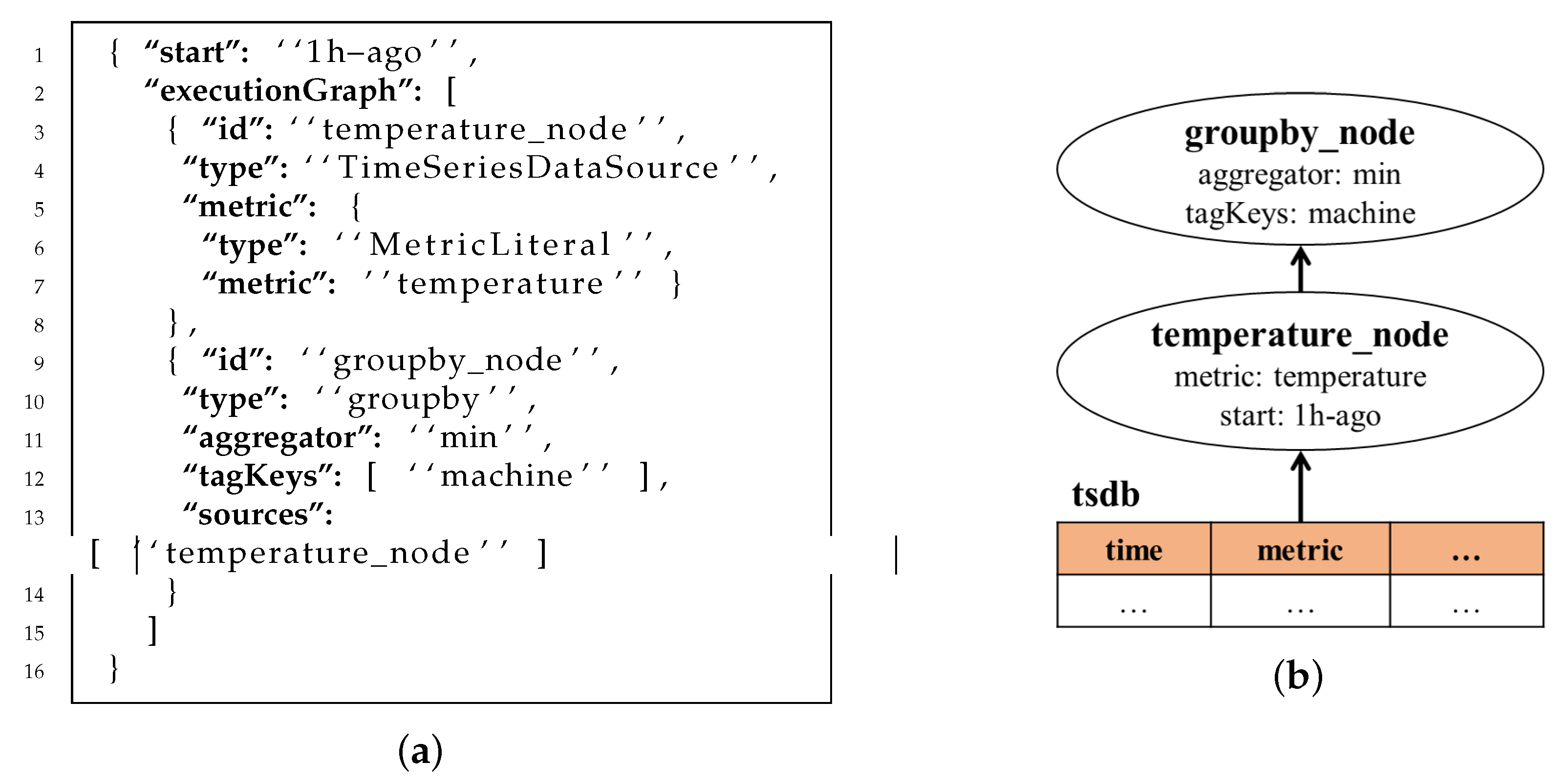
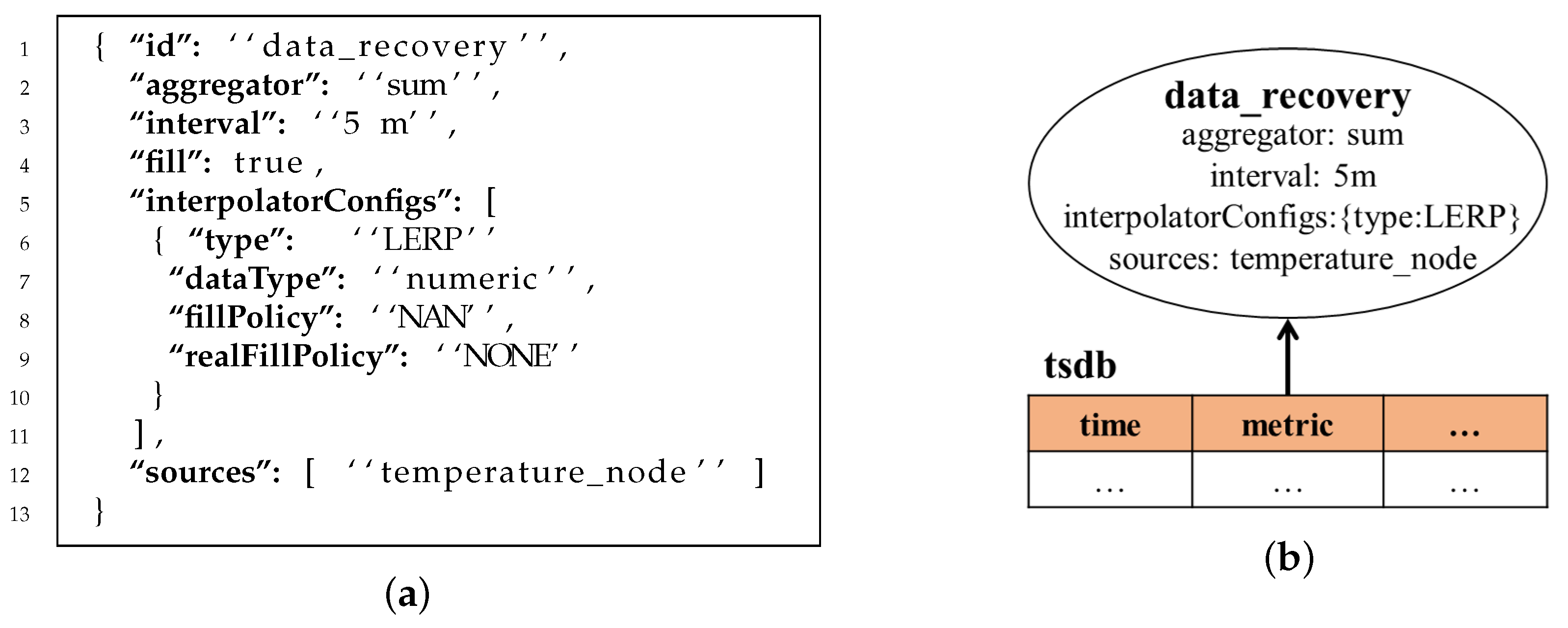
2.3.2. Query Language

In OpenTSDB, database queries are written in the JSON language. A query describes a directed acyclic graph (execution graph) whose nodes define data sources and transformation operations. The queries support arithmetic and logical expressions, filters, grouping, and others, as well as statistical and analytical functions, such as downsampling (decreasing the sampling rate of a series), interpolation (imputation of missing values of a series), and so forth.

Figure 7 shows an example of a query that performs grouping and computes the minimum value of temperature sensor data received in the last hour. The query graph consists of two nodes, namely temperature_node, which reads data from the temperature metric, and the groupby_node, which groups data by machine tag and finds the minimal value.

Figure 8 presents an example of a query that computes the total sum of data from the temperature_node metric grouped in 5 minute time intervals. In the resulting empty groups, the system automatically fills the gaps with the sum calculated by linear interpolation (LERP) [40]. If there is not enough real data for LERP, the system outputs an undefined value NaN.

Except for LERP, OpenTSDB does not provide built-in time series mining tools. However, OpenTSDB allows third-party extensions that provide such functionality (for example, the R2Time [41] library, implemented in the R programming language).

2.4. TimescaleDB, Relational-Based Time Series DBMS

TimescaleDB is a free TSDB implemented in the C programming language and distributed as an extension of PostgreSQL. TimescaleDB cooperates with a PostgreSQL instance and normally supports the same operations as PostgreSQL.

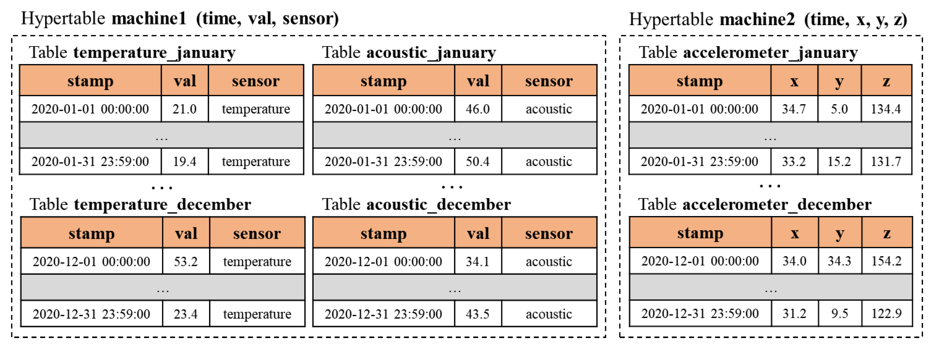
2.4.1. Organization of Data Storage

In TimescaleDB, time-series data are stored and processed in hypertables. A hypertable specifies a named set of time series and a way to split the data of the specified series into physically stored relational tables. The partitioning information is used further for parallel processing of the specified tables in PostgreSQL.

Figure 9 contains s the hypertables of data for the subject domain given in Figure 1. Here, each hypertable stores the time series of sensor data from the corresponding machine. The machine1 hypertable has the following attributes to store data from sensors installed on the first machine: a timestamp, a sensor value, and a sensor type (an acoustic emission sensor or a temperature sensor). The machine2 hypertable defines a way to store the vibration accelerometer data along the X, Y, and Z axes from the sensor installed on the second machine. Both hypertables define a time series split into disjoint subsequences corresponding to periods of one month. Additionally, the machine1 hypertable stores the data from different sensors in separate tables.

Figure 10 gives an example of the creation of a database in TimescaleDB with the hypertables shown in Figure 9. Initially, a new database and its tables are produced. Next, we employ TimescaleDB as a PostgreSQL extension and convert the tables into hypertables using the system function that specifies the partitioning method. Finally, sensor data are inserted in the hypertables through the regular SQL command INSERT.

2.4.2. Query Language

In TimescaleDB, data from hypertables are retrieved through the ordinary SQL SELECT command with a wide range of standard features, such as subqueries, sorting, grouping, and others. Additionally, in TimescaleDB, SQL is extended by facilities to perform statistical analysis of time series, namely calculating the median, the moving average, and percentiles, building histograms, grouping in time intervals of a given length, and so on.

Also, the TimescaleDB supports continuous aggregates, which are views to automatically compute and materialize the results of a specified query in the background. Continuous aggregates are similar to materialized views in PostgreSQL but, unlike the latter, they are updated automatically as data are inserted or modified. Figure 11 provides an example of a continuous aggregate that calculates the average value of temperature sensor data and groups these values in one-hour periods.

The TimescaleDB does not provide an application programmer with built-in time series mining functions. However, it inherits from PostgreSQL the ability to integrate with third-party libraries that implement data mining functions inside DBMS (for example, Apache MADlib [12]).

3. Mining Sensor Data Inside RDBMS

3.1. Matrix Profile Concept

The recently proposed Matrix Profile (MP) [16] is a data structure that annotates a time series through the index of and the distance to the nearest neighbor of each subsequence of the series. MP naturally allows one to detect both motifs and anomalies in a time series and can serve as a basis for discovering more sophisticated time-series mining primitives, such as semantic segments [42], chains (evolving patterns) [43], snippets (typical patterns) [44], and others.

Currently, MP and accompanying algorithms are extensively employed to mine sensor data in various Industry 4.0 applications. In [45], the authors describe how MP can be used to detect meter-swapping and prevent electricity theft. In [46], the authors present an MP-based approach to automatically labeling the system events in the synchrophasor data. In [47], MP is applied to discover discords in an energy time series for large commercial building load modeling. In [48], MP is applied to discover motifs and track the operational status of a machine through its vibration sensor data. In [49], the authors employ MP in Industrial IoT production maintenance.

Below, we follow [16,46], give basic definitions regarding MP, and thereafter describe an approach to embedding MP functionality into PostgreSQL.

Sensor data that undergo collection and mining are a form of time series.

Definition 1.

A time series is a chronologically ordered sequence of real-valued numbers: $T={\left\{t_i\right\}}_{i=1}^n$, where $t_i\in \mathbb{R}$.

Time series data mining is primarily addressed in discovering patterns of fixed relatively small length segments of a time series, or subsequences.

Definition 2.

A subsequence $T_{i,m}$ of a time series T is its subset of m successive elements that starts at the i-th position: $T_{i,m}={\left\{t_k\right\}}_{k=i}^{i+m-1}$, where $1\le i\le n-m+1$, and $1\le m\ll n$.

For further definitions, we specify all the subsequences of a given time series by sliding an m-length window throughout the time series (without physically extracting them).

Definition 3.

An all-subsequence set $S_T^A$ of a time series T is an ordered set of all possible m-length subsequences contained in T. Specifically, these subsequences are sorted in ascending order with respect to their starting elements: $S_T^A={\left\{T_{i,m}\right\}}_{i=1}^{n-m+1}$.

Next, for a given subsequence, we compute its distance to each element in an all-subsequence set.

Definition 4.

A distance profile $D_i^T$ is a vector of the distances between a given query subsequence $T_{i,m}$ and each subsequence $T_{j,m}$ in an all-subsequence set: $D_i^T={\left\{\mathit{dist}(T_{i,m},T_{j,m})\right\}}_{j=1}^{n-m+1}$, where $\mathit{dist}(·,·)$ denotes the Euclidean distance between z scores of two subsequences.

By the distance profile, we aim to find the nearest neighbor of each subsequence of a time series, except for trivial neighbors.

Definition 5.

A subsequence $T_{j,m}$ is the nearest neighbor of a subsequence $T_{i,m}$ if $\mathit{dist}(T_{i,m},T_{j,m})=min\left(D_i^T\right)$. A subsequence $T_{j,m}$ is a trivial neighbor of $T_{i,m}$ if $|i-j|\le \frac{m}{2}$.

Now, the matrix profile may be formally defined as follows.

Definition 6.

A matrix profile $P^T$ of a time series T is a vector of distances between each subsequence $T_{i,m}$ and its nearest nontrivial neighbor: $P^T={\left\{n{n}_{nt}\left(D_i^T\right)\right\}}_{i=1}^{n-m+1}$, where $n{n}_{nt}\left(D_i^T\right)$ denotes the minimal distance between $T_{i,m}$ and its nontrivial neighbors.

A matrix profile is accompanied by a supplemental structure to locate the nearest nontrivial neighbors.

Definition 7.

A matrix profile index $I^T$ of a time series T is a vector that stores the index of the nearest nontrivial neighbor of each subsequence: $I^T={\left\{I_i^T\right\}}_{i=1}^{n-m+1}$, where $I_i^T=j$ if $n{n}_{nt}\left(D_i^T\right)=\mathit{dist}(T_{i,m},T_{j,m})$.

The matrix profile can be considered as metadata to annotate corresponding time series. For example, the maximal value of the profile corresponds to an anomalous subsequence (a discord [50]), whereas the minimal values correspond to the best motif subsequence pair in the series.

The matrix profile and the matrix profile index can be generalized to the case of two time series when the query subsequence and the all-subsequence set are taken from different time series. In this case, we call $P^{T1,T2}$ and $I^{T1,T2}$ the join matrix profile and the join matrix profile index, respectively. Commonly, $P^{T1,T2}\ne P^{T2,T1}$ and $I^{T1,T2}\ne I^{T2,T1}$.

The matrix profile is a domain-agnostic technique where an application programmer specifies the only parameter (a subsequence length). Among other advantages, the matrix profile allows for its parallel computing [51] and gradual updating [45].

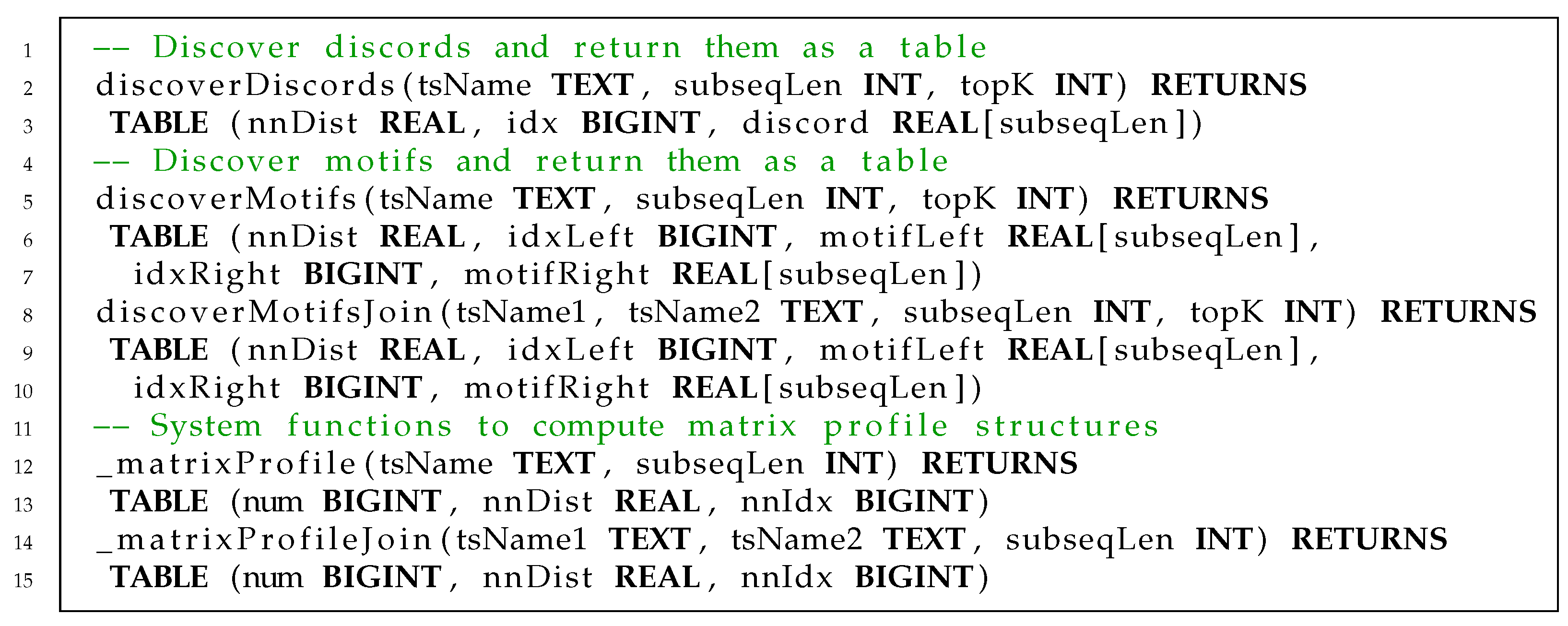
3.2. Embedding Matrix Profile Management into RDBMS

Embedding MP functionality into RDBMS has two basic merits. By encapsulating time series data mining inside DBMS, we avoid overheads due to export–import large data. Moreover, being computed and stored in the database once, a matrix profile and related time series data mining primitives can then be used repeatedly.

To embed MP functionality into RDBMS, we represent a sensor database as depicted in Figure 12. Time series data are represented by the Time Series Directory (TSD) table, a set of univariate time series tables, and a set of multivariate time series tables. The TSD table stores information on each time series, namely its dimension, length, and the name of the table. Each univariate time series is implemented as a table with columns representing a serial number, a timestamp, and a sensor value itself. A multivariate time series is implemented as a table with a similar structure where each dimension is represented as a real-valued column.

Matrix Profile data consist of the Matrix Profile Directory (MPD) table, a set of Matrix Profile (MP) tables, a set of Join Matrix Profile (JMP) tables, and a set of Distance Profiles (DP) tables. The MPD table stores metadata on the matrix profiles managed within the system and references corresponding time series in the TSD table (one or two foreign keys for an ordinary or join matrix profile, respectively). Each MP table, in the same manner as a JMP table, stores one matrix profile of the stored time series for a given subsequence length, using to this end one real-valued column for the distance to the nearest neighbor subsequence and one integer-valued column for the index thereof (that is, the MP table also stores a matrix profile index). Each DP table stores all the distance profiles of a time series for a given subsequence length, using for this purpose two integer-valued columns for the indices of subsequences and one real-valued column for the distance between them. The naming of Matrix Profile data objects reflects their indirect connection to Time series data objects and the subsequence length. For example, let us store acoustic sensor data in the ts_acoustic table and let us mine these data along 128-length subsequences. Then the sensor database contains the mp_acoustic_128 table and the dp_acoustic_128 table to store the Matrix Profile and the Distance Profiles of the time series, respectively.

The Time series data mining (TSDM) API provides an application programmer with tools to discover discords and motifs and compute matrix profiles. Similar to TimescaleDB, our API (which was called MPPostgres) is implemented as a PostgreSQL extension consisting of PL/pgSQL functions that return tables (see Figure 13). PL/pgSQL (Procedural Language/PostgreSQL) is a fully featured programming language that supported by PostgreSQL and allows much more procedural control than traditional SQL.

In MPPostgres, a discord table representation includes the following items: the index of the discord in the time series, the distance to its nearest neighbor, and the discord itself as an array. A motif is represented as a tuple with the following attributes: the left and right parts of the motif, their indices, and the distance between them. A PL/pgSQL function result can be stored in the database as a table or exploited as a view (virtual table). The API can be complemented with functions to search for other mining primitives (chains, snippets, etc.). Discords and motifs are computed through SQL queries that select the rows of the MP table with the maximal and minimal values of the distance to the nearest neighbor (the nnDist column), respectively. The PL/pgSQL functions to compute matrix profiles are implemented as wrappers over the in-memory algorithm [51]. Note that such PL/pgSQL function is implemented in such a manner that it is called only if the respective MP table has not been created yet.

MPPostgres can seamlessly work in tandem with TimescaleDB on top of PostgreSQL, as the example in Figure 14 shows (cf. Figure 10; note that, for the sake of simplicity, we have left only one sensor). After the typical steps (create a database in PostgreSQL, employ TimescaleDB, transform tables into hypertables, and insert sensor data in hypertables), we employ MPPostgres to discover discords and motifs based on the matrix profile and display the findings.

4. Experimental Case Studies

We embedded MP functionality into PostgreSQL v. 13.2 and evaluated the proposed approach in experiments conducted on a workstation (CPU: Intel Xeon Gold 6254 @4 GHz, RAM: 64 Gb, HDD: 1 Tb). In the experiments, we considered three cases of real Industry 4.0 applications related to mining big sensor data and implemented them based on the proposed approach. In these cases, we assumed that sensor data were stored and mined inside PostgreSQL and assessed the performance (running time) of our approach. We also compared our results with those of solutions based on InfluxDB and OpenTSDB, assuming that the sensor data were firstly exported outside these TSDBMSs, then converted to an appropriate format and mined with third-party tools [52], and finally, the results were imported back into those TSDBMSs. We keep in mind the fact that out-of-TSDBMS time series data mining is potentially faster than the in-TSDBMS one, but the absence of export-import overhead costs in our approach allows us to hope for an eventual advantage.

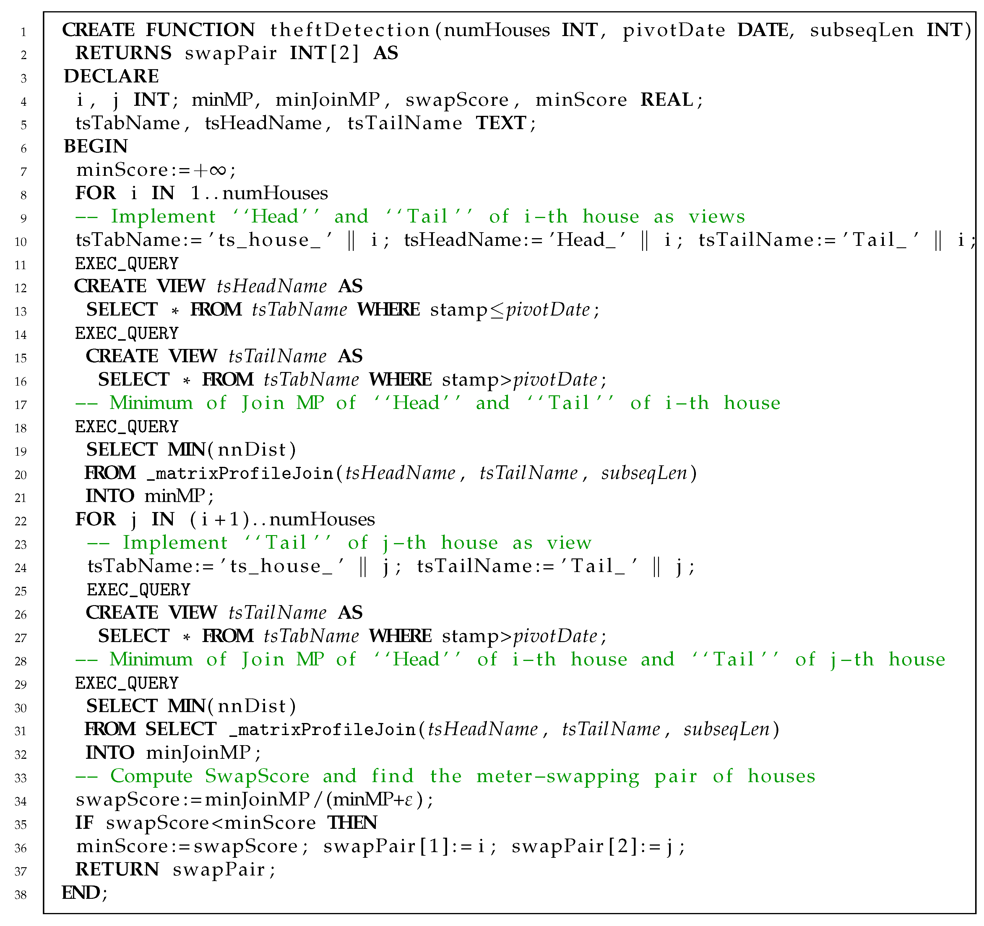
4.1. Electricity Theft Detection

In [45], the authors exploit the matrix profile concept to detect electricity theft. They simulate a meter-swapping event in a dataset of household electric power demand collected from twenty households [53] by swapping the traces of two time series (chosen randomly) starting at a specific date. Next, to discover the swapped pair, they divide each time series into two sections: the “Head”, before the selected date, and the “Tail”, after that date. Finally, among all possible pairs of houses, the resulting pair $\{{\mathrm{House}}_i,{\mathrm{House}}_j\}$ should have the minimal swap-score, which is computed as

$$\mathrm{SwapScore}({\mathrm{House}}_i,{\mathrm{House}}_j)=\frac{min\left(P^{\mathrm{Head}\left({\mathrm{House}}_i\right),\mathrm{Tail}\left({\mathrm{House}}_j\right)}\right)}{min\left(P^{\mathrm{Head}\left({\mathrm{House}}_i\right),\mathrm{Tail}\left({\mathrm{House}}_i\right)}\right)+\epsilon },$$

where $\epsilon$ denotes the machine epsilon (an upper bound on the relative error due to rounding in floating-point arithmetic).

Figure 15 shows how we implemented that case in MPPostgres (here and below, we use pseudo-code with a PL/pgSQL-like syntax, where the $\mathtt{EXEC}\_\mathtt{QUERY}$ statement runs a query with a specified character string, and an italicized variable name denotes the value of the respective variable, rather than the query text that is actually written). Note that all “Head”s and “Tail”s are represented by views (virtual tables), so we do not have overheads caused by physically extracting them for further processing.

Figure 16 shows experimental results associated with the electricity theft detection case. It can be seen that all the competitors perform matrix profile computations of the same duration. MPPostgres requires a short-time preprocessing for extracting data from tables through SQL queries. Also, all the solutions perform auxiliary computations (finding the minimum, computing $\mathit{SwapScore}$, etc.), where MPPostgres is slightly ahead of rivals. Finally, data export (extraction of data and its transference to a third-party application) introduces significant overheads due to out-of-TSDBMS solutions and is absent in our approach.

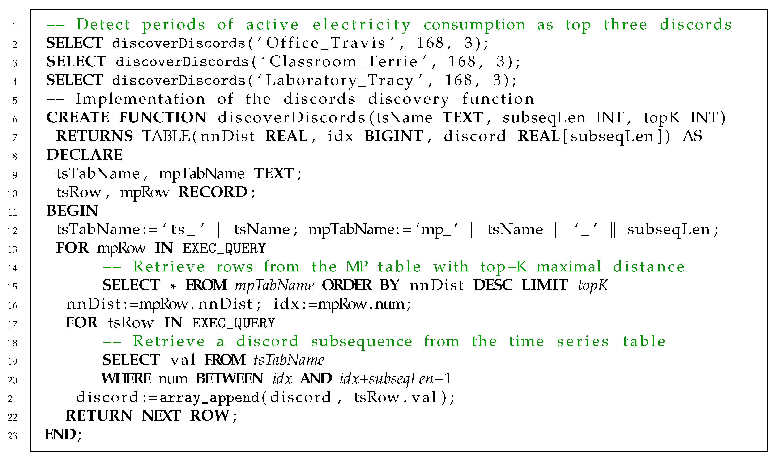
4.2. Detection of Active Electricity Consumption

The authors of [47] apply the matrix profile concept for modeling electricity consumption in three buildings of an academic campus located in Zurich, Switzerland. The authors exploit the Building Data Genome (BDG) dataset [54], where the reference buildings represent an office, a classroom, and a laboratory, identified through their nicknames: Travis, Tracy, and Teri, respectively. Among other things, the authors determine for each building the periods of active electricity consumption by discovering the top three discords as maximal points in the matrix profile of the consumer-side building electric power time series, where the subsequence length parameter corresponds to one week (seven days of hourly readings and a total of 168 points).

The implementation of the case in MPPostgres is shown in Figure 17. To find the discords, we simply call the $\mathtt{discoverDiscords}$ function of the TSDM API three times, specifying the respective parameters. The remaining code shows how the above-mentioned function is implemented. The rows of the resulting table are formed through the following loop. Using an SQL query, we select the rows with top-K maximal distance to the nearest neighbor from the MP table and take the values of the index and the distance fields for a row of the resulting table. At last, using the index found, we select all the points of the respective discord subsequence by an SQL query.

Figure 18 depicts the experimental results associated with the case of active electricity consumption in buildings (for illustrative purposes, we replicated the BDG dataset, so that it corresponds to data for 32 years). We can observe a situation similar to the previous case. All the competitors compute the matrix profile equally fast. According to their nature, out-of-TSDBMS solutions introduce significant overhead costs on data export, in contrast to our approach. MPPostgres also outperforms the rivals at the discord discovery step since it exploits the built-in database indexing by table primary key when finding top-K values and retrieving rows from tables. It is worth noting that in the typical scenario, when the matrix profile has already been computed and saved in the MP table, our approach would outperform our rivals even more significantly.

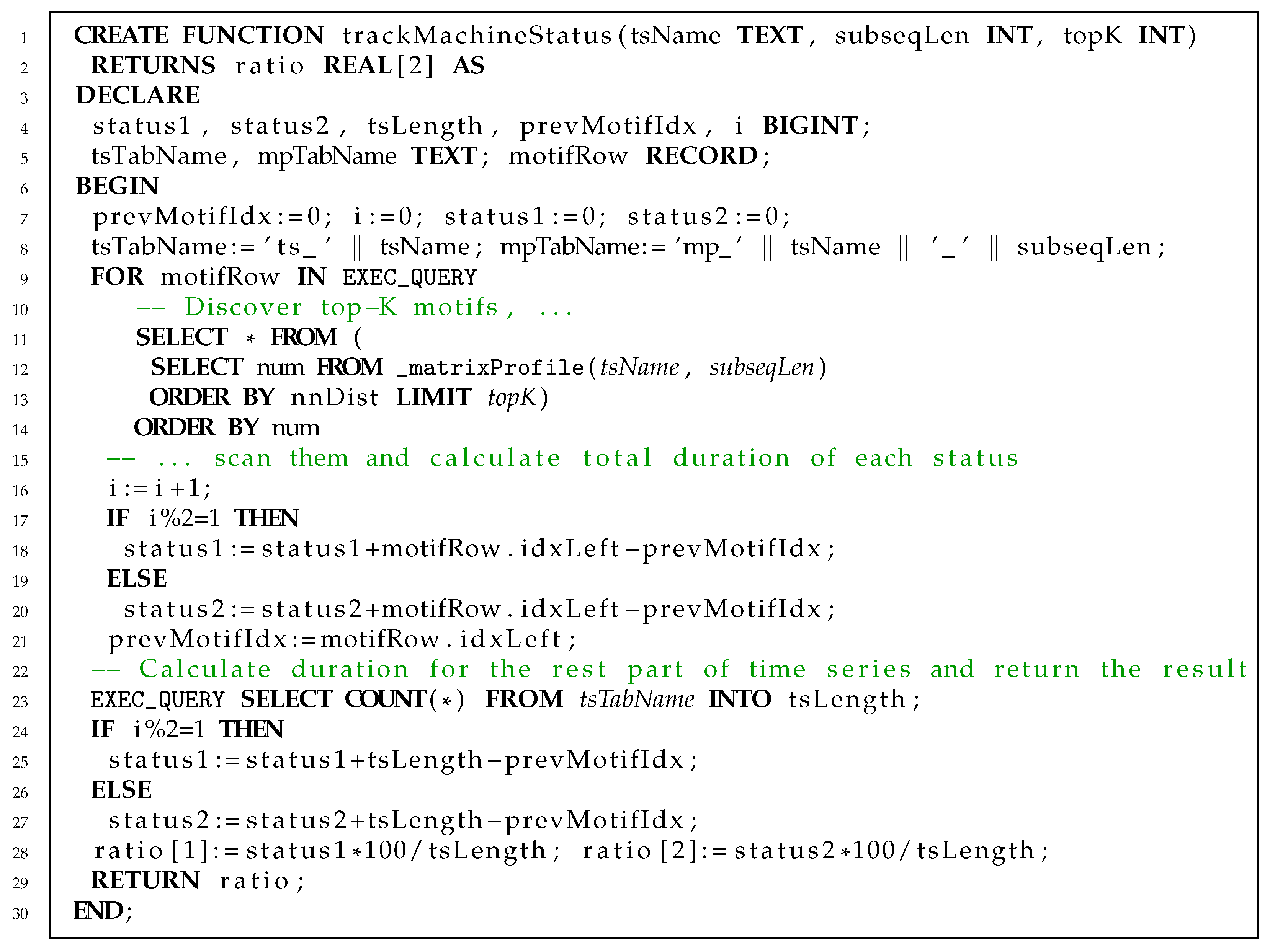
4.3. Tracking the Operational Status of an Industrial Machine

The authors of [48] track the operational status of an industrial two-mode (high and low speed) exhaust fan through the matrix profile computed for a time series collected by a vibration sensor installed on the fan. While collecting the data, the authors deliberately control the fan blowing duration and speed. Switching the fan modes affects the vibrations, while the motifs in the time series indicate the moments when the machine status changes. The authors discover motifs through the matrix profile and compute the total duration of time intervals when the fan is in “high-speed” and “low-speed” mode, as well as the ratio of such intervals. The experimental results show that the ratio computed through the matrix profile is almost identical to ground truth data.

The authors of [48] do not provide the vibration dataset. We conducted in our study experiments similar to the one described in [48] and collected vibration data from a small-sized crushing machine which is located at the South Ural State University (Chelyabinsk, Russia) and is used for training engineers. The collected time series consists of more than 240 thousand points corresponding to a 3 minute time interval of machine work. During the process, we started up the crushing machine eight times, so that the machine status changed sixteen times, from “crushing stops” to “crushing starts” and back. As in the original case, the ratio of time intervals when the machine works in different modes, computed in our experiments through motif discovery, almost coincides with ground truth data.

The implementation of the described case in MPPostgres is shown in Figure 19. After computing the matrix profile of an input time series, we use an SQL query to retrieve top-K motifs as rows of the MP table with top-K minimal distance to the nearest neighbor of the respective subsequence. Then, we scan the time series from left to right through the indices of motifs found while computing the length of the interval between the previous and current motif and alternately adding the result to a total duration that indicates when the machine works in the first or the second mode. Finally, after similar one-time computations over the remaining part of the input time series, we obtain the resulting ratio.

In Figure 20, we see the experimental results obtained in the crushing machine operational status tracking case. Similar to previous cases, MPPostgres outperforms the out-of-TSDBMS rivals since the latter are forced to export the data before processing it. Also, in the typical scenario when the matrix profile has already been computed and saved in the MP table, MPPostgres would show even higher performance.

5. Conclusions

In this article, we addressed the problem of choosing an appropriate tool for managing and mining big sensor data. Currently, such data arise in a wide spectrum of Industry 4.0 and Internet of Things applications, such as predictive maintenance, smart cities and factories, digital twins, and others. Such sensors have high frequency and produce time series containing up to tens of millions of elements in a relatively short time interval. The data collected from the sensors are subject to mining in order to make strategic decisions. To efficiently do this, we need specific Time Series DBMSs (TSDBMSs), which differ from relational DBMSs (RDBMSs) and NoSQL systems.

We suggest distinguishing native and add-on TSDBMSs. A native TSDBMS is a stand-alone development with an original query language, a database engine, and a data storage system. An add-on TSDBMS is implemented on top of a third-party system that provides the TSDBMS with a database engine and a data storage system. We briefly described the most popular representatives of the above-mentioned categories: InfluxDB (native TSDBMS), OpenTSDB (add-on over a NoSQL system), and TimescaleDB (add-on over a relational DBMS). Our overview showed that the above-mentioned systems provide an application programmer with a modest built-in toolset to mine time series data. This leads to unwanted overhead costs since we should use third-party mining systems that need to connect to a sensor database server first, then export the data outside the TSDBMS, convert them to an appropriate format before mining, and finally, import the results back into the TSDBMS.

We presented an approach to managing and mining sensor data inside RDBMS based on the Matrix Profile concept [16]. The Matrix Profile annotates a time series through the index of and the distance to the nearest neighbor of each subsequence of the time series. The Matrix Profile serves as a basis to discover motifs and discords in time series. Sensor data are stored as a set of univariate and multivariate time series tables, and their metadata are provided by the Time Series Directory table. Moreover, the sensor database contains tables to store the Matrix Profile data and the Matrix Profile Directory table to store metadata. We implemented this approach as a PostgreSQL extension which provides an application programmer with a set of user-defined functions (UDFs) to compute a matrix profile and time series data mining primitives and represent them as relational tables.

To evaluate the suggested approach, we performed an experimental study of three cases of real Industry 4.0 applications related to mining big sensor data, namely electricity meter-swapping detection, determining of active electricity consumption in buildings, and tracking operational status of machines. We assessed the performance of our approach against solutions based on InfluxDB and OpenTSDB. Our approach surpassed these out-of-TSDBMS competitors since it assumes that sensor data are mined inside a TSDBMS at no significant overhead costs due to data export and conversion, etc.

In further studies, we plan to enhance our TSDBMS extension of PostgreSQL with other sophisticated time series primitives, such as semantic segments, evolving and typical patterns, and others.

References

1. Xu, L.D.; Duan, L. Big Data for cyber physical systems in Industry 4.0: A survey. Enterp. Inf. Syst. 2019, 13, 148–169. [Google Scholar] [CrossRef]
2. Kumar, S.; Tiwari, P.; Zymbler, M.L. Internet of Things is a revolutionary approach for future technology enhancement: A review. J. Big Data 2019, 6, 111. [Google Scholar] [CrossRef] [Green Version]
3. Ivanov, S.; Nikolskaya, K.; Radchenko, G.; Sokolinsky, L.; Zymbler, M. Digital twin of city: Concept overview. In Proceedings of the 2020 Global Smart Industry Conference, GloSIC 2020, Chelyabinsk, Russia, 17–19 November 2020; pp. 178–186. [Google Scholar] [CrossRef]
4. Zymbler, M.; Kraeva, Y.; Latypova, E.; Kumar, S.; Shnayder, D.; Basalaev, A. Cleaning sensor data in smart heating control system. In Proceedings of the 2020 Global Smart Industry Conference, GloSIC 2020, Chelyabinsk, Russia, 17–19 November 2020; pp. 375–381. [Google Scholar] [CrossRef]
5. Ordonez, C. Can we analyze big data inside a DBMS? In Proceedings of the 16th International Workshop on Data Warehousing and OLAP, DOLAP 2013, San Francisco, CA, USA, 28 October 2013; Song, I., Bellatreche, L., Cuzzocrea, A., Eds.; 2013; pp. 85–92. [Google Scholar] [CrossRef]
6. Baralis, E.; Cerquitelli, T.; Chiusano, S. Index Support for Frequent Itemset Mining in a Relational DBMS. In Proceedings of the 21st International Conference on Data Engineering, ICDE 2005, Tokyo, Japan, 5–8 April 2005; Aberer, K., Franklin, M.J., Nishio, S., Eds.; 2005; pp. 754–765. [Google Scholar] [CrossRef]
7. Sidló, C.I.; Lukács, A. Shaping SQL-Based Frequent Pattern Mining Algorithms. In Proceedings of the Knowledge Discovery in Inductive Databases, 4th International Workshop, (KDID 2005), Porto, Portugal, 3 October 2005; Revised Selected and Invited Papers; Lecture Notes in Computer Science. Bonchi, F., Boulicaut, J., Eds.; Springer: Berlin, Germany, 2005; Volume 3933, pp. 188–201. [Google Scholar] [CrossRef]
8. Pelekis, N.; Tampakis, P.; Vodas, M.; Panagiotakis, C.; Theodoridis, Y. In-DBMS Sampling-based Sub-trajectory Clustering. In Proceedings of the 20th International Conference on Extending Database Technology, EDBT 2017, Venice, Italy, 21–24 March 2017; Markl, V., Orlando, S., Mitschang, B., Andritsos, P., Sattler, K., Breß, S., Eds.; 2017; pp. 632–643. [Google Scholar] [CrossRef]
9. Zymbler, M.L.; Kraeva, Y.; Grents, A.; Perkova, A.; Kumar, S. An Approach to Fuzzy Clustering of Big Data Inside a Parallel Relational DBMS. In Proceedings of the Data Analytics and Management in Data Intensive Domains—21st International Conference, DAMDID/RCDL 2019, Kazan, Russia, 15–18 October 2019; Revised Selected Papers; Communications in Computer and Information Science. Elizarov, A.M., Novikov, B., Stupnikov, S.A., Eds.; Springer: Berlin, Germany, 2019; Volume 1223, pp. 211–223. [Google Scholar] [CrossRef]
10. Pan, C.S.; Zymbler, M.L. Very Large Graph Partitioning by Means of Parallel DBMS. In Proceedings of the Advances in Databases and Information Systems—17th East European Conference, ADBIS 2013, Genoa, Italy, 1–4 September 2013; Catania, B., Guerrini, G., Pokorný, J., Eds.; Lecture Notes in Computer Science. Springer: Berlin, Germany, 2013; Volume 8133, pp. 388–399. [Google Scholar] [CrossRef]
11. McCaffrey, J.D. A Hybrid System for Analyzing Very Large Graphs. In Proceedings of the 9th International Conference on Information Technology: New Generations (ITNG 2012), Las Vegas, NV, USA, 16–18 April 2012; Latifi, S., Ed.; pp. 253–257. [Google Scholar] [CrossRef]
12. Hellerstein, J.M.; Ré, C.; Schoppmann, F.; Wang, D.Z.; Fratkin, E.; Gorajek, A.; Ng, K.S.; Welton, C.; Feng, X.; Li, K.; et al. The MADlib Analytics Library or MAD Skills, the SQL. Proc. VLDB Endow. 2012, 5, 1700–1711. [Google Scholar] [CrossRef]
13. Feng, X.; Kumar, A.; Recht, B.; Ré, C. Towards a unified architecture for in-RDBMS analytics. In Proceedings of the ACM SIGMOD International Conference on Management of Data, SIGMOD 2012, Scottsdale, AZ, USA, 20–24 May 2012; pp. 325–336. [Google Scholar] [CrossRef] [Green Version]
14. Mahajan, D.; Kim, J.K.; Sacks, J.; Ardalan, A.; Kumar, A.; Esmaeilzadeh, H. In-RDBMS Hardware Acceleration of Advanced Analytics. Proc. VLDB Endow. 2018, 11, 1317–1331. [Google Scholar] [CrossRef] [Green Version]
15. Rechkalov, T.; Zymbler, M.L. Integrating DBMS and Parallel Data Mining Algorithms for Modern Many-Core Processors. In Proceedings of the Data Analytics and Management in Data Intensive Domains—XIX International Conference (DAMDID/RCDL 2017), Moscow, Russia, 10–13 October 2017; Revised Selected Papers; Communications in Computer and Information Science. Kalinichenko, L.A., Manolopoulos, Y., Malkov, O., Skvortsov, N.A., Stupnikov, S.A., Sukhomlin, V., Eds.; Springer: Berlin, Germany, 2017; Volume 822, pp. 230–245. [Google Scholar] [CrossRef]
16. Yeh, C.M.; Zhu, Y.; Ulanova, L.; Begum, N.; Ding, Y.; Dau, H.A.; Zimmerman, Z.; Silva, D.F.; Mueen, A.; Keogh, E.J. Time series joins, motifs, discords and shapelets: A unifying view that exploits the matrix profile. Data Min. Knowl. Discov. 2018, 32, 83–123. [Google Scholar] [CrossRef]
17. Bader, A.; Kopp, O.; Falkenthal, M. Survey and Comparison of Open Source Time Series Databases; Datenbanksysteme fur Business, Technologie und Web (BTW 2017), 17. Fachtagung des GI-Fachbereichs “Datenbanken und Informationssysteme” (DBIS), 6.–10. Marz 2017, Stuttgart, Germany, Workshopband; Mitschang, B., Ritter, N., Schwarz, H., Klettke, M., Thor, A., Kopp, O., Wieland, M., Eds.; Gesellschaft für Informatik e.V.: Bonn, Germany, 2017; pp. 249–268. [Google Scholar]
18. Grzesik, P.; Mrozek, D. Comparative analysis of time series databases in the context of Edge computing for low power sensor networks. In Proceedings of the 20th International Conference on Computational Science (ICCS 2020), Amsterdam, The Netherlands, 3–5 June 2020; pp. 371–383. [Google Scholar] [CrossRef]
19. Yang, F.; Tschetter, E.; Léauté, X.; Ray, N.; Merlino, G.; Ganguli, D. Druid: A real-time analytical data store. In Proceedings of the International Conference on Management of Data (SIGMOD 2014), Snowbird, UT, USA, 22–27 June 2014; Dyreson, C.E., Li, F., Ozsu, M.T., Eds.; ACM: New York, NY, USA, 2014; pp. 157–168. [Google Scholar] [CrossRef]
20. Rhea, S.; Wang, E.; Wong, E.; Atkins, E.; Storer, N. LittleTable: A Time-Series Database and Its Uses. In Proceedings of the 2017 ACM International Conference on Management of Data (SIGMOD Conference 2017), Chicago, IL, USA, 14–19 May 2017; Salihoglu, S., Zhou, W., Chirkova, R., Yang, J., Suciu, D., Eds.; 2017; pp. 125–138. [Google Scholar] [CrossRef]
21. Li, C.; Li, B.; Bhuiyan, M.Z.A.; Wang, L.; Si, J.; Wei, G.; Li, J. FluteDB: An efficient and scalable in-memory time series database for sensor-cloud. J. Parallel Distributed Comput. 2018, 122, 95–108. [Google Scholar] [CrossRef]
22. MacDonald, A. PhilDB: The time series database with built-in change logging. PeerJ Comput. Sci. 2016, 2, e52. [Google Scholar] [CrossRef] [Green Version]
23. Yang, Y.; Cao, Q.; Jiang, H. EdgeDB: An Efficient Time-Series Database for Edge Computing. IEEE Access 2019, 7, 142295–142307. [Google Scholar] [CrossRef]
24. Lan, L.; Shi, R.; Wang, B.; Zhang, L.; Shi, J. A Lightweight Time Series Main-Memory Database for IoT Real-Time Services. In Proceedings of the Internet of Vehicles, Technologies and Services Toward Smart Cities—6th International Conference (IOV 2019), Kaohsiung, Taiwan, 18–21 November 2019; Lecture Notes in Computer Science. Hsu, C., Khemiri-Kallel, S., Lan, K., Zheng, Z., Eds.; Springer: Berlin, Germany, 2019; Volume 11894, pp. 220–236. [Google Scholar] [CrossRef]
25. Pelkonen, T.; Franklin, S.; Cavallaro, P.; Huang, Q.; Meza, J.; Teller, J.; Veeraraghavan, K. Gorilla: A Fast, Scalable, In-Memory Time Series Database. Proc. VLDB Endow. 2015, 8, 1816–1827. [Google Scholar] [CrossRef]
26. Matallah, H.; Belalem, G.; Bouamrane, K. Evaluation of NoSQL Databases: MongoDB, Cassandra, HBase, Redis, Couchbase, OrientDB. Int. J. Softw. Sci. Comput. Intell. 2020, 12, 71–91. [Google Scholar] [CrossRef]
27. Andersen, M.P.; Culler, D.E. BTrDB: Optimizing Storage System Design for Timeseries Processing. In Proceedings of the 14th USENIX Conference on File and Storage Technologies (FAST 2016), Santa Clara, CA, USA, 22–25 February 2016; Brown, A.D., Popovici, F.I., Eds.; 2016; pp. 39–52. [Google Scholar]
28. Shvachko, K.; Kuang, H.; Radia, S.; Chansler, R. The Hadoop Distributed File System. In Proceedings of the IEEE 26th Symposium on Mass Storage Systems and Technologies (MSST 2012), Lake Tahoe, NV, USA, 3–7 May 2010; Khatib, M.G., He, X., Factor, M., Eds.; 2010; pp. 1–10. [Google Scholar] [CrossRef]
29. Sim, H.; Khan, A.; Vazhkudai, S.S.; Lim, S.; Butt, A.R.; Kim, Y. An Integrated Indexing and Search Service for Distributed File Systems. IEEE Trans. Parallel Distrib. Syst. 2020, 31, 2375–2391. [Google Scholar] [CrossRef]
30. Idreos, S.; Groffen, F.; Nes, N.; Manegold, S.; Mullender, K.S.; Kersten, M.L. MonetDB: Two Decades of Research in Column-oriented Database Architectures. IEEE Data Eng. Bull. 2012, 35, 40–45. [Google Scholar]
31. Deri, L.; Mainardi, S.; Fusco, F. tsdb: A Compressed Database for Time Series. In Proceedings of the Traffic Monitoring and Analysis—4th International Workshop (TMA 2012), Vienna, Austria, 12 March 2012; Lecture Notes in Computer Science. Pescapè, A., Salgarelli, L., Dimitropoulos, X.A., Eds.; Springer: Berlin, Germany, 2012; Volume 7189, pp. 143–156. [Google Scholar] [CrossRef] [Green Version]
32. Seltzer, M.I. Berkeley DB: A Retrospective. IEEE Data Eng. Bull. 2007, 30, 21–28. [Google Scholar]
33. Tsubouchi, Y.; Wakisaka, A.; Hamada, K.; Matsuki, M.; Abe, H.; Matsumoto, R. HeteroTSDB: An Extensible Time Series Database for Automatically Tiering on Heterogeneous Key-Value Stores. In Proceedings of the 43rd IEEE Annual Computer Software and Applications Conference (COMPSAC 2019), Milwaukee, WI, USA, 15–19 July 2019; Getov, V., Gaudiot, J., Yamai, N., Cimato, S., Chang, J.M., Teranishi, Y., Yang, J., Leong, H.V., Shahriar, H., Takemoto, M., et al., Eds.; 2019; Volume 1, pp. 264–269. [Google Scholar] [CrossRef]
34. Sivasubramanian, S. Amazon dynamoDB: A seamlessly scalable non-relational database service. In Proceedings of the ACM SIGMOD International Conference on Management of Data (SIGMOD 2012), Scottsdale, AZ, USA, 20–24 May 2012; pp. 729–730. [Google Scholar] [CrossRef]
35. Stonebraker, M.; Rowe, L.A.; Hirohama, M. The implementation of POSTGRES. In Making Databases Work: The Pragmatic Wisdom of Michael Stonebraker; Brodie, M.L., Ed.; ACM/Morgan & Claypool: San Rafael, CA, USA, 2019; pp. 519–559. [Google Scholar] [CrossRef] [Green Version]
36. Arous, I.; Khayati, M.; Cudré-Mauroux, P.; Zhang, Y.; Kersten, M.L.; Stalinlov, S. RecovDB: Accurate and Efficient Missing Blocks Recovery for Large Time Series. In Proceedings of the 35th IEEE International Conference on Data Engineering (ICDE 2019), Macao, China, 8–11 April 2019; pp. 1976–1979. [Google Scholar] [CrossRef]
37. Petre, I.; Boncea, R.; Radulescu, C. A time-series database analysis based on a multi-attribute maturity model. Stud. Inf. Control 2019, 2, 177–188. [Google Scholar] [CrossRef] [Green Version]
38. O’Neil, P.E.; Cheng, E.; Gawlick, D.; O’Neil, E.J. The Log-Structured Merge-Tree (LSM-Tree). Acta Inf. 1996, 33, 351–385. [Google Scholar] [CrossRef]
39. Holt, C. Forecasting seasonals and trends by exponentially weighted averages. Int. J. Forecast. 2004, 20, 5–10. [Google Scholar] [CrossRef]
40. Petersen, D.P.; Middleton, D. Linear interpolation, extrapolation, and prediction of random space-time fields with a limited domain of measurement. IEEE Trans. Inf. Theory 1965, 11, 18–30. [Google Scholar] [CrossRef]
41. Agrawal, B.; Chakravorty, A.; Rong, C.; Wlodarczyk, T.W. R2Time: A Framework to Analyse Open TSDB Time-Series Data in HBase. In Proceedings of the IEEE 6th International Conference on Cloud Computing Technology and Science (CloudCom 2014), Singapore, 15–18 December 2014; pp. 970–975. [Google Scholar] [CrossRef]
42. Gharghabi, S.; Ding, Y.; Yeh, C.M.; Kamgar, K.; Ulanova, L.; Keogh, E.J. Matrix Profile VIII: Domain Agnostic Online Semantic Segmentation at Superhuman Performance Levels. In Proceedings of the 2017 IEEE International Conference on Data Mining (ICDM 2017), New Orleans, LA, USA, 18–21 November 2017; pp. 117–126. [Google Scholar] [CrossRef]
43. Zhu, Y.; Imamura, M.; Nikovski, D.; Keogh, E.J. Matrix Profile VII: Time Series Chains: A New Primitive for Time Series Data Mining. In Proceedings of the 2017 IEEE International Conference on Data Mining, ICDM 2017, New Orleans, LA, USA, 18–21 November 2017; pp. 695–704. [Google Scholar] [CrossRef]
44. Imani, S.; Madrid, F.; Ding, W.; Crouter, S.E.; Keogh, E.J. Matrix Profile XIII: Time Series Snippets: A New Primitive for Time Series Data Mining. In Proceedings of the 2018 IEEE International Conference on Big Knowledge, ICBK 2018, Singapore, 17–18 November 2018; Wu, X., Ong, Y., Aggarwal, C.C., Chen, H., Eds.; 2018; pp. 382–389. [Google Scholar] [CrossRef]
45. Zhu, Y.; Gharghabi, S.; Silva, D.F.; Dau, H.A.; Yeh, C.M.; Senobari, N.S.; Almaslukh, A.; Kamgar, K.; Zimmerman, Z.; Funning, G.J.; et al. The Swiss army knife of time series data mining: Ten useful things you can do with the matrix profile and ten lines of code. Data Min. Knowl. Discov. 2020, 34, 949–979. [Google Scholar] [CrossRef]
46. Shi, J.; Yu, N.; Keogh, E.; Chen, H.; Yamashita, K. Discovering and Labeling Power System Events in Synchrophasor Data with Matrix Profile. In Proceedings of the 2019 IEEE Sustainable Power and Energy Conference (iSPEC), Beijing, China, 21–23 November 2019; p. 19303617. [Google Scholar] [CrossRef]
47. Nichiforov, C.; Stancu, I.; Stamatescu, I.; Stamatescu, G. Information Extraction Approach for Energy Time Series Modelling. In Proceedings of the 24th International Conference on System Theory, Control and Computing (ICSTCC 2020), Sinaia, Romania, 8–10 October 2020; Barbulescu, L., Ed.; 2020; pp. 886–891. [Google Scholar] [CrossRef]
48. Lee, Y.Q.; Beh, W.L.; Ooi, B.Y. Tracking Operation Status of Machines through Vibration Analysis using Motif Discovery. J. Phys. Conf. Ser. 2020, 1529, 052005. [Google Scholar] [CrossRef]
49. Pizoń, J.; Kulisz, M.; Lipski, J. Matrix profile implementation perspective in Industrial Internet of Things production maintenance application. J. Phys. Conf. Ser. 2021, 1736, 012036. [Google Scholar] [CrossRef]
50. Yankov, D.; Keogh, E.J.; Rebbapragada, U. Disk aware discord discovery: Finding unusual time series in terabyte sized datasets. Knowl. Inf. Syst. 2008, 17, 241–262. [Google Scholar] [CrossRef] [Green Version]
51. Zhu, Y.; Zimmerman, Z.; Senobari, N.S.; Yeh, C.M.; Funning, G.J.; Mueen, A.; Brisk, P.; Keogh, E.J. Matrix Profile II: Exploiting a Novel Algorithm and GPUs to Break the One Hundred Million Barrier for Time Series Motifs and Joins. In Proceedings of the IEEE 16th International Conference on Data Mining (ICDM 2016), Barcelona, Spain, 12–15 December 2016; Bonchi, F., Domingo-Ferrer, J., Baeza-Yates, R., Zhou, Z., Wu, X., Eds.; 2016; pp. 739–748. [Google Scholar] [CrossRef] [Green Version]
52. Benschoten, A.V.; Ouyang, A.; Bischoff, F.; Marrs, T. MPA: A novel cross-language API for time series analysis. J. Open Source Softw. 2020, 5, 2179. [Google Scholar] [CrossRef]
53. Murray, D.; Liao, J.; Stankovic, L.; Stankovic, V.; Hauxwell-Baldwin, R.; Wilson, C.; Coleman, M.; Kane, T.; Firth, S. A data management platform for personalised real-time energy feedback. In Proceedings of the 8th International Conference on Energy Efficiency in Domestic Appliances and Lighting (EEDAL 2015), Lucerne, Switzerland, 26–28 August 2015; pp. 1–15. [Google Scholar] [CrossRef]
54. Miller, C.; Meggers, F. The Building Data Genome Project: An open, public data set from non-residential building electrical meters. Energy Procedia 2017, 122, 439–444. [Google Scholar] [CrossRef]
Figure 1. Model subject domain. (a) Class diagram, (b) Illustrative example.
Mathematics 09 02146 g001
Figure 2. Create a sensor database in InfluxDB.
Mathematics 09 02146 g002
Figure 3. Data retrieval in InfluxDB.
Mathematics 09 02146 g003
Figure 4. Time series prediction in InfluxDB.
Mathematics 09 02146 g004
Figure 5. Continuous query in InfluxDB.
Mathematics 09 02146 g005
Figure 6. Create a sensor database in OpenTSDB (as an add-on over HBase).
Mathematics 09 02146 g006
Figure 7. Data retrieval in OpenTSDB. (a) query in JSON, (b) execution graph.
Mathematics 09 02146 g007
Figure 8. Imputation of missing values in OpenTSDB. (a) query in JSON, (b) execution graph.
Mathematics 09 02146 g008
Figure 9. Hypertables in TimescaleDB.
Mathematics 09 02146 g009
Figure 10. Create a sensor database in TimescaleDB.
Mathematics 09 02146 g010
Figure 11. Continuous aggregate in TimescaleDB.
Mathematics 09 02146 g011
Figure 12. Database structure to manage Matrix Profile in RDBMS.
Mathematics 09 02146 g012
Figure 13. Time series data mining API, MPPostgres.
Mathematics 09 02146 g013
Figure 14. Create and use a sensor database with TimescaleDB and MPPostgres in tandem.
Mathematics 09 02146 g014
Figure 15. Implementation of the electricity theft detection case in MPPostgres.
Mathematics 09 02146 g015
Figure 16. Performance of different TSDBMSs in the electricity theft detection case.
Mathematics 09 02146 g016
Figure 17. Implementation of the active electricity consumption detection case in MPPostgres.
Mathematics 09 02146 g017
Figure 18. Performance of different TSDBMSs in the active electricity consumption detection case.
Mathematics 09 02146 g018
Figure 19. Implementation of the machine operational status tracking case in MPPostgres.
Mathematics 09 02146 g019
Figure 20. Performance of different TSDBMSs in the machine operational status tracking case.
Mathematics 09 02146 g020
Publisher’s Note: MDPI stays neutral with regard to jurisdictional claims in published maps and institutional affiliations.