Domination in Fuzzy Directed Graphs

Abstract

A new domination parameter in a fuzzy digraph is proposed to espouse a contribution in the domain of domination in a fuzzy graph and a directed graph. Let $G_D^{*}=\left(V,A\right)$ be a directed simple graph, where $V$ is a finite nonempty set and $A=\left\{\left(x,y\right):x,y\in V,x\ne y\right\}$. A fuzzy digraph $G_D=\left({\sigma }_D,{\mu }_D\right)$ is a pair of two functions ${\sigma }_D:V\to \left[0,1\right]$ and ${\mu }_D:A\to \left[0,1\right]$, such that ${\mu }_D\left(\left(x,y\right)\right)\le {\sigma }_D\left(x\right)\wedge {\sigma }_D\left(y\right)$, where $x,y\in V$. An edge ${\mu }_D\left(\left(x,y\right)\right)$ of a fuzzy digraph is called an effective edge if ${\mu }_D\left(\left(x,y\right)\right)={\sigma }_D\left(x\right)\wedge {\sigma }_D\left(y\right)$. Let $x,y\in V$. The vertex ${\sigma }_D\left(x\right)$ dominates ${\sigma }_D\left(y\right)$ in $G_D$ if ${\mu }_D\left(\left(x,y\right)\right)$ is an effective edge. Let $S\subseteq V$, $u\in V\backslash S$, and $v\in S$. A subset ${\sigma }_D\left(S\right)\subseteq {\sigma }_D$ is a dominating set of $G_D$ if, for every ${\sigma }_D\left(u\right)\in {\sigma }_D\backslash {\sigma }_D\left(S\right)$, there exists ${\sigma }_D\left(v\right)\in {\sigma }_D\left(S\right)$, such that ${\sigma }_D\left(v\right)$ dominates ${\sigma }_D\left(u\right)$. The minimum dominating set of a fuzzy digraph $G_D$ is called the domination number of a fuzzy digraph and is denoted by $\gamma \left(G_D\right)$. In this paper, the concept of domination in a fuzzy digraph is introduced, the domination number of a fuzzy digraph is characterized, and the domination number of a fuzzy dipath and a fuzzy dicycle is modeled.

1. Introduction

Within the domains of graph theory, a directed graph is an ordered triple $\left(V\left(D\right),A\left(D\right),{\psi }_D\right)$ consisting of a nonempty set $V\left(D\right)$ of vertices; a set $A\left(D\right)$, disjointed from $V\left(D\right)$, of arcs; and an incidence function ${\psi }_D$ that associates with each arc of $D$ an ordered pair of vertices of $D$ [1]. If $a$ is an arc and $u$ and $v$ are vertices such that ${\psi }_D\left(a\right)=\left(u,v\right)$, then $a$ is said to join $u$ to $v$; $u$ is the tail of $a$ and $v$ is its head. For convenience, a directed graph is abbreviated to digraph. For a comprehensive discussion of graph theory, we refer to [2]. On the other hand, the concept of a fuzzy set was introduced in a seminal paper presented in 1965 by Zadeh [3]. Rosenfeld [4] explored the fuzzy relations on fuzzy sets and introduced fuzzy graphs in 1975. Some fundamental operations of fuzzy graphs were introduced by Mordeson and Chang-Shyh [5], and the latest collection of some important developments on the theory and applications of fuzzy graphs was compiled by Mordeson and Nair [6]. Since then, various extensions of fuzzy graphs were offered in the literature, including M-strong fuzzy graphs [7], intuitionistic fuzzy graphs [8], regular fuzzy graphs [9], bipolar fuzzy graphs [10], interval-valued fuzzy graphs [11], and Dombi fuzzy graphs [12], among others. Note that this list is not intended to be comprehensive. We review some basic notions of fuzzy graphs by letting $S$ be a set. A fuzzy subset of $S$ is a mapping $\sigma : S\to \left[0,1\right]$ which assigns to each element $x\in S$ a degree of membership, $0 \le \sigma \left(x\right) \le 1$. Similarly, a fuzzy relation on $S$ is a fuzzy subset of $S\times S$, that is, a mapping $\mu : S\times S \to \left[0,1\right]$, which assigns to each ordered pair of elements $\left(x, y\right)$ a degree of membership, $0\le \mu \left(x,y\right)\le 1$. In a special case where $\sigma$ and $\mu$ can only take on the values $0$ and $1$, they become the characteristic functions of an ordinary subset of $S$ and an ordinary relation on $S$, respectively.

With interesting results and an array of applications, domination in a graph has been a vast area of research in graph theory. It was introduced by Claude Berge in 1958 and Oystein Ore in 1962 [13], with the earliest results and applications put forward by Cockayne and Hedetniemi [14]. The most comprehensive reference on the topic can be found in Haynes et al. [15], with more advanced and latest concepts in Haynes [16] and Haynes et al. [17]. Extended forms of domination in graphs have been vast in the domain literature. Some very recent forms include broadcast domination [18], pitchfork domination [19], Roman domination [20], double Roman domination [21], triple Roman domination [22], captive domination [23], outer-convex domination [24], and paired domination [25], among others. The trajectory of these topics has been exponential in the last decade. Consider $G=\left(V\left(G\right),E\left(G\right)\right)$ as a graph. A subset $S$ of a vertex set $V\left(G\right)$ is a dominating set of a graph $G$ if, for every vertex $v\in V\left(G\right)\backslash S$, there exists a vertex $x\in S$ such that $xv$ is an edge of $G$. The domination number $\gamma \left(G\right)$ of $G$ is the smallest cardinality of a dominating set $S$ of $G$. As an extension, the concept of domination in fuzzy graphs was introduced by Somasundaram [26]. Let $V$ be a finite nonempty set, and $E$ be a collection of all two-element subsets of $V$. A fuzzy graph $G=\left(\sigma ,\mu \right)$ is a set with two functions $\sigma :V\to \left[0,1\right]$ and $\mu :E\to \left[0,1\right]$ such that $\mu \left(\left\{x,y\right\}\right)\le \sigma \left(x\right)\wedge \sigma \left(y\right)$ for all $x,y\in V$. If $G=\left(\sigma ,\mu \right)$ is a fuzzy graph on $V$ with $x,y\in V$, then $x$ dominates $y$ in $G$ if $\mu \left(x,y\right)=\sigma \left(x\right)\wedge \sigma \left(y\right)$. A subset $S$ of $V$ is called a dominating set in $G$ if, for every $v\notin S$, there exists $u\in S$ such that $u$ dominates $v$. The minimum fuzzy cardinality of a dominating set in $G$ is called the domination number of $G$ and is denoted by $\gamma \left(G\right)$.

The notion of fuzzy digraphs can be traced back to the work of Mordeson and Nair [27], with recent advances reported by Kumar and Lavanya [28]. A fuzzy digraph $G_D=\left({\sigma }_D,{\mu }_D\right)$ is a pair of function ${\sigma }_D:V\to \left[0,1\right]$ and ${\mu }_D:V\times V\to \left[0,1\right]$, where ${\mu }_D\left(u,v\right)\le {\sigma }_D\left(u\right)\wedge {\sigma }_D\left(v\right)$ for $u,v\in V$, ${\sigma }_D$ is a fuzzy set of $V$, $\left(V\times V,{\mu }_D\right)$ is a fuzzy relation on $V$, and ${\mu }_D$ is a set of fuzzy directed edges called fuzzy arcs. An indegree of a vertex $u$ in a fuzzy digraph is the sum of the ${\mu }_D$ values of the edges that are incident towards the vertex ${\sigma }_D\left(u\right)$. The outdegree of any vertex $u$ in the fuzzy digraph is the sum of membership function values of all those arcs that are incident out of the vertex $u$. The indegree is denoted by $d^{-}\left(u\right)$ and the outdegree by $d^{+}\left(u\right)$, where $u$ is any vertex in $V$. A subset $S\subseteq V$ is a fuzzy out dominating set of $G_D$ if, for every vertex $v\in V-S$, there exists $u$ in $S$ such that ${\mu }_D\left(u,v\right)={\sigma }_D\left(u\right)\wedge {\sigma }_D\left(v\right)$. A fuzzy digraph is complete if, for every pair of directed adjacent vertices, ${\mu }_D\left(u,v\right)={\sigma }_D\left(u\right)\wedge {\sigma }_D\left(v\right)$.

The domination in fuzzy digraphs is a new concept in the domain literature, with limited insights. With such a new concept, we propose a new domination parameter in a fuzzy digraph. Motivated by the concepts of fuzzy digraphs [27,28] and the notions of domination of graphs [13], this work intends to advance the literature of domination in a fuzzy graph and a directed graph. All graphs considered in this paper are finite and directed without a loop. We use $G_D^{*}=\left(V,A\right)$ as a latent directed graph of a fuzzy digraph $G_D=\left({\sigma }_D,{\mu }_D\right)$, where $V$ is a vertex set and $A$ is an arc set of a directed graph $G_D^{*}$, while ${\sigma }_D$ is a vertex set and ${\mu }_D$ is an arc set of a fuzzy digraph $G_D$. A set of vertices $S\subseteq V$ is a dominating set of $G_D^{*}$ if each vertex $v\in V\backslash S$ is dominated by at least a vertex in $S$. The domination number $\gamma \left(G_D^{*}\right)$ of $G_D^{*}$ is the smallest cardinality of a dominating set $S$ of $G_D^{*}$. In this paper, the concept of domination in a fuzzy digraph is introduced/defined, the domination number of a fuzzy digraph is characterized, and the domination number of a fuzzy dipath and a fuzzy dicycle is modeled. The contribution of this work lies in providing general results (i.e., theorems, corollaries) of the minimum dominating set of a fuzzy directed graph in order to facilitate new advances on these concepts.

2. Preliminaries

This section provides a new definition of a fuzzy directed graph, introduces some working terminologies, and gives some useful observations in the form of remarks and examples.

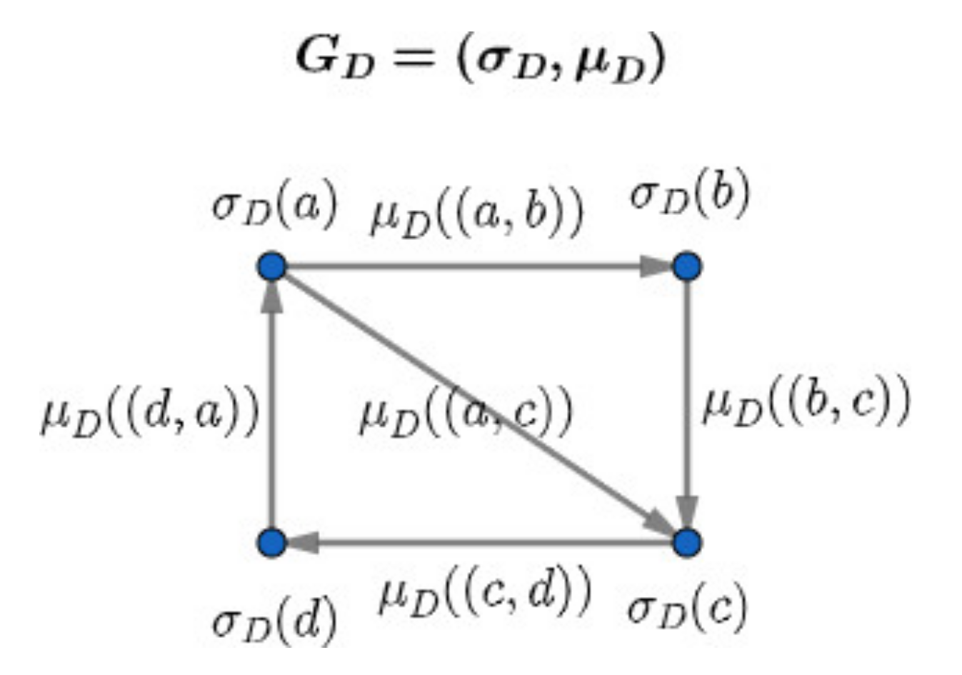
Definition 1.

Let  $G_D^{*}=\left(V,A\right)$ be a directed simple graph, where $V$ is a finite nonempty set and $A=\left\{\left(x,y\right):x,y\in V,x\ne y\right\}$. A fuzzy digraph $G_D=\left({\sigma }_D,{\mu }_D\right)$ is a pair of two functions ${\sigma }_D:V\to \left[0,1\right]$ and ${\mu }_D:A\to \left[0,1\right]$ such that ${\mu }_D\left(\left(x,y\right)\right)\le {\sigma }_D\left(x\right)\wedge {\sigma }_D\left(y\right)$ for all $x,y\in V$.

Remark 1.

The$G_D^{*}=\left(V,A\right)$is called a latent (hidden) directed graph of$G_D=\left({\sigma }_D,{\mu }_D\right)$. The term digraph is used to represent a directed graph.

Remark 2.

Let$G_D^{*}$be a latent digraph of$G_D$.

1. 

$V$is a set of vertices or nodes of a latent digraph, that is,

$$V=\left\{x:x is a vertex or node of G_D^{*}\right\}$$

2. 

$A$is a set of directed edges or arcs of a latent digraph, that is,

$$A=\left\{\left(x,y\right):x,y\in V,x\ne y\right\}$$

3. 

${\sigma }_D$is a set of vertices or nodes of a fuzzy digraph, that is,

$${\sigma }_D=\left\{{\sigma }_D\left(x\right):x\in V\right\}$$

4. 

${\mu }_D$is a set of edges or arcs of a fuzzy digraph, that is,

$${\mu }_D=\left\{{\mu }_D\left(\left(x,y\right)\right):x,y\in V\right\}$$

5. 

${\mu }_D\left(\left(x,y\right)\right)$means the edge or arc is directed from${\sigma }_D\left(x\right)$to${\sigma }_D\left(y\right)$.

6. 

${\mu }_D\left(\left(x,y\right)\right)=0$if$\left(x,y\right)\cancel{\in }A$.

Example 1.

Consider a directed graph  $G_D^{*}=\left(V,A\right)$ such that $V=\left\{a,b,c,d\right\}$ and $A=\left\{\left(a,b\right),\left(b,c\right),\left(c,d\right),\left(d,a\right),\left(a,c\right)\right\}$. See Figure 1.

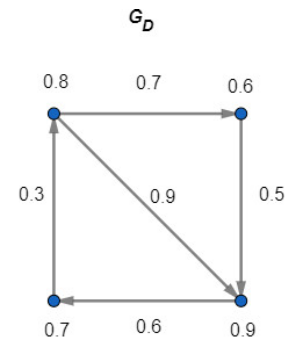
Example 2.

Let  $G_D=\left({\sigma }_D,{\mu }_D\right)$ and ${\mu }_D\left(u,v\right)\le {\sigma }_D\left(u\right)\wedge {\sigma }_D\left(v\right)$ for all $u,v\in V$ such that

${\sigma }_D=\left\{{\sigma }_D\left(a\right),{\sigma }_D\left(b\right),{\sigma }_D\left(c\right),{\sigma }_D\left(d\right)\right\}$and

${\mu }_D=\left\{{\mu }_D\left(\left(a,b\right)\right),{\mu }_D\left(\left(b,c\right)\right),{\mu }_D\left(\left(c,d\right)\right),{\mu }_D\left(\left(d,a\right)\right),{\mu }_D\left(\left(a,c\right)\right)\right\}$. See Figure 2.

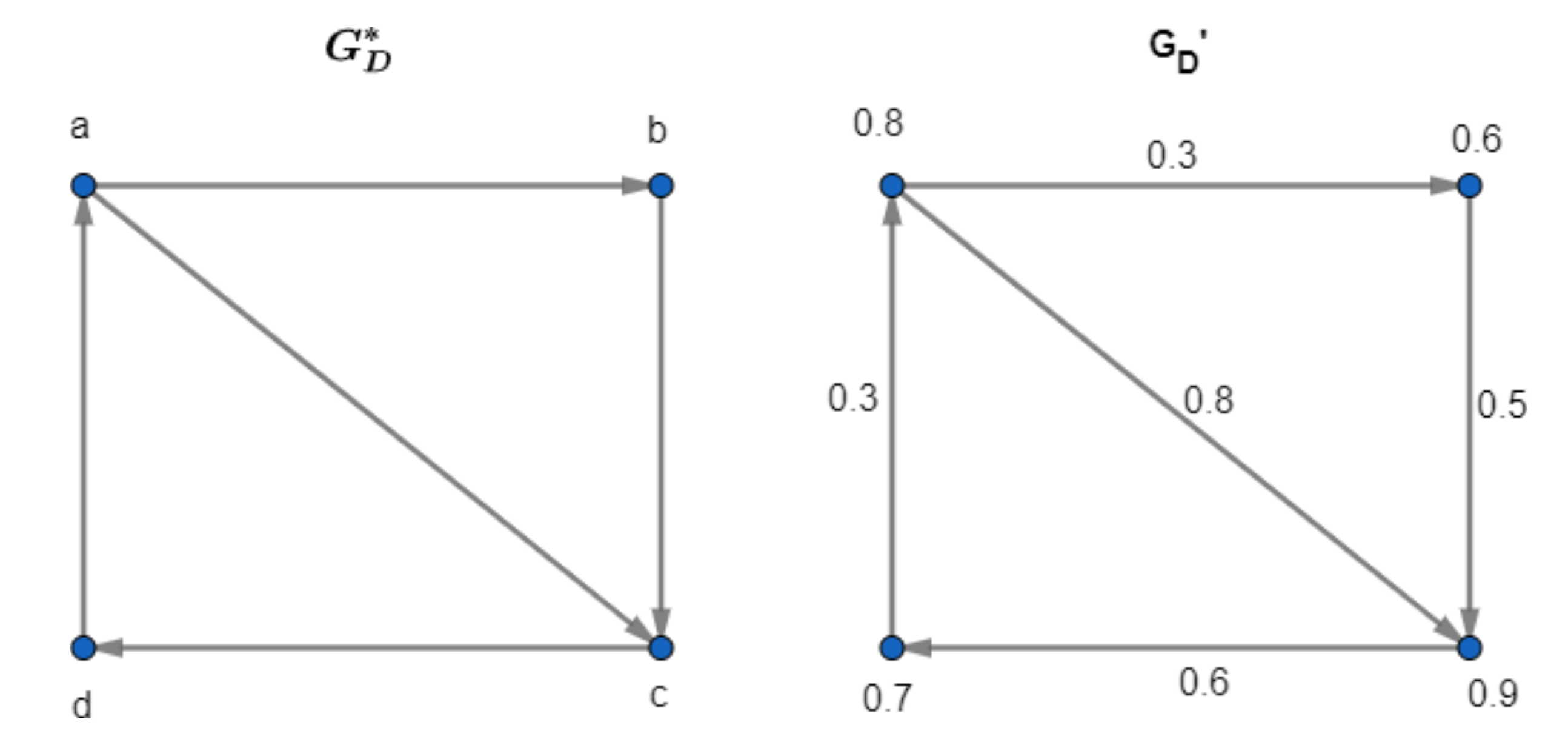
Example 3.

Let$G_D$be a directed graph as shown in Figure 3. Then,$G_D$is not a fuzzy digraph because$0.7\nleqq 0.8\wedge 0.6$. Moreover,$0.9\nleqq 0.8\wedge 0.9$.

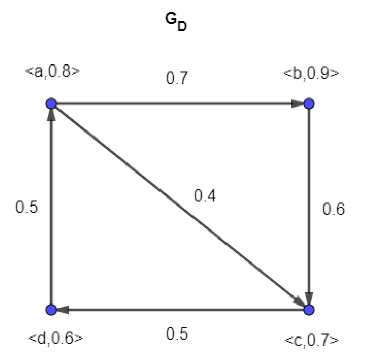
Example 4.

Let  $G_D^{*}=\left(V,A\right)$ be a latent digraph of $G_{D^{\prime }}$ as shown in Figure 4. Because ${\mu }_D\left(\left(x,y\right)\right)\le {\sigma }_D\left(x\right)\wedge {\sigma }_D\left(y\right)$ for all $x,y\in V$, it follows that $G_{D^{\prime }}$ is a fuzzy digraph.

Definition 2.

Let  $G_D^{*}=\left(V,A\right)$ be a latent digraph of $G_D$. The order $p$ and size $q$ of a fuzzy digraph $G_D=\left({\sigma }_D,{\mu }_D\right)$ are defined to b

$$p={{\displaystyle \sum }}_{x\in V}{\sigma }_D\left(x\right) and q={{\displaystyle \sum }}_{\left(x,y\right)\in A}{\mu }_D\left(\left(x,y\right)\right) for all x,y\in V$$

Example 5.

In Figure 4, the order$p$of$G_D^{\prime }$is

$$\begin{array}{l}p={\displaystyle \sum _{x\in V}}{\sigma }_D\left(x\right)\\ ={\sigma }_D\left(a\right)+{\sigma }_D\left(b\right)+{\sigma }_D\left(c\right)+{\sigma }_D\left(d\right)\\ =0.8+0.6+0.9+0.7\\ =3.0\end{array}$$

 and the size$q$of$G_D^{\prime }$ is

$$\begin{array}{l}q={{\displaystyle \sum }}_{\left(x,y\right)\in A}{\mu }_D\left(\left(x,y\right)\right)\\ ={\mu }_D\left(a,b\right)+{\mu }_D\left(b,c\right)+{\mu }_D\left(c,d\right)+{\mu }_D\left(d,a\right)+{\mu }_D\left(a,c\right)\\ =0.3+0.5+0.6+0.3+0.8=2.5\end{array}$$

Definition 3.

An arc  ${\mu }_D\left(\left(x,y\right)\right)$ of a fuzzy digraph is called an effective arc if

$${\mu }_D\left(\left(x,y\right)\right)={\sigma }_D\left(x\right)\wedge {\sigma }_D\left(y\right)$$

Example 6.

In Figure 4,${\mu }_D\left(\left(a,c\right)\right)=0.8$is the only effective arc of$G_D^{\prime }$.

3. Domination in Fuzzy Digraphs

In this section, we define a dominating set in a fuzzy digraph $G_D$. Further, we characterize the minimal dominating set of a fuzzy digraph and give some useful results.

Definition 4.

Let  $x,y\in V$. The vertex ${\sigma }_D\left(x\right)$ dominates ${\sigma }_D\left(y\right)$ in $G_D$ if ${\mu }_D\left(\left(x,y\right)\right)$ is an effective arc.

Example 7.

In Figure 4, as  ${\mu }_D\left(\left(a,c\right)\right)=0.8$ is an effective arc of $G_D^{\prime }$, ${\sigma }_D\left(a\right)=0.8$ dominates ${\sigma }_D\left(c\right)=0.9$.

Definition 5.

Let  $S\subseteq V$, $u\in V\backslash S$, and $v\in S$. A subset ${\sigma }_D\left(S\right)\subseteq {\sigma }_D$ is a dominating set of $G_D$ if, for every ${\sigma }_D\left(u\right)\in {\sigma }_D\backslash {\sigma }_D\left(S\right)$, there exists ${\sigma }_D\left(v\right)\in {\sigma }_D\left(S\right)$ such that ${\sigma }_D\left(v\right)$ dominates ${\sigma }_D\left(u\right)$.

Remark 3.

Let  $G_D=\left({\sigma }_D,{\mu }_D\right)$ be a fuzzy digraph of $G_D^{*}=\left(V,A\right)$ and $S\subseteq V$.

1. 

Then

$${\sigma }_D\left(S\right)=\left\{{\sigma }_D\left(x\right):x\in S\right\}$$

2. 

If${\sigma }_D\left(S\right)$is a dominating set of$G_D$, then$S$is a dominating set of$G_D^{*}$. The converse is not necessarily true.

3. 

The fuzzy cardinality of a minimum dominating set is called the domination number of$G_D$and is denoted by$\gamma \left(G_D\right)$, that is,

$$\gamma \left(G_D\right)=\min {{\displaystyle \sum }}_{x\in S}{\sigma }_D\left(x\right)$$

where$S$is a dominating set of$G_D^{*}.$

Remark 4.

Let  $G_D^{*}=\left(V,A\right)$ be a latent directed graph of a fuzzy digraph $G_D=\left({\sigma }_D,{\mu }_D\right)$. If ${\mu }_D\left(x,y\right)<{\sigma }_D\left(x\right)\wedge {\sigma }_D\left(y\right)$ for all $x,y\in V$ , then the only dominating set of $G_D$ is ${\sigma }_D$.

Example 8.

Let  $G_D^{*}=\left(V=\left\{a,b,c,d\right\},A\right)$ be a latent directed graph of a fuzzy digraph $G_D$ as shown in Figure 5. Because ${\mu }_D\left(x,y\right)<{\sigma }_D\left(x\right)\wedge {\sigma }_D\left(y\right)$ for all $x,y\in V$, the only dominating set of $G_D$ is ${\sigma }_D=\left\{0.8,0.9,0.7,0.6\right\}$. Hence, $\gamma \left(G_D\right)=3.0$.

Example 9.

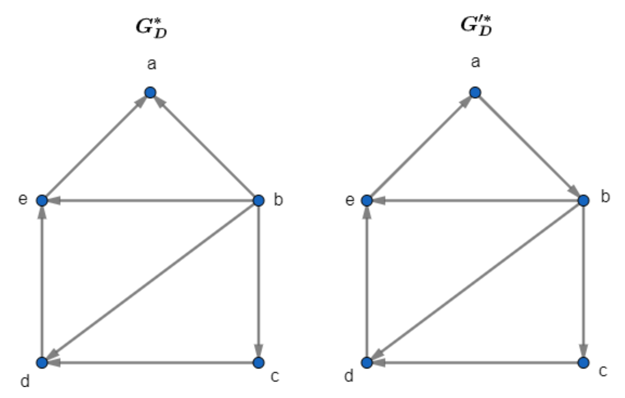
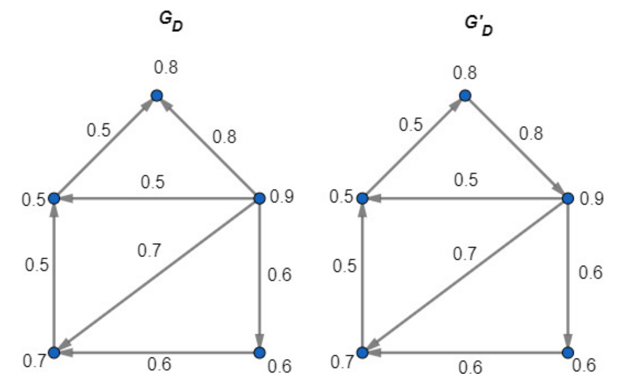
Let  $G_D^{*}$ and $G_{D^{\prime }}^{*}$ be latent digraphs of fuzzy digraphs $G_D=\left({\sigma }_D,{\mu }_D\right)$ and $G_{D\prime }=\left({\sigma }_{D^{\prime }},{\mu }_{D^{\prime }}\right)$, respectively (see Figure 6). If

$$\begin{gathered} {\sigma }_D=\left\{\frac{a}{0.8},\frac{b}{0.9},\frac{c}{0.6},\frac{d}{0.7},\frac{e}{0.5}\right\}={\sigma }_{D^{\prime }} \\ {\mu }_D=\left\{ba/0.8,bc/0.6,bd/0.7,be/0.5,cd/0.6,de/0.5,ea/0.5\right\}, \end{gathered}$$

and

$${\mu }_{D^{\prime }}=\left\{ab/0.8,bc/0.6,bd/0.7,be/0.5,cd/0.6,de/0.5,ea/0.5\right\}$$

then ${\mu }_D\left(\left(x,y\right)\right)={\sigma }_D\left(x\right)\wedge {\sigma }_D\left(y\right)$ for all $x,y\in V$. Hence, the set $\left\{0.9\right\}$ is the minimal dominating set of $G_D$ and the sets $\left\{0.8,0.9\right\}$, $\left\{0.5,0.9\right\}$, and $\left\{0.5,0.6,0.8\right\}$ are minimal dominating sets of $G_{D^{\prime }}$. Further, the domination number of $G_D$ is $\gamma \left(G_D\right)=0.9$ and the domination number of $G_{D\prime }$ is $\gamma \left(G_{D^{\prime }}\right)=1.4$ (see Figure 7).

From the definitions and observations, the following remark is immediate.

Remark 5.

Let  $G_D^{*}=\left(V,A\right)$ be a latent directed graph of a fuzzy digraph $G_D=\left({\sigma }_D,{\mu }_D\right)$. If $S\subseteq V$, then ${\displaystyle \sum }_{x\in S}{\sigma }_D\left(x\right)\le \left|S\right|.$

Proof. 

Because $0\le {\sigma }_D\left(x\right)\le 1$ for all $x\in S$, it follows that

$${{\displaystyle \sum }}_{x\in S}{\sigma }_D\left(x\right)\le {{\displaystyle \sum }}_{x\in S}1={{\displaystyle \sum }}_{n=1}^{\left|S\right|}1=1\left|S\right|=\left|S\right|.$$

□

The following result gives a characterization of the minimal dominating set of a fuzzy directed graph.

Theorem 1.

Let  $G_D^{*}=\left(V,A\right)$ be a latent directed graph of a fuzzy digraph $G_D=\left({\sigma }_D,{\mu }_D\right)$ and $S\subseteq V$. A dominating set ${\sigma }_D\left(S\right)$ of $G_D$ is minimal if and only if, for each ${\sigma }_D\left(x\right)\in {\sigma }_D\left(S\right)$, either $N_{G_D}\left({\sigma }_D\left(x\right)\right)\cap {\sigma }_D\left(S\right)=⌀$ or $N_{G_D}\left({\sigma }_D\left(y\right)\right)\cap {\sigma }_D\left(S\right)=\left\{{\sigma }_D\left(x\right)\right\}$ for some ${\sigma }_D\left(y\right)\in {\sigma }_D\backslash {\sigma }_D\left(S\right)$.

Proof. 

Let ${\sigma }_D\left(x\right)\in {\sigma }_D\left(S\right)$. If ${\sigma }_D\left(S\right)$ is a minimal dominating set of $G_D$, then ${\sigma }_D\left(S\right)\backslash {\sigma }_D\left(x\right)$ is not a dominating set of $G_D$. Thus, there exists ${\sigma }_D\left(y\right)\notin \left({\sigma }_D\left(S\right)\backslash {\sigma }_D\left(x\right)\right)$ such that ${\sigma }_D\left(y\right)$ is not dominated by any element of ${\sigma }_D\left(S\right)\backslash {\sigma }_D\left(x\right)$.

Case 1. Suppose ${\sigma }_D\left(y\right)={\sigma }_D\left(x\right)$. Then, ${\sigma }_D\left(x\right)$ is not dominated by any element of ${\sigma }_D\left(S\right)\backslash {\sigma }_D\left(x\right)$, that is, $N_{G_D}\left({\sigma }_D\left(x\right)\right)\cap {\sigma }_D\left(S\right)=⌀$.

Case 2. Suppose ${\sigma }_D\left(y\right)\ne {\sigma }_D\left(x\right)$. Then, ${\sigma }_D\left(y\right)\notin {\sigma }_D\left(S\right)$. Because ${\sigma }_D\left(S\right)$ is a minimum dominating set of $G_D$, it follows that ${\sigma }_D\left(y\right)$ is dominated by ${\sigma }_D\left(x\right)\in {\sigma }_D\left(S\right)$. Thus, $N_{G_D}\left({\sigma }_D\left(y\right)\right)\cap {\sigma }_D\left(S\right)=\left\{{\sigma }_D\left(x\right)\right\}$ for some ${\sigma }_D\left(y\right)\in {\sigma }_D\backslash {\sigma }_D\left(S\right)$.

For the converse, the proof is immediate. □

4. Some Special Fuzzy Digraphs

In this section, we introduce the definition of some special fuzzy digraphs $G_D$. Further, we give the general formula of computing the domination number of $G_D$.

Definition 6.

A fuzzy dipath (directed path)  $P_{{\sigma }_D}$ is a sequence of effective arcs having the property that the ending vertex of each arc is the same as the starting vertex of the next arc in the sequence.

Remark 6.

Let$P_{{\sigma }_D}=\left({\sigma }_D,{\mu }_D\right)$be a fuzzy dipath of a latent directed path$P_n=\left(V,A\right)$where$n\ge 2$is an integer. Then,

1. 

${\sigma }_D=\left\{{\sigma }_D\left(x_i\right):x_i\in V for all i\in \left\{1,2,\dots ,n\right\}\right\}$;

2. 

${\mu }_D=\left\{{\mu }_D\left(x_i,x_{i+1}\right):\left(x_i,x_{i+1}\right)\in A for all i\in \left\{1,2,\dots ,\left(n-1\right)\right\}\right\}$;

3. 

${\mu }_D\left(x_i,x_{i+1}\right)=\left({\sigma }_D\left(x_i\right),{\sigma }_D\left(x_{i+1}\right)\right) for all i\in \left\{1,2,\dots ,\left(n-1\right)\right\}$.

4. 

The vertices${\sigma }_D\left(x_1\right)$and${\sigma }_D\left(x_n\right)$are the first and last vertex, respectively, of a nontrivial fuzzy dipath.

The following result illustrates the domination number of a fuzzy dipath.

Theorem 2.

Let  $P_{{\sigma }_D}$ be a fuzzy dipath. Then, one of the following is satisfied.

1. 

$\gamma \left(P_{{\sigma }_D}\right)={{\displaystyle \sum }}_{k=1}^{n/2}{\sigma }_D\left(x_{2k-1}\right);$

2. 

$\gamma \left(P_{{\sigma }_D}\right)=\min X$, where

$$X=\left\{{{\displaystyle \sum }}_{k=1}^{\left(n+1\right)/2-i}{\sigma }_D\left(x_{2k-1}\right)+{{\displaystyle \sum }}_{k=\left(n+3\right)/2-i}^{\left(n+1\right)/2}{\sigma }_D\left(x_{2k-2}\right):i\in \left\{0,1,2,\dots ,\left(n-1\right)/2\right\}\right\}$$

Proof. 

By Remark 6, ${\sigma }_D=\left\{{\sigma }_D\left(x_i\right):x_i\in V,\forall i\in \left\{1,2,\dots ,n\right\}\right\}$ and

$${\mu }_D=\left\{{\mu }_D\left(x_i,x_{i+1}\right):\left(x_i,x_{i+1}\right)\in A,\forall i\in \left\{1,2,\dots ,\left(n-1\right)\right\}\right\}.$$

Because ${\mu }_D\left(x_i,x_{i+1}\right)$ is an effective arc for all $i\in \left\{1,2,\dots ,\left(n-1\right)\right\}$, it follows that ${\sigma }_D\left(x_i\right)$ dominate ${\sigma }_D\left(x_{i+1}\right)$ for all $i\in \left\{1,2,\dots ,\left(n-1\right)\right\}$.

Case 1. If $n$ is an even integer, then $n=2k$ for some positive integer $k$. Now, the set $\left\{{\sigma }_D\left(x_1\right),{\sigma }_D\left(x_3\right),\dots ,{\sigma }_D\left(x_{n-1}\right)\right\}$ is clearly the minimum dominating set of $P_{{\sigma }_D}$. Note that

$${\sigma }_D\left(x_1\right),{\sigma }_D\left(x_3\right),\dots ,{\sigma }_D\left(x_{n-1}\right)={{\displaystyle \sum }}_{k=1}^{n/2}{\sigma }_D\left(x_{2k-1}\right).$$

Thus, $\gamma \left(P_{\sigma D}\right)={{\displaystyle \sum }}_{k=1}^{n/2}{\sigma }_D\left(x_{2k-1}\right).$ This proves the statement $\left(i\right)$.

Case 2. If $n$ is an odd integer, then $n=2k-1$ for some positive integer $k$. Now, the sets

$$\begin{gathered} \left\{{\sigma }_D\left(x_1\right),{\sigma }_D\left(x_3\right),\dots ,{\sigma }_D\left(x_n\right)\right\}, \\ \left\{{\sigma }_D\left(x_1\right),{\sigma }_D\left(x_3\right),\dots ,{\sigma }_D\left(x_{n-2}\right),{\sigma }_D\left(x_{n-1}\right)\right\}, \\ \left\{{\sigma }_D\left(x_1\right),{\sigma }_D\left(x_3\right),\dots ,{\sigma }_D\left(x_{n-4}\right),{\sigma }_D\left(x_{n-3}\right),{\sigma }_D\left(x_{n-1}\right)\right\}, \\ \dots ,\left\{{\sigma }_D\left(x_1\right),{\sigma }_D\left(x_2\right),\dots ,{\sigma }_D\left(x_{n-5}\right),{\sigma }_D\left(x_{n-3}\right),{\sigma }_D\left(x_{n-1}\right)\right\} \end{gathered}$$

are minimal dominating sets of $P_{{\sigma }_D}$. Note that

$${\sigma }_D\left(x_1\right)+{\sigma }_D\left(x_3\right)+\dots +{\sigma }_D\left(x_n\right)={{\displaystyle \sum }}_{k=1}^{\left(n+1\right)/2}{\sigma }_D\left(x_{2k-1}\right).$$

Generally,

$$\begin{gathered} {\sigma }_D\left(x_1\right)+{\sigma }_D\left(x_3\right)+\dots +{\sigma }_D\left(x_j\right)+{\sigma }_D\left(x_{j+1}\right)+\dots +{\sigma }_D\left(x_{n-3}\right)+{\sigma }_D\left(x_{n-1}\right) \\ ={\displaystyle \sum }_{k=1}^{\left(j+1\right)/2}{\sigma }_D\left(x_{2k-1}\right)+{\displaystyle \sum }_{k=\left(j+3\right)/2}^{\left(n+1\right)/2}{\sigma }_D\left(x_{2k-2}\right). \end{gathered}$$

Let $\left(j+1\right)/2+i=\left(n+1\right)/2$ for $i\in \left\{0,1,2,\dots ,\left(n-1\right)/2\right\}$. Then

$${{\displaystyle \sum }}_{k=1}^{\left(n+1\right)/2-i}{\sigma }_D\left(x_{2k-1}\right)+{{\displaystyle \sum }}_{k=\left(n+3\right)/2-i}^{\left(n+1\right)/2}{\sigma }_D\left(x_{2k-2}\right).$$

Thus, the minimum of

$$X=\left\{{{\displaystyle \sum }}_{k=1}^{\left(n+1\right)/2-i}{\sigma }_D\left(x_{2k-1}\right)+{{\displaystyle \sum }}_{k=\left(n+3\right)/2-i}^{\left(n+1\right)/2}{\sigma }_D\left(x_{2k-2}\right):i\in \left\{0,1,2,\dots ,\left(n-1\right)/2\right\}\right\}$$

is the domination number of a fuzzy dipath $P_{{\sigma }_D}$. Hence, $\gamma \left(P_{{\sigma }_D}\right)=\min X$. □

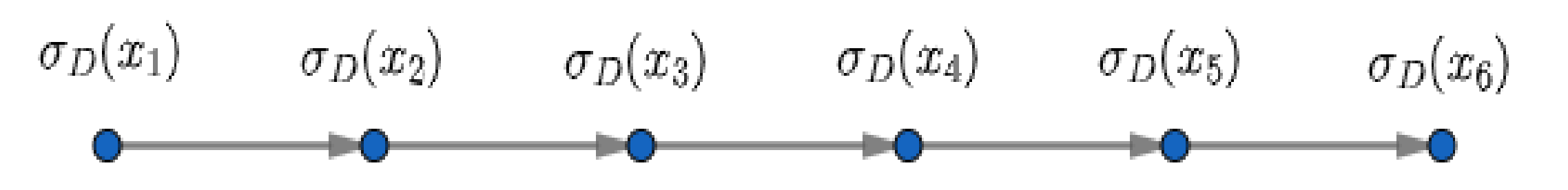
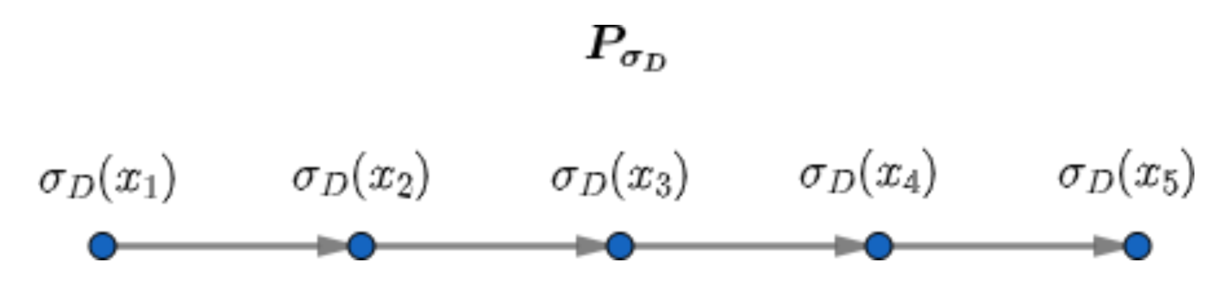
Example 10.

Let $P_{{\sigma }_D}=\left({\sigma }_D,{\mu }_D\right)$ be a fuzzy dipath of a latent directed path $P_6=\left(V,A\right)$. (see Figure 8).

Example 11.

Let$P_{{\sigma }_D}=\left({\sigma }_D,{\mu }_D\right)$be a fuzzy dipath of a latent directed path$P_5=\left(V,A\right)$. Let$X=\left\{{\sigma }_D\left(x_1\right),{\sigma }_D\left(x_3\right),{\sigma }_D\left(x_5\right)\right\}$, $Y=\left\{{\sigma }_D\left(x_1\right),{\sigma }_D\left(x_3\right),{\sigma }_D\left(x_4\right)\right\}$, and$Z=\left\{{\sigma }_D\left(x_1\right),{\sigma }_D\left(x_2\right),{\sigma }_D\left(x_4\right)\right\}$(see Figure 9).

Corollary 1.

Let  $P_{{\sigma }_D}=\left({\sigma }_D,{\mu }_D\right)$ be a fuzzy dipath of a latent nontrivial directed path $P_n=\left(V,A\right)$. If ${\sigma }_D\left(x\right)={\sigma }_D\left(y\right)$, $\forall x,y\in V$, then $\lceil \frac{n}{2}\rceil {\sigma }_D\left(x\right)$.

Proof. 

If $n$ is even, by Theorem 2, $\gamma \left(P_{{\sigma }_D}\right)={{\displaystyle \sum }}_{k=1}^{n/2}{\sigma }_D\left(x_{2k-1}\right)$. Because ${\sigma }_D\left(x\right)={\sigma }_D\left(y\right)$, $\forall x,y\in V$, it follows that ${\sigma }_D\left(x_1\right)={\sigma }_D\left(x_3\right)=\dots ={\sigma }_D\left(x_{n-1}\right)={\sigma }_D\left(x\right)$. Thus,

$$\gamma \left(P_{{\sigma }_D}\right)={{\displaystyle \sum }}_{k=1}^{n/2}{\sigma }_D\left(x\right)=\left(\frac{n}{2}\right){\sigma }_D\left(x\right).$$

Similarly, if $n$ is odd, by Theorem 2,

$$\begin{array}{l}\gamma \left(P_{{\sigma }_D}\right)={\displaystyle \sum }_{k=1}^{\left(n+1\right)/2-i}{\sigma }_D\left(x_{2k-1}\right)+{\displaystyle \sum }_{k=\left(n+3\right)/2-i}^{\left(n+1\right)/2}{\sigma }_D\left(x_{2k-2}\right)for i\in \{0,1,2,\dots ,\left(n-1\right)/2\\ ={\displaystyle \sum }_{k=1}^{\left(n+1\right)/2-i}{\sigma }_D\left(x\right)+{\displaystyle \sum }_{k=\left(n+3\right)/2-i}^{\left(n+1\right)/2}{\sigma }_D\left(x\right)\\ =\left(\left(n+1\right)/2-i\right){\sigma }_D\left(x\right)+\left[\left(n+1\right)/2-\left(\left(n+3\right)/2-i+1\right)\right]{\sigma }_D\left(x\right)\\ =\left(\frac{n+1}{2}\right){\sigma }_D\left(x\right).\end{array}$$

Hence, $\gamma \left(P_{{\sigma }_D}\right)$ is either $\left(\frac{n}{2}\right){\sigma }_D\left(x\right)$ if n is even, or $\left(\frac{n+1}{2}\right){\sigma }_D\left(x\right)$ if n is odd. Therefore, $\gamma \left(P_{{\sigma }_D}\right)=\lceil \frac{n}{2}\rceil {\sigma }_D\left(x\right).$ □

Definition 7.

A fuzzy dicycle (directed cycle)  $C_{{\sigma }_D}$ is a dipath where it starts and ends with the same vertex.

Remark 7.

Let  $C_{{\sigma }_D}=\left({\sigma }_D,{\mu }_D\right)$ be a fuzzy dicycle of a latent directed cycle $C_n=\left(V,A\right)$, where $n\ge 3$. Then,

1. 

${\sigma }_D=\left\{{\sigma }_D\left(x_i\right):x_i\in V,\forall i\in \left\{1,2,\dots ,n\right\}\right\}$;

2. 

${\mu }_D=\left\{{\mu }_D\left(x_i,x_{i+1}\right),{\mu }_D\left(x_n,x_1\right):\left(x_i,x_{i+1}\right),\left(x_n,x_1\right)\in A,\forall i\in \left\{1,2,\dots ,\left(n-1\right)\right\}\right\}$;

3. 

${\mu }_D\left(x_i,x_{i+1}\right)=\left({\sigma }_D\left(x_i\right),{\sigma }_D\left(x_{i+1}\right)\right),\forall i\in \left\{1,2,\dots ,\left(n-1\right)\right\}$.

The following result provides the domination number of a fuzzy dicycle.

Theorem 3.

Let$C_{{\sigma }_D}=\left({\sigma }_D,{\mu }_D\right)$be a fuzzy dicycle of a latent directed cycle$C_n=\left(V,A\right)$ where $n\ge 3$. Then, one of the following is satisfied:

1. 

$\gamma \left(C_{{\sigma }_D}\right)=min\left\{{{\displaystyle \sum }}_{k=1}^{n/2}{\sigma }_D\left(x_{2k-1}\right),{{\displaystyle \sum }}_{k=1}^{n/2}{\sigma }_D\left(x_{2k}\right)\right\}$;

2. 

$\gamma \left(C_{{\sigma }_D}\right)=min\left(X\cup Y\right)$, where

$$X=\left\{{{\displaystyle \sum }}_{k=1}^{\left(n+1\right)/2-i}{\sigma }_D\left(x_{2k-1}\right)+{{\displaystyle \sum }}_{k=\left(n+3\right)/2-i}^{\left(n+1\right)/2}{\sigma }_D\left(x_{2k-2}\right):i\in \left\{0,1,2,\dots ,\left(n-1\right)/2\right\}\right\},$$

$$Y=\left\{{{\displaystyle \sum }}_{k=1}^{\left(n+1\right)/2-i}{\sigma }_D\left(x_{2k}\right)+{{\displaystyle \sum }}_{k=\left(n+3\right)/2-i}^{\left(n+1\right)/2}{\sigma }_D\left(x_{2k-1}\right):i\in \left\{0,1,2,\dots ,\left(n-1\right)/2\right\}\right\}.$$

Proof. 

Let $I=\left\{1,2,\dots ,n\right\}$. Because $C_{{\sigma }_D}$ is a dipath that starts and ends with the same node, the arcs ${\mu }_D\left(x_i,x_{i+1}\right)$ for all $i\in I$ and ${\mu }_D\left(x_n,x_1\right)$ are effective. This means that ${\sigma }_D\left(x_i\right)$ dominate ${\sigma }_D\left(x_{i+1}\right)$ for all $i\in \left\{1,2,\dots ,n-1\right\}$ and ${\sigma }_D\left(x_n\right)$ dominate ${\sigma }_D\left(x_1\right)$.

Case 1. If $n$ is an even integer, then $n=2k$ for some positive integer $k$. Now, the sets $\left\{{\sigma }_D\left(x_1\right),{\sigma }_D\left(x_3\right),\dots ,{\sigma }_D\left(x_{n-1}\right)\right\}$ and $\left\{{\sigma }_D\left(x_2\right),{\sigma }_D\left(x_4\right),\dots ,{\sigma }_D\left(x_n\right)\right\}$ are minimal dominating sets of $C_{{\sigma }_D}$. Note that

$${\sigma }_D\left(x_1\right)+{\sigma }_D\left(x_3\right)+\dots +{\sigma }_D\left(x_{n-1}\right)={{\displaystyle \sum }}_{k=1}^{n/2}{\sigma }_D\left(x_{2k-1}\right)$$

and

$${\sigma }_D\left(x_2\right)+{\sigma }_D\left(x_4\right)+\dots +{\sigma }_D\left(x_n\right)={{\displaystyle \sum }}_{k=1}^{n/2}{\sigma }_D\left(x_{2k}\right)$$

Thus, $\gamma \left(C_{{\sigma }_D}\right)=\min \left\{{{\displaystyle \sum }}_{k=1}^{n/2}{\sigma }_D\left(x_{2k-1}\right),{{\displaystyle \sum }}_{k=1}^{n/2}{\sigma }_D\left(x_{2k}\right)\right\}.$ This proves the statement $\left(i\right)$.

Case 2. If $n$ is an odd integer, then $n=2k-1$ for some positive integer $k$. Now, the sets

$$\begin{gathered} \left\{{\sigma }_D\left(x_1\right),{\sigma }_D\left(x_3\right),\dots ,{\sigma }_D\left(x_n\right)\right\}, \\ \left\{{\sigma }_D\left(x_1\right),{\sigma }_D\left(x_3\right),\dots ,{\sigma }_D\left(x_{n-2}\right),{\sigma }_D\left(x_{n-1}\right)\right\}, \\ \left\{{\sigma }_D\left(x_1\right),{\sigma }_D\left(x_3\right),\dots ,{\sigma }_D\left(x_{n-4}\right),{\sigma }_D\left(x_{n-3}\right),{\sigma }_D\left(x_{n-1}\right)\right\}, \\ \dots ,\left\{{\sigma }_D\left(x_1\right),{\sigma }_D\left(x_2\right),\dots ,{\sigma }_D\left(x_{n-5}\right),{\sigma }_D\left(x_{n-3}\right),{\sigma }_D\left(x_{n-1}\right)\right\} \end{gathered}$$

are some minimal dominating sets of $C_{{\sigma }_D}$. Note that

$${\sigma }_D\left(x_1\right)+{\sigma }_D\left(x_3\right)+\dots +{\sigma }_D\left(x_n\right)={{\displaystyle \sum }}_{k=1}^{\left(n+1\right)/2}{\sigma }_D\left(x_{2k-1}\right).$$

Generally,

$$\begin{gathered} {\sigma }_D\left(x_1\right)+{\sigma }_D\left(x_3\right)+\dots +{\sigma }_D\left(x_j\right)+{\sigma }_D\left(x_{j+1}\right)+\dots +{\sigma }_D\left(x_{n-3}\right)+{\sigma }_D\left(x_{n-1}\right) \\ ={\displaystyle \sum }_{k=1}^{\left(j+1\right)/2}{\sigma }_D\left(x_{2k-1}\right)+{\displaystyle \sum }_{k=\left(j+3\right)/2}^{\left(n+1\right)/2}{\sigma }_D\left(x_{2k-2}\right). \end{gathered}$$

Let $\left(j+1\right)/2+i=\left(n+1\right)/2$. Then,

$${{\displaystyle \sum }}_{k=1}^{\left(n+1\right)/2-i}{\sigma }_D\left(x_{2k-1}\right)+{{\displaystyle \sum }}_{k=\left(n+3\right)/2-i}^{\left(n+1\right)/2}{\sigma }_D\left(x_{2k-2}\right),\forall i\in \left\{0,1,2,\dots ,\left(n-1\right)/2\right\}.$$

Further, the sets

$$\begin{gathered} \left\{{\sigma }_D\left(x_2\right),{\sigma }_D\left(x_4\right),\dots ,{\sigma }_D\left(n-1\right),{\sigma }_D\left(x_n\right)\right\}, \\ \left\{{\sigma }_D\left(x_2\right),{\sigma }_D\left(x_4\right),\dots ,{\sigma }_D\left(x_{n-3}\right),{\sigma }_D\left(x_{n-2}\right),{\sigma }_D\left(x_n\right)\right\}, \\ \left\{{\sigma }_D\left(x_2\right),{\sigma }_D\left(x_4\right),\dots ,{\sigma }_D\left(x_{n-5}\right),{\sigma }_D\left(x_{n-4}\right),{\sigma }_D\left(x_{n-2}\right),{\sigma }_D\left(x_n\right)\right\}, \\ \dots ,\left\{{\sigma }_D\left(x_2\right),{\sigma }_D\left(x_3\right),\dots ,{\sigma }_D\left(x_{n-4}\right),{\sigma }_D\left(x_{n-2}\right),{\sigma }_D\left(x_n\right)\right\} \end{gathered}$$

are other minimal dominating sets of $C_{{\sigma }_D}$. Generally,

$$\begin{gathered} {\sigma }_D\left(x_2\right)+{\sigma }_D\left(x_4\right)+\dots +{\sigma }_D\left(x_j\right)+{\sigma }_D\left(x_{j+1}\right)+\dots +{\sigma }_D\left(x_{n-2}\right)+{\sigma }_D\left(x_n\right) \\ ={\displaystyle \sum }_{k=1}^{j/2}{\sigma }_D\left(x_{2k}\right)+{\displaystyle \sum }_{k=\left(j+2\right)/2}^{\left(n+1\right)/2}{\sigma }_D\left(x_{2k-1}\right) \end{gathered}$$

Let $j/2+i=\left(n+1\right)/2$. Then,

$${{\displaystyle \sum }}_{k=1}^{\left(n+1\right)/2-i}{\sigma }_D\left(x_{2k}\right)+{{\displaystyle \sum }}_{k=\left(n+3\right)/2-i}^{\left(n+1\right)/2}{\sigma }_D\left(x_{2k-1}\right),\forall i\in \left\{0,1,2,\dots ,\left(n-1\right)/2\right\}$$

Let $I^{\prime }=\left\{0,1,2,\dots ,\left(n-1\right)/2\right\}$ such that

$$X=\left\{{{\displaystyle \sum }}_{k=1}^{\left(n+1\right)/2-i}{\sigma }_D\left(x_{2k-1}\right)+{{\displaystyle \sum }}_{k=\left(n+3\right)/2-i}^{\left(n+1\right)/2}{\sigma }_D\left(x_{2k-2}\right):\forall i\in I^{\prime }\right\}$$

and

$$Y=\left\{{{\displaystyle \sum }}_{k=1}^{\left(n+1\right)/2-i}{\sigma }_D\left(x_{2k}\right)+{{\displaystyle \sum }}_{k=\left(n+3\right)/2-i}^{\left(n+1\right)/2}{\sigma }_D\left(x_{2k-1}\right),\forall i\in I^{\prime }\right\}.$$

Hence, the domination number of $C_{{\sigma }_D}$ is $\gamma \left(C_{{\sigma }_D}\right)=\min \left(X{\displaystyle \cup }Y\right)$. This proves statement $ii)$ □

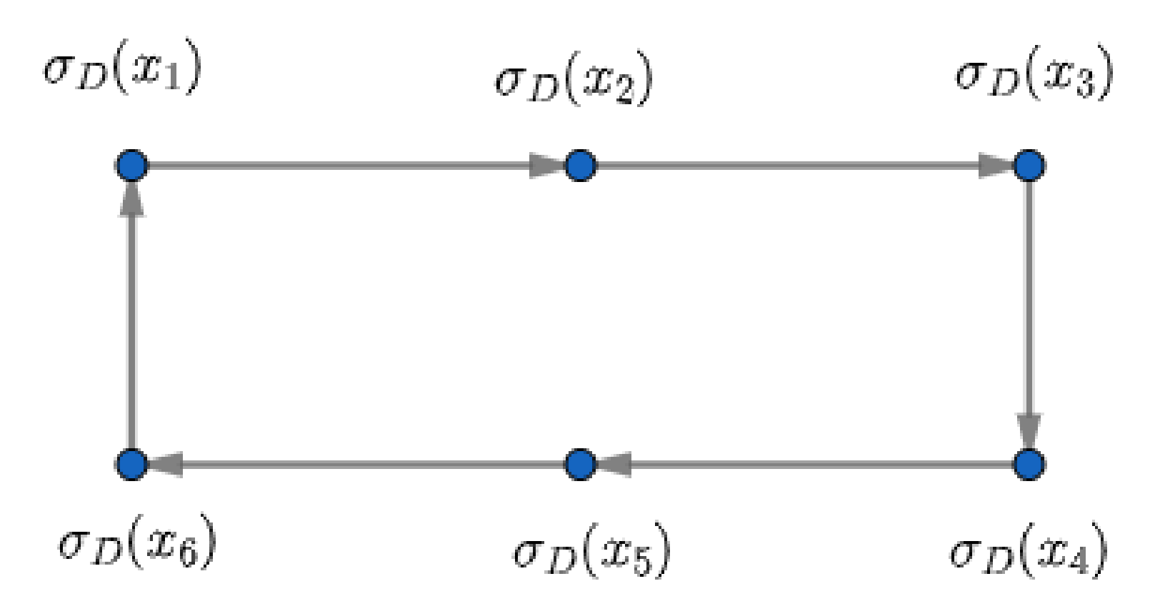
Example 12.

Let  $C_{{\sigma }_D}=\left({\sigma }_D,{\mu }_D\right)$ be a fuzzy dicycle of a latent directed cycle $C_5=\left(V,A\right)$. Let $X=\left\{{\sigma }_D\left(x_1\right),{\sigma }_D\left(x_3\right),{\sigma }_D\left(x_5\right)\right\}$ and $Y=\left\{{\sigma }_D\left(x_2\right),{\sigma }_D\left(x_4\right),{\sigma }_D\left(x_6\right)\right\}$ (see Figure 10).

Example 13.

Let  $C_{{\sigma }_D}=\left({\sigma }_D,{\mu }_D\right)$ be a fuzzy dicycle of a latent directed cycle  $C_5=\left(V,A\right)$. Let

$$\begin{gathered} X_1=\left\{{\sigma }_D\left(x_1\right),{\sigma }_D\left(x_3\right),{\sigma }_D\left(x_5\right)\right\} \\ {X}_2=\left\{{\sigma }_D\left(x_1\right),{\sigma }_D\left(x_2\right),{\sigma }_D\left(x_4\right)\right\},X_3=\left\{{\sigma }_D\left(x_2\right),{\sigma }_D\left(x_3\right),{\sigma }_D\left(x_5\right)\right\}, \\ {X}_4=\left\{{\sigma }_D\left(x_1\right),{\sigma }_D\left(x_3\right),{\sigma }_D\left(x_4\right)\right\},X_5=\left\{{\sigma }_D\left(x_2\right),{\sigma }_D\left(x_4\right),{\sigma }_D\left(x_5\right)\right\} \end{gathered}$$

(see Figure 11).

Corollary 2.

Let$C_{{\sigma }_D}=\left({\sigma }_D,{\mu }_D\right)$be a fuzzy dicycle of a latent directed cycle$C_n=\left(V,A\right)$where$n\ge 3$. If${\sigma }_D\left(x\right)={\sigma }_D\left(y\right)$,$\forall x,y\in V$, then$\lceil \frac{n}{2}\rceil {\sigma }_D\left(x\right)$.

Proof. 

If $n$ is even, by Theorem 3,

$$\gamma \left(C_{{\sigma }_D}\right)=\min \left\{{{\displaystyle \sum }}_{k=1}^{n/2}{\sigma }_D\left(x_{2k-1}\right),{{\displaystyle \sum }}_{k=1}^{n/2}{\sigma }_D\left(x_{2k}\right)\right\}.$$

Because ${\sigma }_D\left(x\right)={\sigma }_D\left(y\right)$, $\forall x,y\in V$, it is immediate that

$$\gamma \left(C_{{\sigma }_D}\right)={{\displaystyle \sum }}_{k=1}^{n/2}{\sigma }_D\left(x\right)=\left(\frac{n}{2}\right){\sigma }_D\left(x\right)$$

(using similar reasoning of Corollary 1.

Similarly, if $n$ is odd, by Theorem 3,

$$\begin{gathered} {{\displaystyle \sum }}_{k=1}^{\frac{n+1}{2}-i}{\sigma }_D\left(x_{2k-1}\right)+{{\displaystyle \sum }}_{k=\left(n+3\right)/2-i}^{\left(n+1\right)/2}{\sigma }_D\left(x_{2k-2}\right),\forall i\in \left\{0,1,2,\dots ,\left(n-1\right)/2\right\} \\ ={\displaystyle \sum _{k=1}^{\frac{n+1}{2}-i}}{\sigma }_D\left(x\right)+{\displaystyle {\displaystyle \sum }_{k=\left(n+3\right)/2-i}^{\left(n+1\right)/2}{\sigma }_D\left(x\right)} \end{gathered}$$

Because

$$\begin{array}{l}{\sigma }_D\left(x\right)={\sigma }_D\left(y\right), \forall x,y\in V,\\ =\left(\left(n+1\right)/2-i\right){\sigma }_D\left(x\right)+\left[\left(n+1\right)/2-\left(\left(n+3\right)/2-i+1\right)\right]{\sigma }_D\left(x\right)\\ =\left(\frac{n+1}{2}\right){\sigma }_D\left(x\right).\end{array}$$

and

$$\begin{array}{l}{{\displaystyle \sum }}_{k=1}^{\left(n+1\right)/2-i}{\sigma }_D\left(x_{2k}\right)+{{\displaystyle \sum }}_{k=\left(n+3\right)/2-i}^{\left(n+1\right)/2}{\sigma }_D\left(x_{2k-1}\right),\forall i\in \left\{0,1,2,\dots ,\left(n-1\right)/2\right\}\\ ={\displaystyle \sum _{k=1}^{\left(n+1\right)/2-i}}{\sigma }_D\left(x\right)+{\displaystyle \sum _{k=\left(n+3\right)/2-i}^{\left(n+1\right)/2}}{\sigma }_D\left(x\right), since {\sigma }_D\left(x\right)={\sigma }_D\left(y\right), \forall x,y\in V,\\ =\left(\frac{n+1}{2}\right){\sigma }_D\left(x\right).\end{array}$$

Hence, $\gamma \left(C_{{\sigma }_D}\right)$ is either $\left(\frac{n}{2}\right){\sigma }_D\left(x\right)$ if $n$ is even, or $\left(\frac{n+1}{2}\right){\sigma }_D\left(x\right)$ if n is odd.

Thus, $\gamma \left(C_{{\sigma }_D}\right)=\lceil \frac{n}{2}\rceil {\sigma }_D\left(x\right).$ □

5. Conclusions

In this work, we introduced the concept of domination in a fuzzy digraph, provided the characteristics of the minimum dominating set of fuzzy digraphs, and modeled the domination number of a fuzzy dipath and a fuzzy dicycle. The domination number in a fuzzy dipath and a fuzzy dicycle was presented and proved. The immediate consequences of the mentioned concepts were all proved. Some related problems are still open for future work.

(a)

Characterize the dominating sets of each of the following special fuzzy digraphs—the wheel $W_n$, the complete bipartite $K_{m,n}$, the star $S_n$, and the fan $F_n$.

(b)

Find the domination number of each of the following special fuzzy digraphs: $W_n$, $K_{m,n}$, $S_n$, and $F_n$.

Aside from these problems, future works could explore the application of domination in fuzzy digraphs in problem structuring methods commonly used in the literature, such as fuzzy decision-making trial and evaluation laboratory (DEMATEL) [29], fuzzy cognitive mapping (FCM) [30], and fuzzy interpretive structural modelling (ISM) [31], among others.