
Clustering of Latvian Pension Funds Using Convolutional Neural Network Extracted Features


Abstract
1. Introduction
2. Literature Review
2.1. Pension Funds
- The first pillar is a state-based pension scheme that emphasizes poverty prevention;
- Second-tier pension consists of occupational pension schemes that involve regular employer contributions and have a goal of ensuring adequate income;
- The third pillar is made of voluntary funded plans that supplement the income from the first two tiers.
- In DC-type plans, the employee decides where the money is invested, taking responsibility for the risks associated with investment and potential loss. A pensioner can outlive the investment, and it is not protected from inflation. Its return depends on the contributions made and investment performance.
- In the DB type of pension plans, the employer guarantees lifetime pension income regardless of funds’ performance, thus committing to covering the remainder of the underperforming fund. The plan provides lifetime income for retirees, which depends on the salary and years spent working. In addition, DB pension plans protect investment against inflation and are managed by pension fund supervisors.
2.2. Machine Learning Models and Their Application to the Real-World Tasks
2.3. The Application of Machine Learning in Pension Funds
3. Materials and Methods
3.1. Datasets and Preprocessing
- Column ID.
- Pension fund name.
- Date in force.
- Calculation date.
- NAV value in Latvian lats and euros.
- Amount of units.
- Total asset value in Latvian lats and euros.
- The number of participants.
3.2. Training the Neural Networks
3.2.1. Artificial Neural Networks
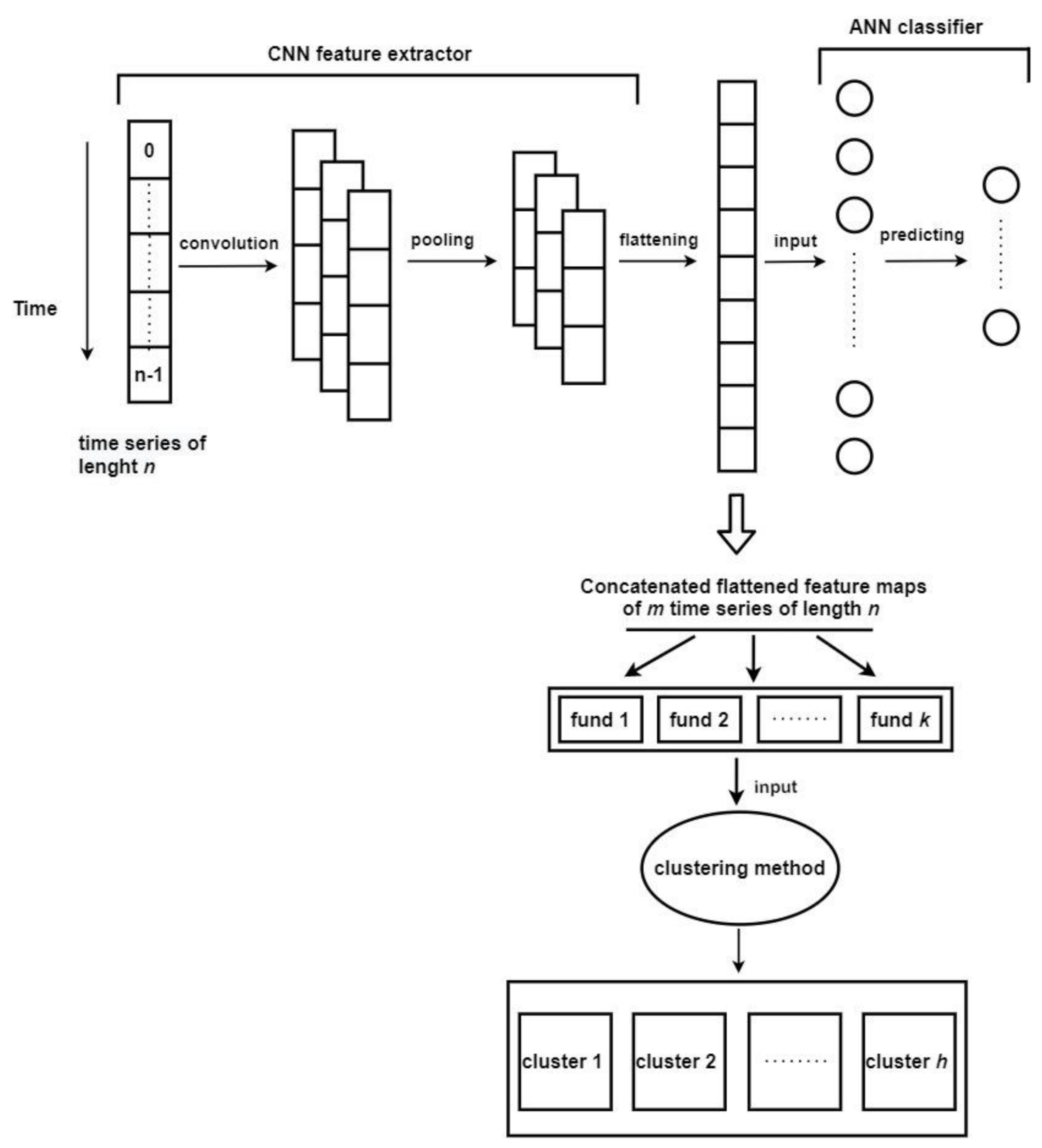
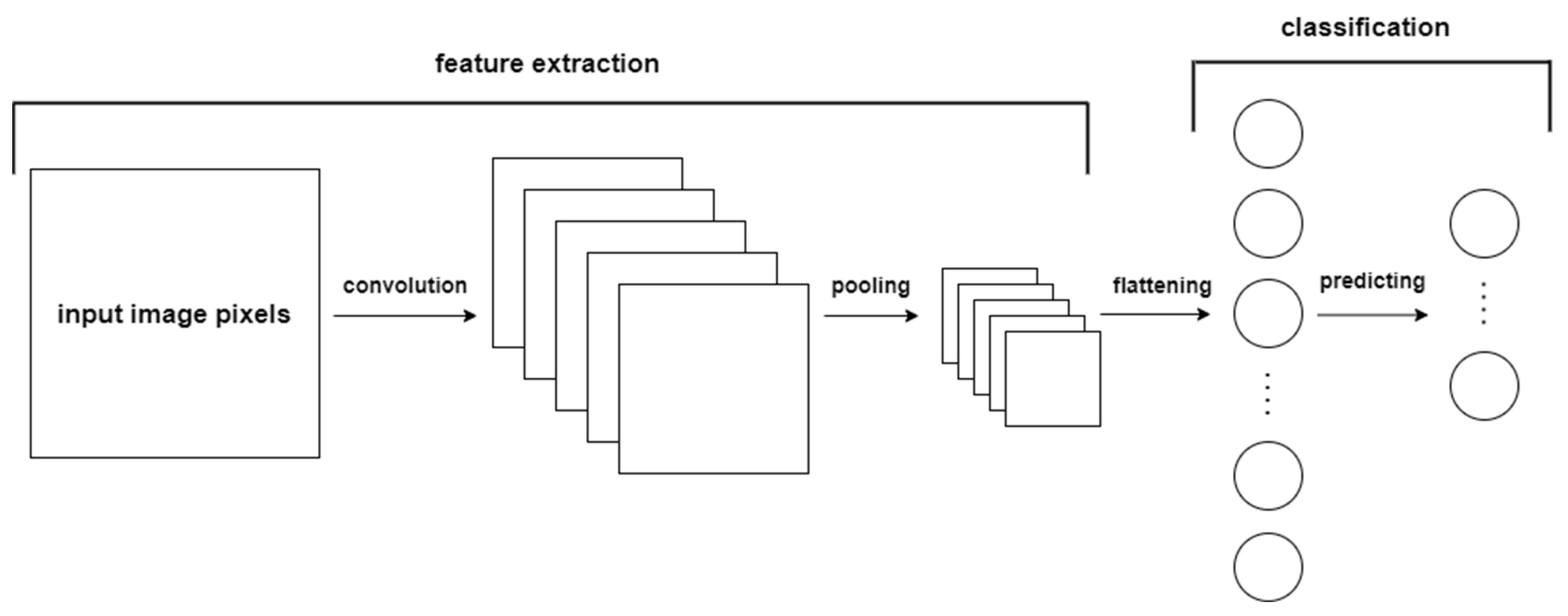
3.2.2. Convolutional Neural Networks
3.2.3. Classifier Performance Evaluation
- True positive (TP)—the model correctly predicted a positive label;
- False positive (FP)—the model predicted a positive label when the actual label was negative;
- True negative (TN)—the model correctly predicted a negative label;
- False negative (FN)—the model predicted a negative label when the actual label was positive.
3.3. Clustering
- Partition based: K-means, mini batch K-means;
- Hierarchy based: BIRCH, agglomerative clustering;
- Density based: DBSCAN, OPTICS, mean shift;
- Graph based: affinity propagation.
- Number of clusters—indicates to how many clusters the algorithm should group data;
- Random state—the seed to use for the pseudo-random number generator responsible for randomness;
- Min samples—the number of data points surrounding the point required to become a core of a cluster;
- Algorithm—the algorithm used for pointwise distance computation and nearest-neighbor calculation;
- Distance—the distance metric used by the algorithm.
3.3.1. Initial Clustering and Feature Extractor Performance
3.3.2. Pension Fund Clustering
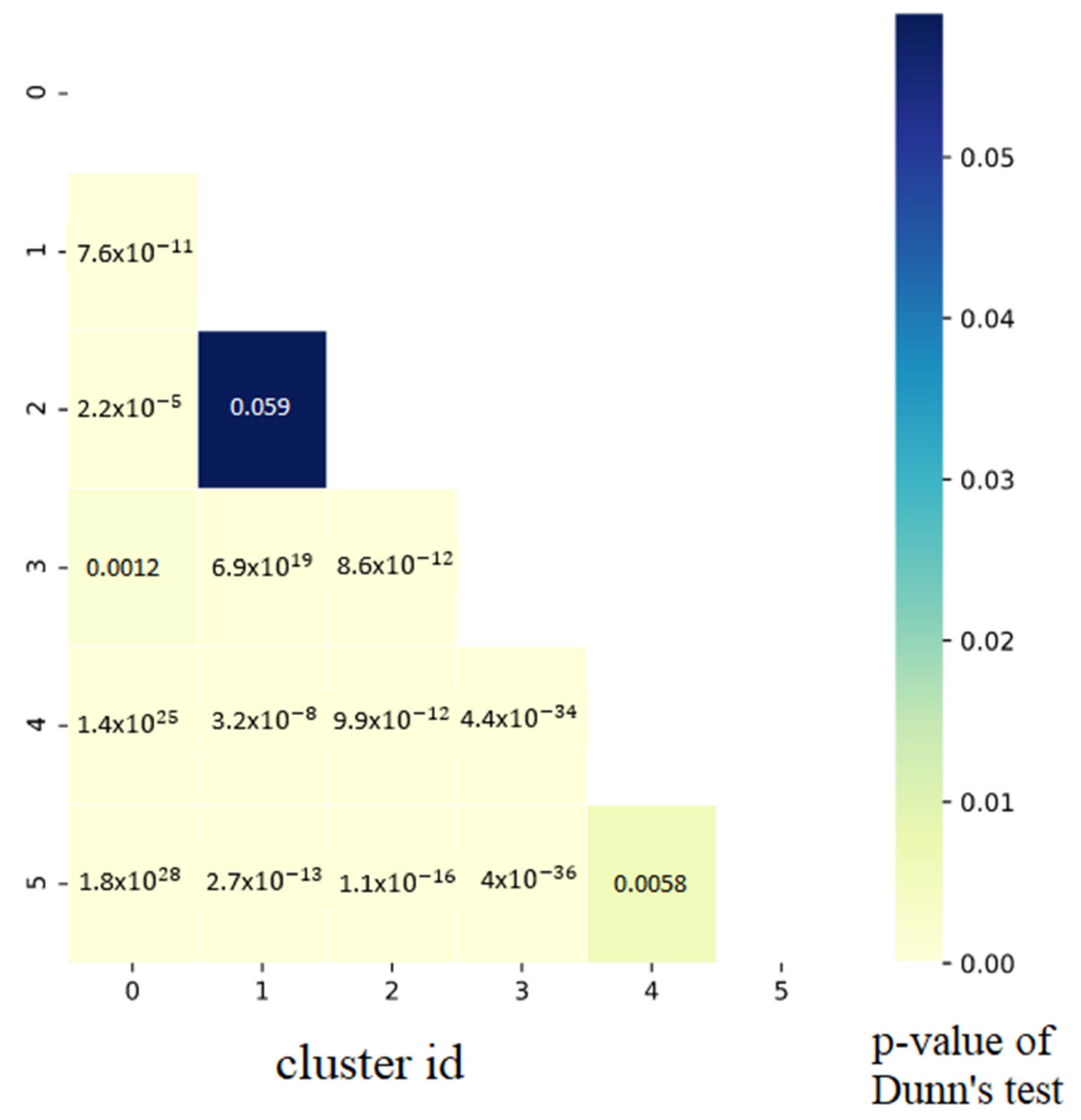
3.4. Post Hoc Testing
3.5. Summary of Research Methods
4. Results
4.1. Pension Fund Analysis
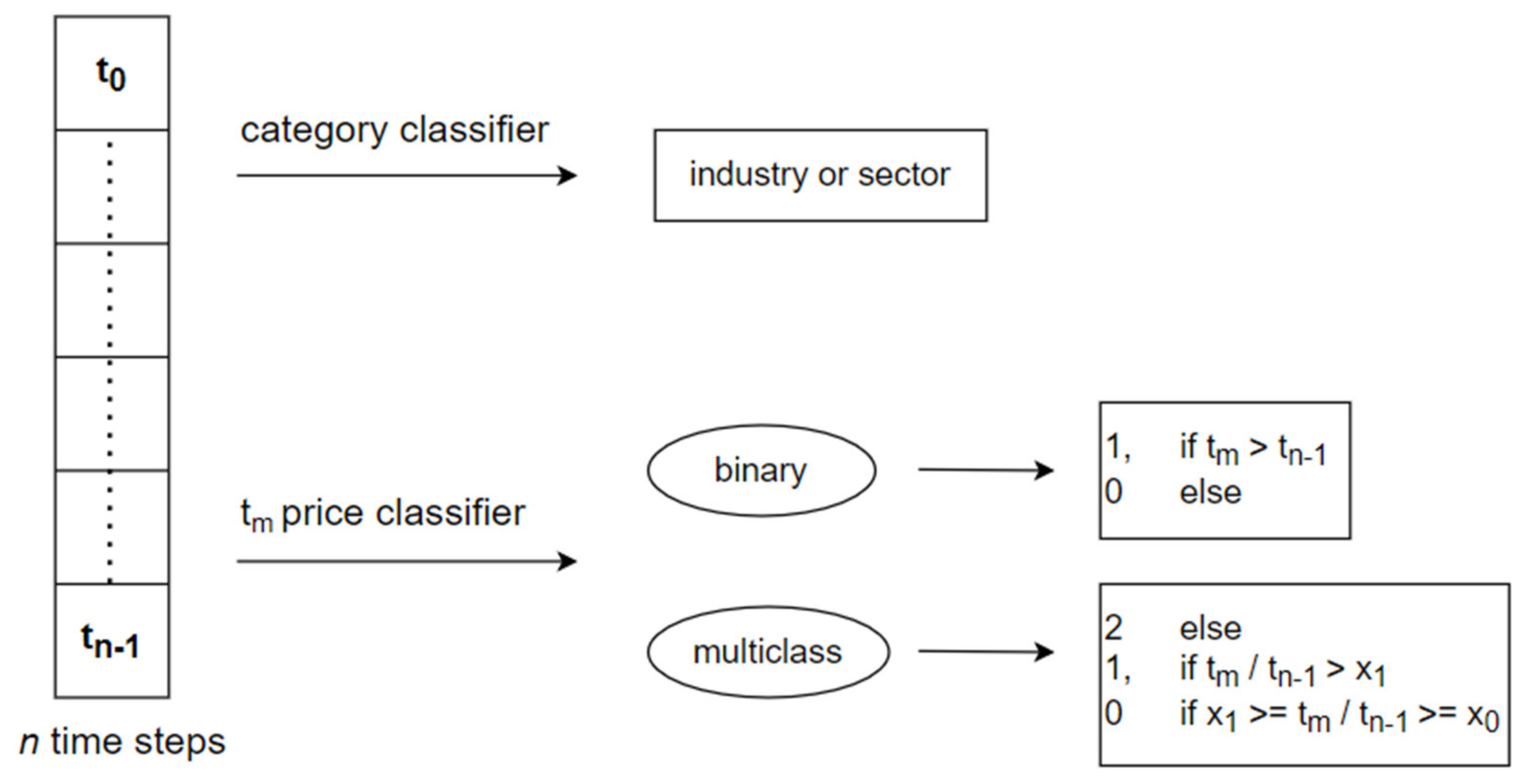
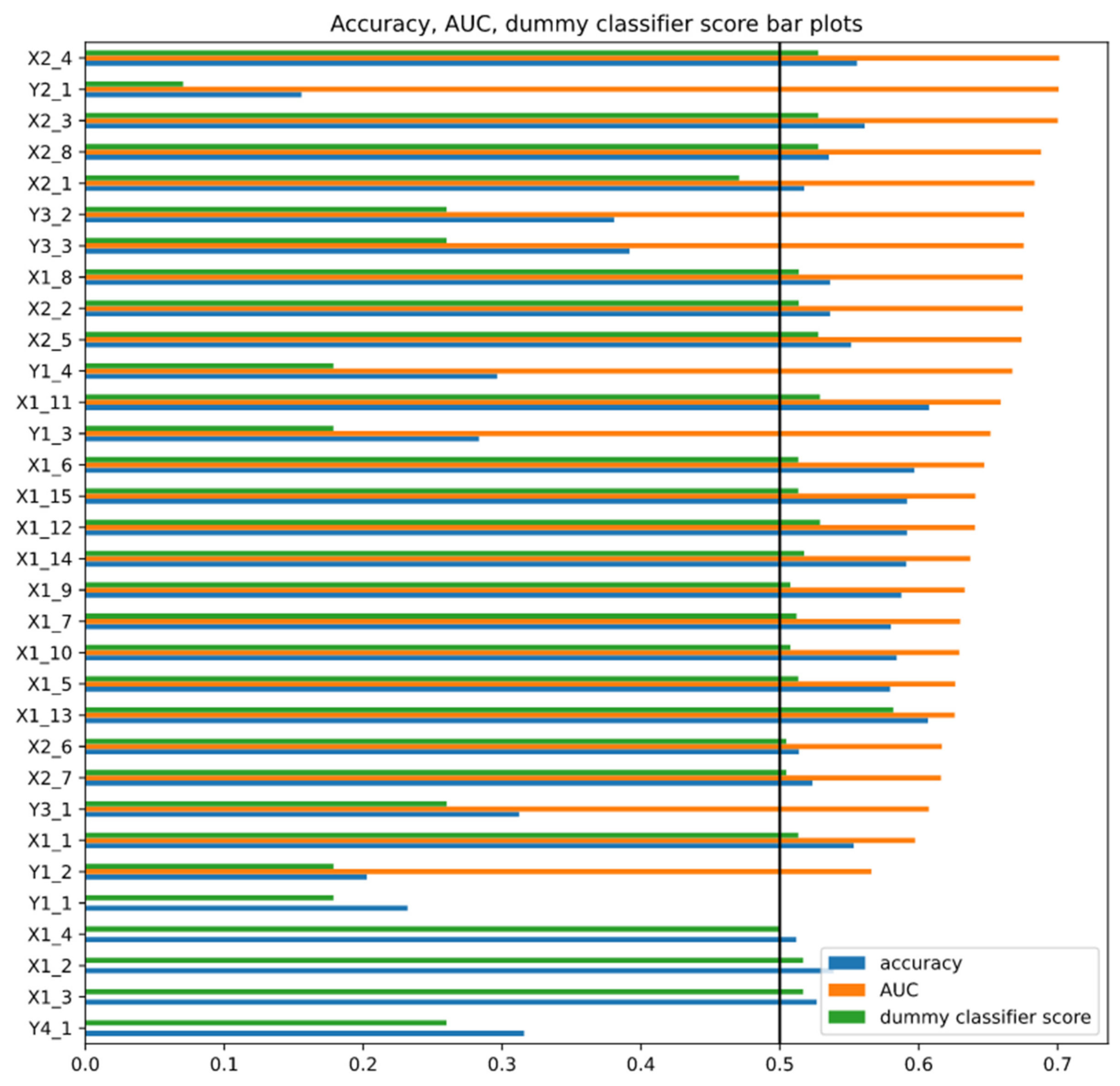
4.2. Convolutional Neural Network Training
- 15 binary classifiers;
- Eight multiclass classifiers;
- Four sector classifiers;
- Three sector top five classifiers;
- One industry classifier; and
- One industry top 10 classifier.
4.3. Cluster Analysis
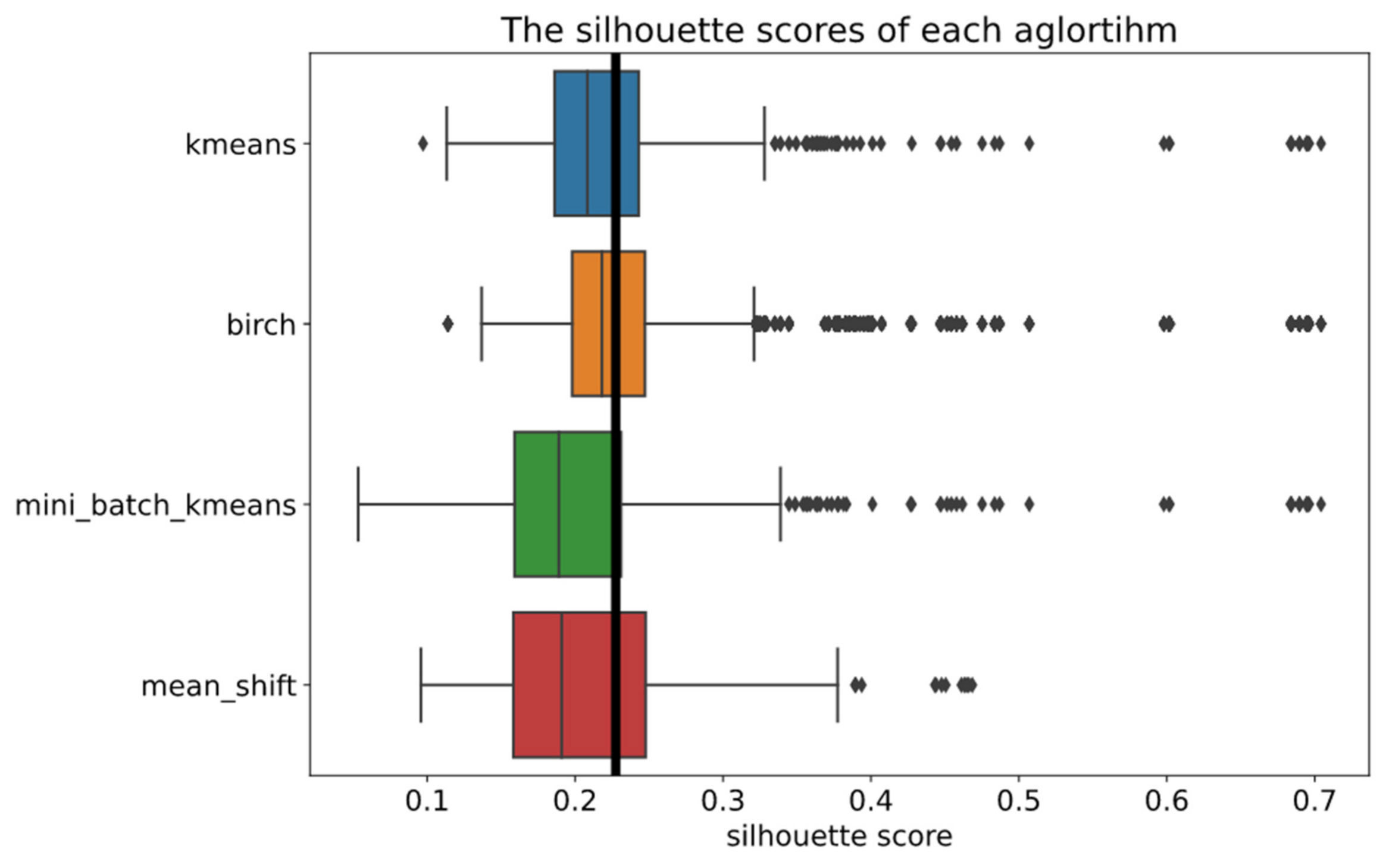
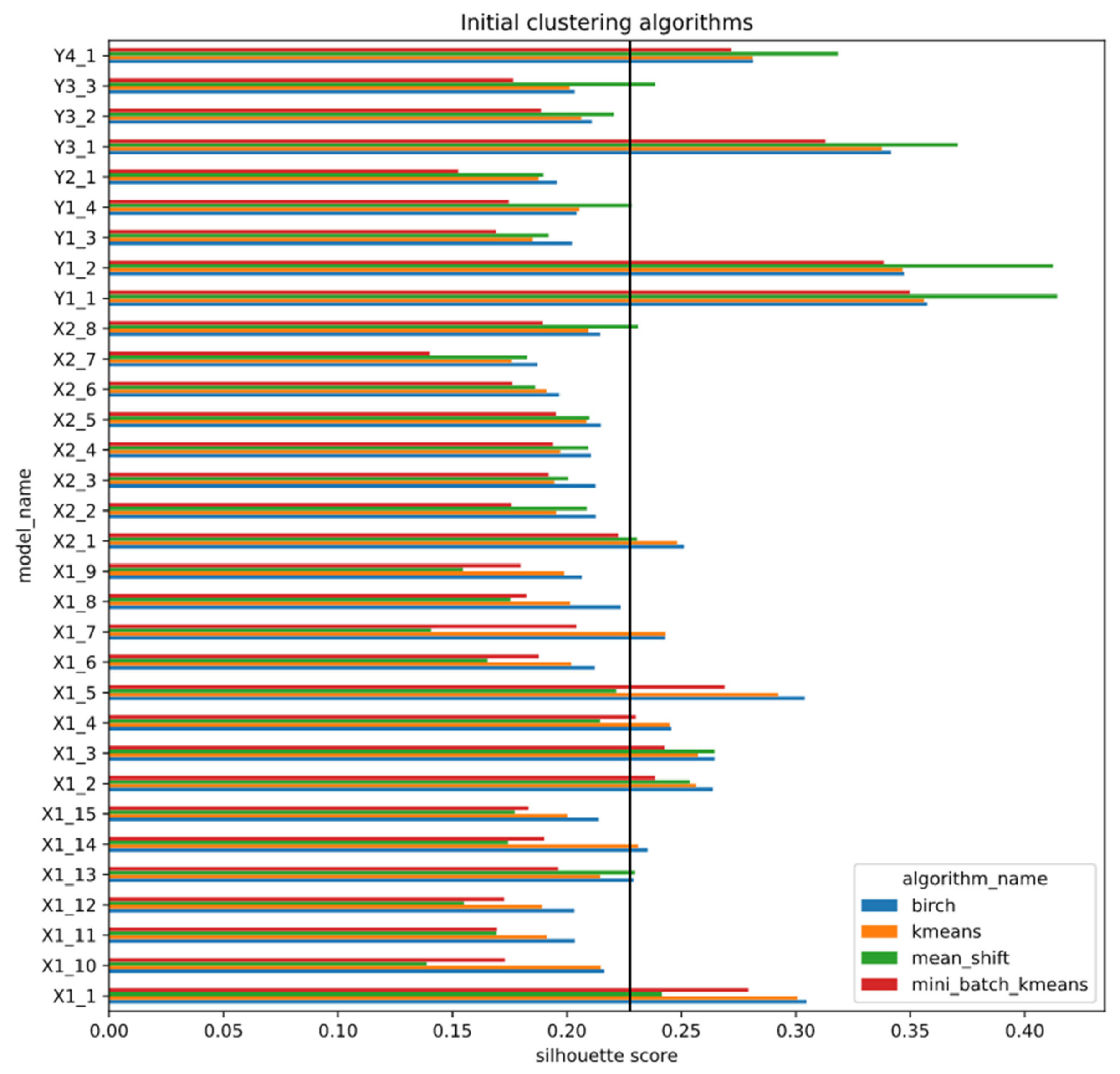
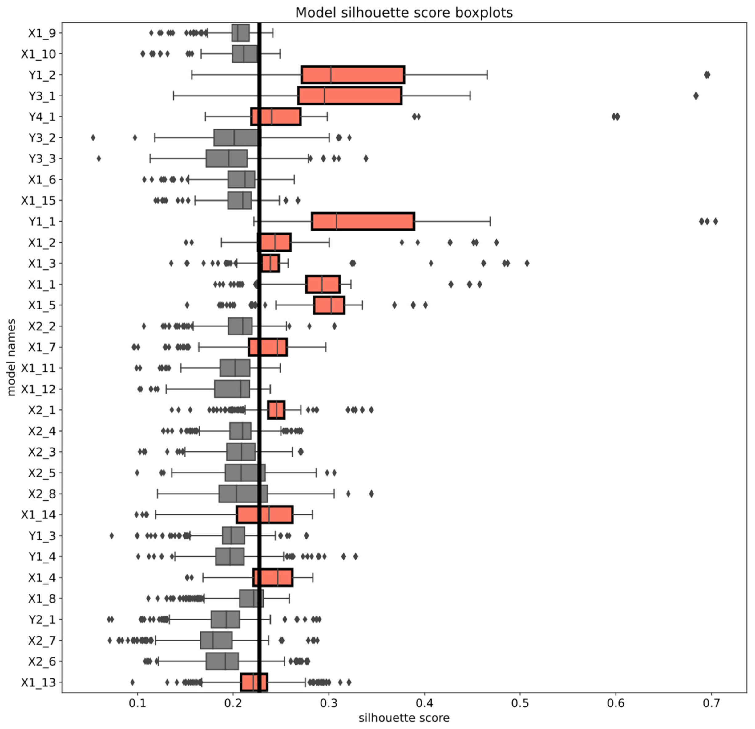
4.3.1. Initial Clustering Methods
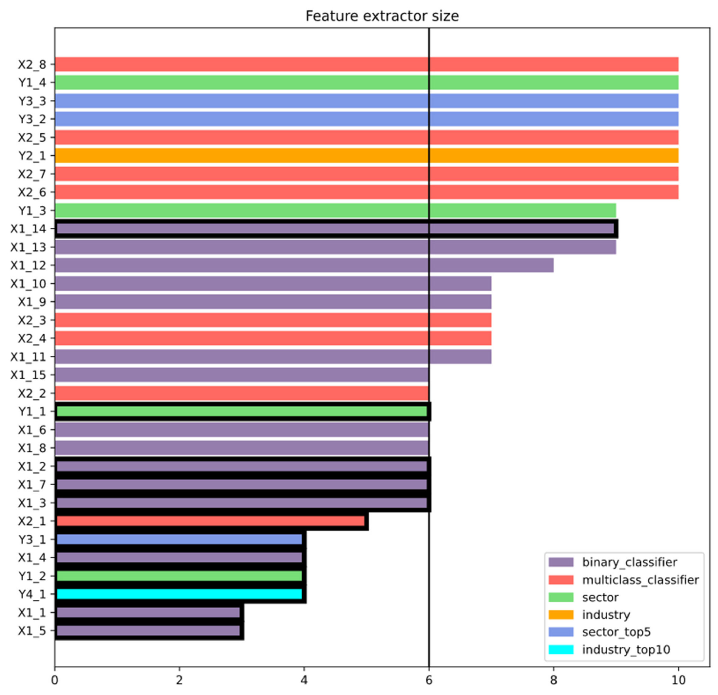
- Seven out of 15 binary models;
- One out of eight multiclass classifiers;
- Two out of four sector classifiers;
- One out of three sector top 5 classifiers;
- One out of one industry top 10 classifier.
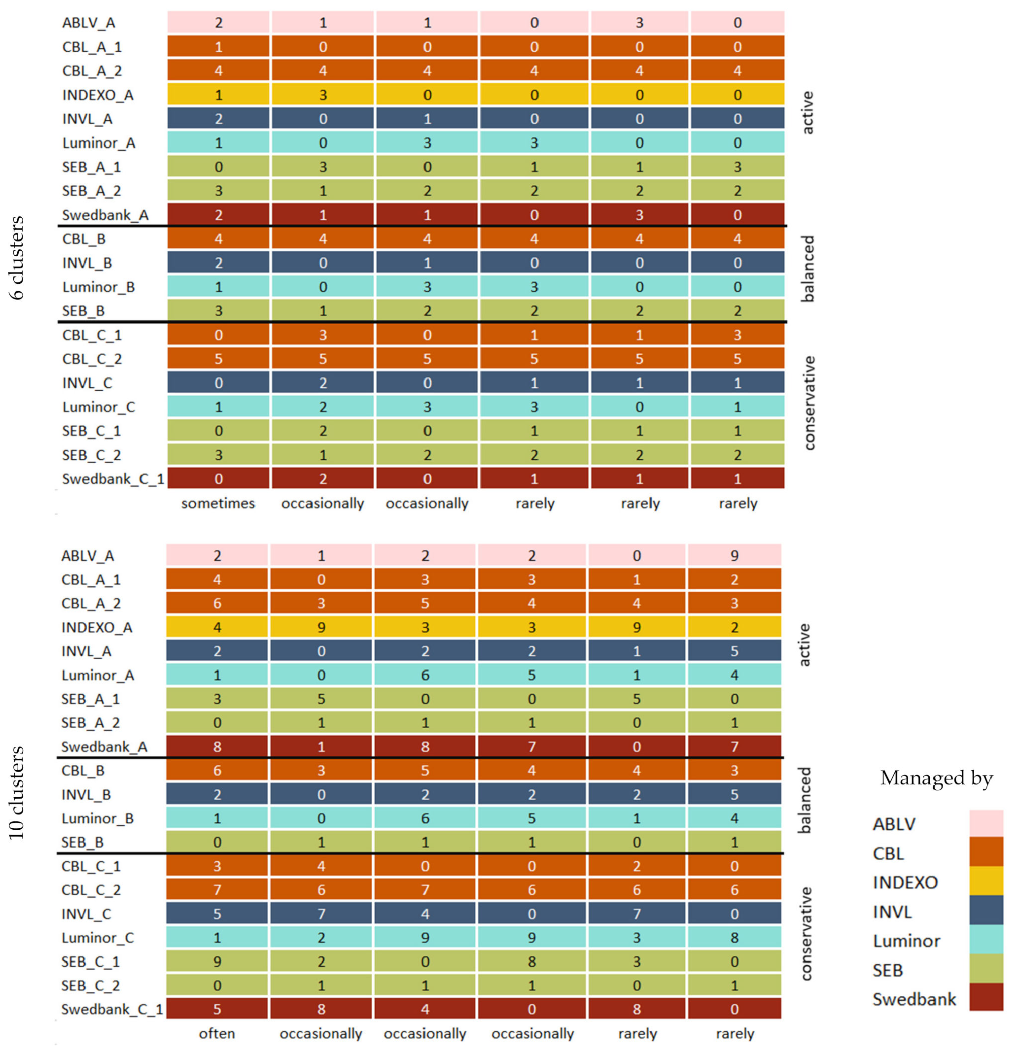
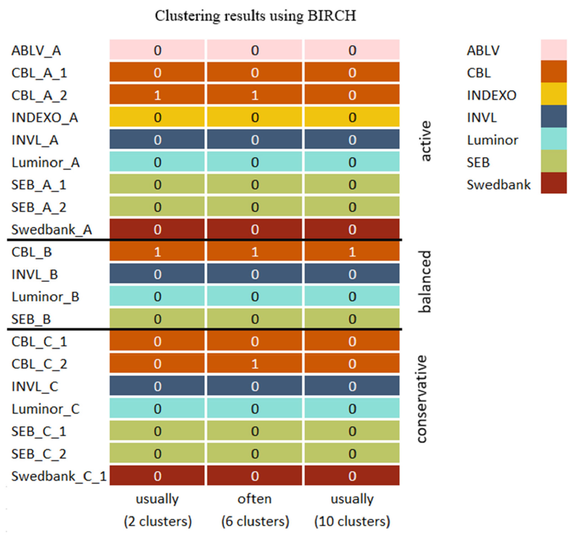
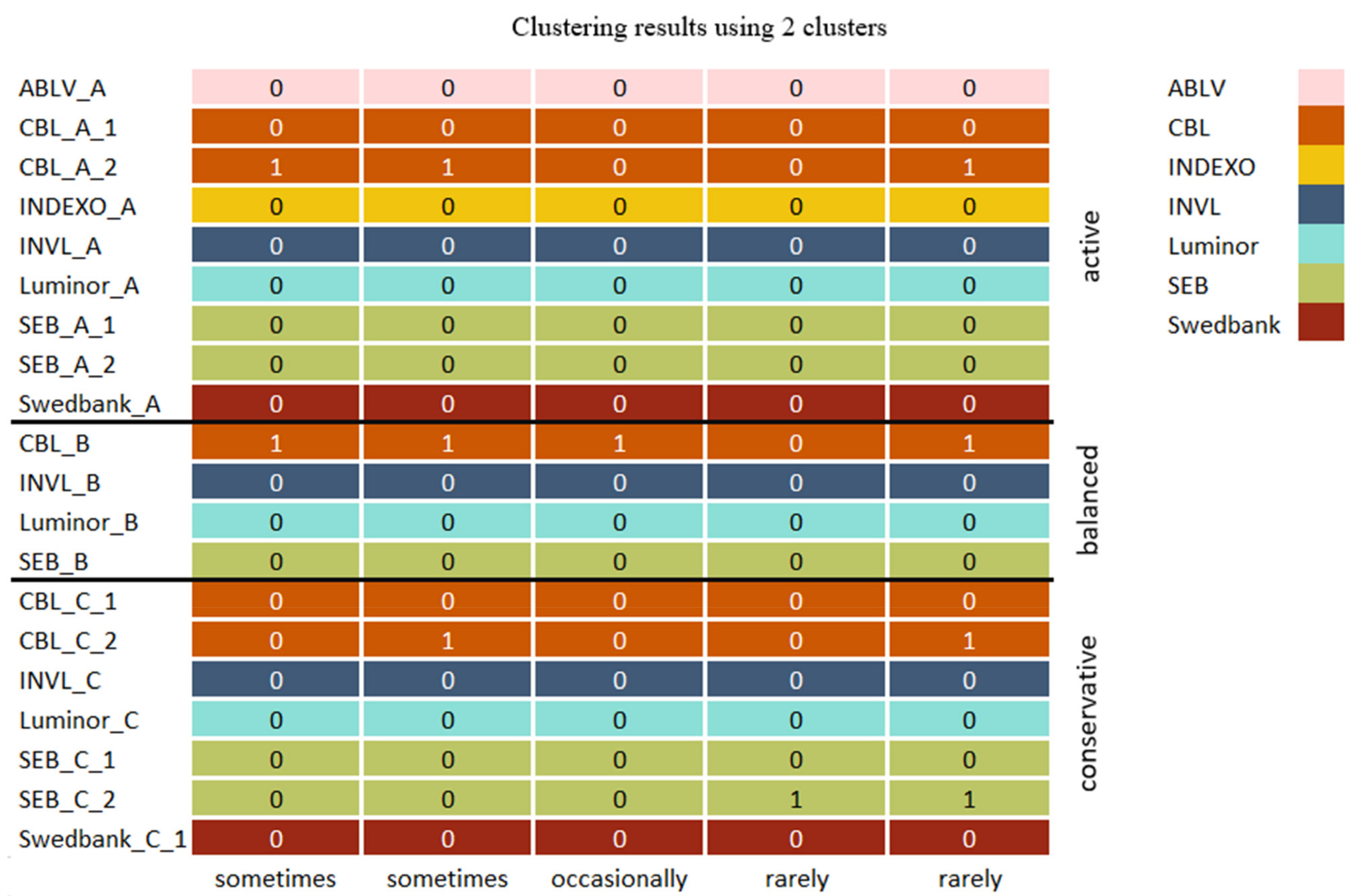
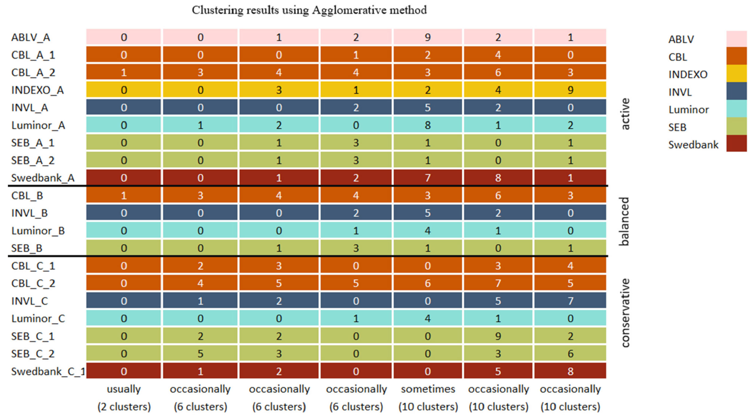
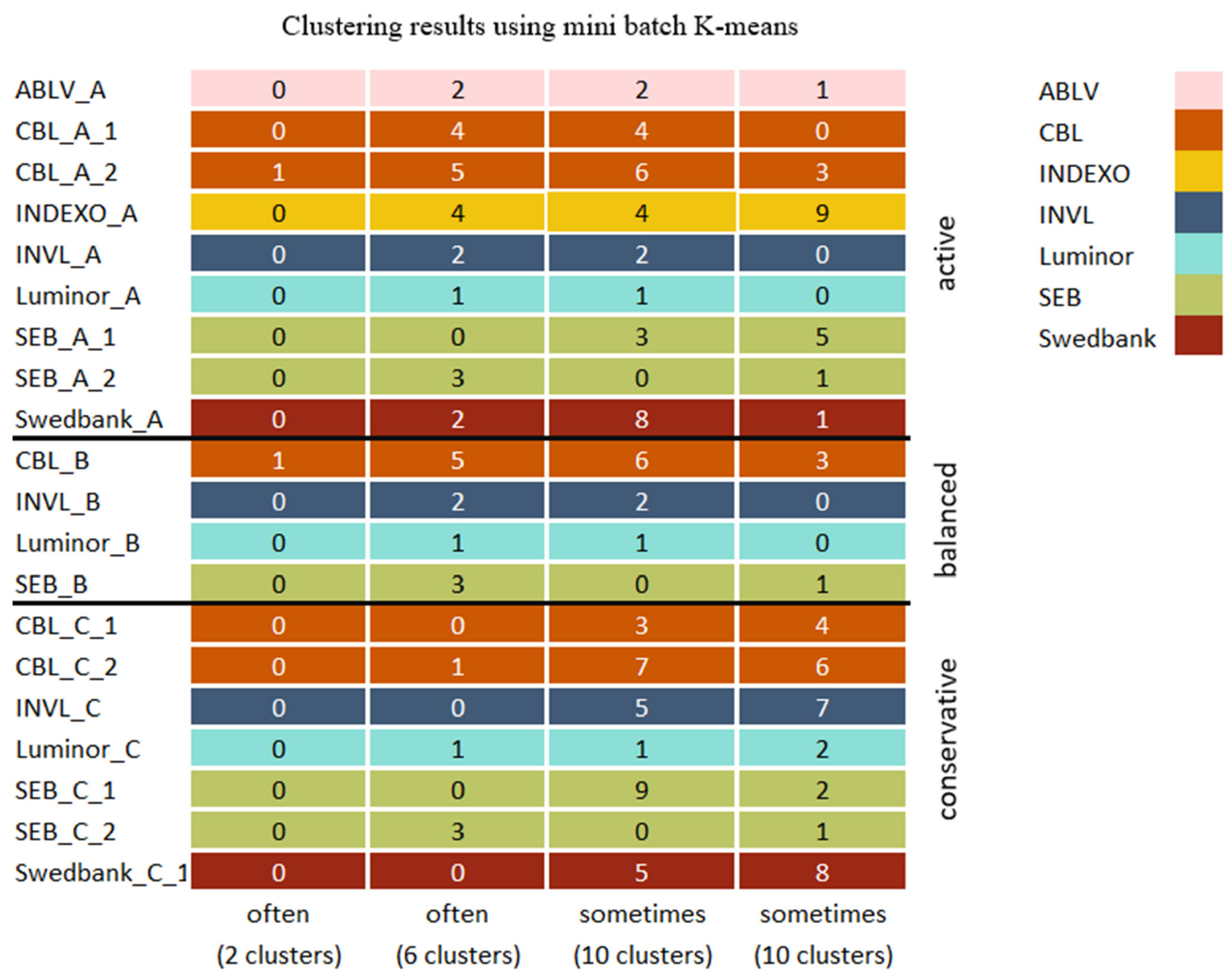
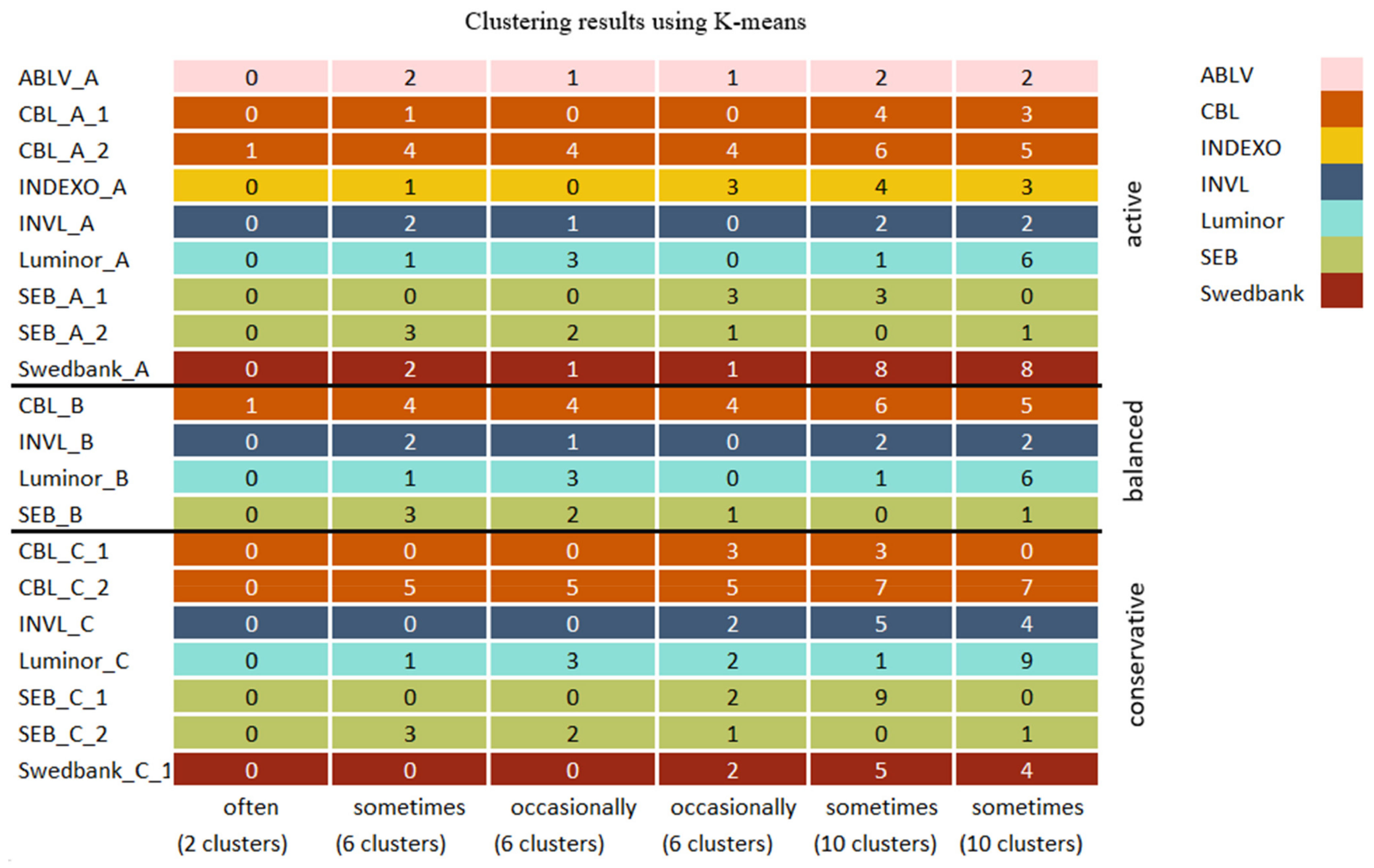
4.3.2. Clustering Methods of Pension Funds
4.4. The Interpretation of Results and Discussions
5. Conclusions
- Conservative, balanced, and active Luminor pension fund grouping.
- Grouping of two active and one conservative SEB pension funds.
- A consistent subgroup of CBL active and balanced pension funds.
Author Contributions
Funding
Data Availability Statement
Acknowledgments
Conflicts of Interest
Abbreviations and Terms
| EU | European union; |
| DC | defined contribution; |
| DB | defined benefit; |
| AI | artificial intelligence; |
| ANN | artificial neural networks. |
| CNN | convolutional neural network. |
| OECD | organization for economic co-operation and development; |
| BIRCH | balanced iterative reducing and clustering using hierarchies; |
| DBSCAN | density-based spatial clustering of applications with noise; |
| OPTICS | ordering points to identify the clustering structure. |
Appendix A. Trained Model Architectures, Clustering Algorithms, and Parameters

| Model Name and Classifier Type | Feature Extractor | Neural Network and Neurons |
|---|---|---|
| X1_6 (binary price classifier) | 16 kernels with size 2 | Dropout 896 |
| 32 kernels with size 3 | Dense 64 | |
| Max pooling | Dense 1 | |
| 64 kernels with size 5 | ||
| 128 kernels with size 5 | ||
| Max pooling | ||
| X1_15 (binary price classifier) | 16 kernels with size 2 | Dropout 896 |
| 32 kernels with size 3 | Dense 64 | |
| Max pooling | Dense 1 | |
| 64 kernels with size 5 | ||
| 128 kernels with size 5 | ||
| Max pooling | ||
| X2_1 (multiclass price classifier) | 32 kernels with size 2 | Dropout 1736 |
| 64 kernels with size 3 | Dense 256 | |
| Max pooling | Dropout | |
| 124 kernels with size 5 | Dense 64 | |
| Max pooling | Dense 3 | |
| X2_4 (multiclass price classifier) X2_3 (multiclass price classifier) | 32 kernels with size 2 | Dropout 3072 |
| 64 kernels with size 3 | Dense 64 | |
| 64 kernels with size 3 | Dense 3 | |
| Max pooling | ||
| 128 kernels with size 5 | ||
| 256 kernels with size 3 | ||
| Max pooling | ||
| Y1_1 (sector classifier) | 16 kernels with size 2 | Flatten 320 |
| Max pooling | Dense 64 | |
| 32 kernels with size 2 | Dense 12 | |
| Max pooling | ||
| 64 kernels with size 2 | ||
| Max pooling | ||
| Y1_2 (sector classifier) | 32 kernels with size 2 | Dropout 256 |
| Max pooling stride 3 | Dense 64 | |
| 64 kernels with size 2 | Dense 12 | |
| Max pooling stride 3 | ||
| X1_4 (binary price classifier) | 32 kernels with size 2 | Dropout 512 |
| Max pooling stride 2 | Dense 32 | |
| 32 kernels with size 2 | Dense 1 | |
| Max pooling stride 2 | ||
| Y2_1 (industry classifier) | 32 kernels with size 2 | Dropout 2304 |
| 64 kernels with size 3 | Dense 64 | |
| 64 kernels with size 2 | Dense 128 | |
| Max pooling | ||
| 128 kernels with size 2 | ||
| 256 kernels with size 3 | ||
| Max pooling | ||
| 256 kernels with size 3 | ||
| 256 kernels with size 3 | ||
| Max pooling | ||
| X2_2 (multiclass price classifier) | 64 kernels with size 2 | Dropout 2304 |
| 128 kernels with size 3 | Dense 256 | |
| Max pooling | Dense 64 | |
| 128 kernels with size 5 | Dense 3 | |
| 256 kernels with size 2 | ||
| Max pooling | ||
| X2_7 (multiclass price classifier) X2_6 (multiclass price classifier) | 32 kernels with size 2 | Dropout 2560 |
| 64 kernels with size 2 | Dense 256 | |
| 64 kernels with size 3 | Dense 64 | |
| Max pooling | Dense 3 (used range 5) | |
| 128 kernels with size 2 | ||
| 256 kernels with size 3 | ||
| Max pooling | ||
| 256 kernels with size 2 | ||
| 256 kernels with size 2 | ||
| Max pooling | ||
| X1_14 (binary price classifier) X1_13 (binary price classifier) | 32 kernels with size 2 | Dropout 1265, 2530 |
| 64 kernels with size 3 | Dense 256 | |
| 64 kernels with size 5 | Dense 64 | |
| Max pooling | Dense 1 | |
| 128 kernels with size 2 | ||
| 256 kernels with size 3 | ||
| Max pooling | ||
| 253 kernels with size 3 | ||
| Max pooling | ||
| X1_8 (binary price classifier) X1_7 (binary price classifier) | 64 kernels with size 2 | Dropout 4096, 2304 |
| 128 kernels with size 3 | Dense 256 | |
| Max pooling | Dense 64 | |
| 128 kernels with size 5 | Dense 1 | |
| 256 kernels with size 2 | ||
| Max pooling | ||
| X1_9 (binary price classifier) X1_10 (binary price classifier) X1_11 (binary price classifier) | 32 kernels with size 2 | Dropout 1280, 2560 |
| 64 kernels with size 3 | Dense 64 | |
| 64 kernels with size 3 | Dense 1 | |
| Max pooling | ||
| 128 kernels with size 5 | ||
| 256 kernels with size 3 | ||
| Max pooling | ||
| X1_12 (binary price classifier) | 64 kernels with size 2 | Dropout 1024 |
| 64 kernels with size 3 | Dense 256 | |
| Max pooling | Dense 64 | |
| 128 kernels with size 2 | Dense 1 | |
| Max pooling | ||
| 128 kernels with size 6 | ||
| 256 kernels with size 3 | ||
| Max pooling | ||
| Y3_1 (sector classifier taking top 5 most frequent sectors) | 32 kernels with size 2 | Dropout 288 |
| Max pooling | Dense 32 | |
| 32 kernels with size 2 | Dense 5 | |
| Max pooling | ||
| Y3_2 (sector classifier taking top 5 most frequent sectors) Y3_3 (sector classifier taking top 5 most frequent sectors) | 32 kernels with size 2 | Dropout 512 |
| 64 kernels with size 3 | Dense 64 | |
| 64 kernels with size 2 | Dense 5 | |
| Max pooling | ||
| 128 kernels with size 2 | ||
| 256 kernels with size 3 | ||
| Max pooling | ||
| 256 kernels with size 3 | ||
| 256 kernels with size 3 | ||
| Max pooling | ||
| Y1_3 (sector classifier) | 32 kernels with size 2 | Dropout 1265 |
| 64 kernels with size 3 | Dense 64 | |
| 64 kernels with size 2 | Dense 12 | |
| Max pooling | ||
| 128 kernels with size 2 | ||
| 256 kernels with size 3 | ||
| Max pooling | ||
| 253 kernels with size 2 | ||
| Y1_4 (sector classifier) X1_2 (binary price classifier) | 32 kernels with size 2 | Dropout 1024, 1408 |
| 64 kernels with size 3 | Dense 64 | |
| 64 kernels with size 2 | Dense 12, 1 | |
| Max pooling | ||
| 128 kernels with size 2 | ||
| 256 kernels with size 3 | ||
| Max pooling | ||
| 256 kernels with size 3 | ||
| 256 kernels with size 3 | ||
| X1_3 (binary price classifier) | 16 kernels with size 2 | Dropout 1408 |
| 32 kernels with size 2 | Dense 64 | |
| Max pooling | Dense 1 | |
| 64 kernels with size 2 | ||
| 128 kernels with size 2 | ||
| Max pooling | ||
| X1_1 (binary price classifier) X1_5 (binary price classifier) | 64 kernels with size 2 | Dropout 256 |
| 128 kernels with size 3 | Dense 64 | |
| Max pooling | Dense 1 | |
| Y4_1 (industry classifier taking top 100 most frequent industries) | 32 kernels with size 2 | Dropout 288 |
| Max pooling | Dense 32 | |
| 32 kernels with size 2 | Dense 10 | |
| Max pooling | ||
| X2_5 (multiclass price classifier) | 32 kernels with size 2 | Dropout 768 |
| 64 kernels with size 3 | Dense 64 | |
| 64 kernels with size 2 | Dense 3 | |
| Max pooling | ||
| 128 kernels with size 5 | ||
| 128 kernels with size 3 | ||
| Max pooling | ||
| 256 kernels with size 3 | ||
| 256 kernels with size 5 | ||
| Max pooling | ||
| X2_8 (multiclass price classifier) | 32 kernels with size 2 | Dropout 256 |
| 64 kernels with size 3 | Dense 64 | |
| 64 kernels with size 3 | Dense 3 | |
| Max pooling | ||
| 128 kernels with size 4 | ||
| 128 kernels with size 5 | ||
| Max pooling | ||
| 256 kernels with size 3 | ||
| 256 kernels with size 3 | ||
| Max pooling |
| Model Name | Input Size | Predict Price Timestep | Overlap | Epochs | Accuracy | AUC | Dummy Score |
|---|---|---|---|---|---|---|---|
| X1_15 | 50 | 5 | 5 | 300 | 0.5916 | 0.6408 | 0.5133 |
| X1_6 | 50 | 5 | 5 | 400 | 0.5969 | 0.6472 | 0.5133 |
| X1_5 | 50 | 5 | 0 | 400 | 0.5794 | 0.6263 | 0.5133 |
| X2_1 | 60 | 5 | 0 | 300 | 0.5176 | 0.6834 | 0.4707 |
| X2_5 | 60 | 5 | 0 | 200 | 0.5514 | 0.6741 | 0.5277 |
| X2_8 | 60 | 5 | 0 | 200 | 0.5353 | 0.6881 | 0.5277 |
| X2_3 | 60 | 5 | 5 | 200 | 0.5611 | 0.7002 | 0.5277 |
| X2_4 | 60 | 5 | 10 | 200 | 0.5556 | 0.7012 | 0.5277 |
| X1_9 | 30 | 5 | 5 | 100 | 0.5875 | 0.6331 | 0.5076 |
| X1_10 | 30 | 5 | 5 | 100 | 0.5841 | 0.6292 | 0.5076 |
| X1_11 | 50 | 5 | 5 | 200 | 0.6074 | 0.6590 | 0.5289 |
| X1_14 | 60 | 10 | 10 | 100 | 0.5910 | 0.6371 | 0.5175 |
| X1_13 | 100 | 80 | 30 | 100 | 0.6067 | 0.6259 | 0.5817 |
| X2_7 | 100 | 80 | 30 | 200 | 0.5235 | 0.6160 | 0.5047 |
| X2_6 | 100 | 80 | 30 | 100 | 0.5137 | 0.6167 | 0.5047 |
| Y1_3 | 60 | - | 0 | 200 | 0.2834 | 0.6516 | 0.1786 |
| Y1_4 | 60 | - | 0 | 200 | 0.2965 | 0.6674 | 0.1786 |
| Y3_2 | 40 | - | 0 | 200 | 0.3807 | 0.6759 | 0.2601 |
| Y3_3 | 40 | - | 0 | 205 | 0.3918 | 0.6756 | 0.2601 |
| Y2_1 | 100 | - | 0 | 400 | 0.1556 | 0.7007 | 0.0704 |
| X1_12 | 50 | 5 | 5 | 200 | 0.5915 | 0.6405 | 0.5289 |
| X2_2 | 50 | 15 | 20 | 200 | 0.5361 | 0.6749 | 0.5136 |
| X1_8 | 80 | 15 | 20 | 200 | 0.5800 | 0.6298 | 0.512 |
| Y1_1 | 50 | - | 0 | 200 | 0.2320 | - | 0.1786 |
| X1_4 | 70 | 7 | 0 | 200 | 0.5118 | - | 0.5 |
| Y1_2 | 40 | - | 0 | 150 | 0.2026 | 0.5659 | 0.1786 |
| X1_7 | 50 | 15 | 20 | 200 | 0.5800 | 0.6298 | 0.5120 |
| Y3_1 | 40 | - | 0 | 180 | 0.3123 | 0.6072 | 0.2601 |
| X1_2 | 50 | 5 | 0 | 200 | 0.5388 | - | 0.5168 |
| X1_3 | 50 | 10 | 0 | 200 | 0.5265 | - | 0.5168 |
| X1_1 | 50 | 5 | 0 | 400 | 0.5532 | 0.5974 | 0.5133 |
| Y4_1 | 40 | - | 0 | 200 | 0.3159 | - | 0.26 |
| Algorithm Name | Parameter Name | Parameter Value | |
|---|---|---|---|
| K-means, mini batch K-means | n_clusters | 2 to 10 | |
| Birch | n_clusters | 2 to 10 | |
| threshold | 0.1 to 1 with 0.1 step | ||
| Mean shift | bin_seeding | true, false | |
| cluster_all | true, false | ||
| Affinity propagation | damping | 0.5 to 1 with 0.05 step | |
| DBSCAN | eps | 0.3, 0.5 or 0.8 | |
| Optics | leaf_size | 30 | |
| DBSCAN, Optics | min_samples | 3, 5 or 10 | |
| algorithm, metric | kd_tree | Euclidean, l2, Minkowski, Manhattan, Chebyshev | |
| ball_tree | Euclidean, L2, Minkowski, Manhattan, L1, Chebyshev, Wminkowski, Canberra, Bray–Curtis | ||
| brute | Euclidean, L2, Minkowski, Manhattan, Chebyshev, Wminkowski, Canberra, Braycurtis, Correlation, Cosine, Squeclidean | ||
| Agglomerative | n_clusters | 2 to 10 | |
| linkage | Ward, Average, Complete, or single | ||
| affinity | Euclidean, L1, L2, Manhattan, Cosine | ||
Appendix B. Clustering Results


| Cluster 0 | Cluster 1 | Cluster 2 | Cluster 3 | Cluster 4 | Cluster 5 |
|---|---|---|---|---|---|
| CBL_C_1 INVL_C SEB_C_1 SEB_C_2 Swedbank_C_1 | CBL_A_1 INDEXO_A Luminor_A Luminor_B Luminor_C | ABLV_A INVL_A INVL_B Swedbank_A | SEB_A_1 SEB_A_2 SEB_B | CBL_A_2 CBL_B | CBL_C_2 |
Appendix C. Best Parameters and Models for Each Clustering Algorithm
| Algorithm Name | Clusters | Total Combinations | Mean Silhouette Score | Top Taken | Mean Silhouette Score Top | Best Model | Algorithm Parameters |
|---|---|---|---|---|---|---|---|
| K-means | 2 | 152 | 0.2638 | 10 | 0.6916 | Y1_1, Y1_2, Y3_1 | - |
| K-means | 6 | 152 | 0.2184 | 10 | 0.31 | Y1_1 | - |
| K-means | 10 | 152 | 0.2064 | 10 | 0.2931 | X1_5, X1_1, Y1_1 | - |
| BIRCH | 2 | 1368 | 0.2746 | 10 | 0.7035 | Y1_1 | - |
| BIRCH | 6 | 1368 | 0.228 | 10 | 0.3266 | X1_5 | - |
| BIRCH | 10 | 1368 | 0.2165 | 10 | 0.314 | X1_5 | - |
| Mini batch K-means | 2 | 152 | 0.2556 | 10 | 0.6916 | Y1_1, Y1_2, Y3_1 | - |
| Mini batch K-means | 6 | 152 | 0.2017 | 10 | 0.303 | Y1_1, Y1_2, Y3_1 | - |
| Mini batch K-means | 10 | 152 | 0.1777 | 10 | 0.2788 | X1_5 | - |
| Mean shift | 2 | 117 | 0.1856 | 10 | 0.2859 | Y2_1, X2_7 | - |
| Agglomerative clustering | 2 | 400 | 0.421 | 10 | 0.8666 | Y1_1, Y1_2, Y3_1 | Affinity: cosine |
| Agglomerative clustering | 6 | 400 | 0.2216 | 10 | 0.4354 | - | Linkage: average or complete; Affinity: cosine |
| Agglomerative clustering | 10 | 400 | 0.2125 | 10 | 0.4293 | - | Linkage: average or complete; Affinity: cosine |
| OPTICS | 2 | 382 | 0.0813 | 10 | 0.3825 | X1_3 | - |
| OPTICS | 10 | 1 | 0.1928 | 1 | 0.1928 | X1_14 | Algorithm: ball_tree; Metric: Bray–Curtis |
| DBSCAN | 2 | 321 | 0.4583 | 10 | 0.8349 | Y1_1, Y1_2, Y3_1 | Algorithm: brute; Metric: correlation, Bray-Curtis |
| Affinity propagation | 6 | 99 | 0.2052 | 10 | 0.286 | Y1_1, X1_5 | Damping: 0.5, 0.55, 0.6 |
References
- Ganguli, S.; Dunnmon, J. Machine Learning for Better Models for Predicting Bond Prices. 2017. Available online: https://arxiv.org/abs/1705.01142 (accessed on 11 May 2021).
- OECD. Pension Market in Focus. 2019. Available online: https://www.oecd.org/daf/fin/private-pensions/Pension-Markets-in-Focus-2019.pdf (accessed on 11 May 2021).
- Kotecha, M.; Arthur, S.; Coutinho, S. Understanding the Relationship Between Pensioner Poverty and Material Deprivation, London. 2013; ISBN 9781909532144. Available online:https://assets.publishing.service.gov.uk/government/uploads/system/uploads/attachment_data/file/197675/rrep827.pdf (accessed on 11 May 2021).
- Lannoo, K.; Barslund, M.; Chmelar, A.; Werder, M.; Pension Schemes. Brussels, 2014: European Parliament’s Committee on Employment and Social Affairs. Available online: https://www.europarl.europa.eu/RegData/etudes/STUD/2014/536281/IPOL_STU(2014)536281_EN.pdf (accessed on 11 May 2021).
- Keohane, N.; Rowell, S.; Good Pensions. Introducing Social Pension Funds to the UK, London: Social Market Foundation. 2015. Available online: http://www.smf.co.uk/wp-content/uploads/2015/09/Social-Market-FoundationSMF-BSC-030915-Good-Pensions-Introducing-social-pension-funds-to-the-UK-FINAL.pdf (accessed on 11 May 2021).
- Pensions Europe. Pension Fund Statistics and Trends 2018. Available online: https://www.pensionseurope.eu (accessed on 11 May 2021).
- Bruder, B.; Culerier, L.; Roncalli, T. How to design target-date funds? SSRN Electron. J. 2013. [Google Scholar] [CrossRef]
- Donaldson, S.J.; Kinniry, F.M.; Mačiulis, V.; Patterson, A.J.; Dijoseph, M. Vanguard’s approach to target-date funds [interactive]. Available online: https://www.vanguard.com/ (accessed on 11 May 2021).
- Laursen, C.; Gkatzimas, I.; Jovanovic, B. TARGET DATE FUNDS Economic, Regulatory, and Legal Trends. 2017. Available online: https://brattlefiles.blob.core.windows.net/files/7164_target_date_funds_economic__regulatory__and_legal_trends.pdf (accessed on 11 May 2021).
- Tonks, I. Pension Fund Management and Investment Performance; Gordon, L.C., Munnell, A.H., Orszag, J.M., Eds.; The Oxford Handbook of Pensions and Retirement Income: Oxford, UK, 2006. [Google Scholar]
- Keeley, B.; Love, P. OECD Insights from Crisis to Recovery the Causes, Course and Consequences of the Great Recession: The Causes, Course and Consequences of the Great Recession; OECD Publishing: Paris, France, 2010. [Google Scholar] [CrossRef]
- Manapensija: Current Statistics. Available online: https://www.manapensija.lv/en/2nd-pension-pillar/statistics/ (accessed on 30 April 2021).
- Kabašinskas, A.; Maggioni, F.; Šutienė, K.; Valakevičius, E. A Multistage Risk-Averse Stochastic Programming Model for Personal Savings Accrual: The Evidence from Lithuania—Annals of Operations Research; Springer: New York, NY, USA, 2018; pp. 1–28. ISSN 0254-5330. [Google Scholar] [CrossRef]
- Financial and Capital Market Commission. Available online: https://www.fktk.lv/ (accessed on 10 August 2021).
- Jefremova, J.; Mietule, I. Investment trends of Latvian pension funds after the 2008 financial crisis. In Proceedings of the 5th International Conference on Accounting, Auditing and Taxation, Tallinn, Estonia, 8–9 December 2016. [Google Scholar] [CrossRef]
- Rajevska, O.; Rajevska, F. Effectiveness of the Latvian pension system in addressing the problem of poverty among the elderly. In Proceedings of the Pensions Conference 2018, Lodz, Poland, 19–20 April 2018. [Google Scholar]
- Serge-Lopez, W.-T.; Wamba, S.F.; Kamdjoug, J.R.K.; Wanko, C.E.T.W. Influence of Artificial Intelligence (AI) on firm performance: The business value of AI-based transformation projects. Bus. Process. Manag. J. 2020, 26, 1893–1924. Available online: https://www.emerald.com/insight/content/doi/10.1108/BPMJ-10-2019-0411/full/html#loginreload (accessed on 11 May 2021).
- Chen, M.Y.; Chiang, H.S.; Lughofer, E. Deep learning: Emerging trends, applications and research challenges. Soft Comput. 2020, 24, 7835–7838. [Google Scholar] [CrossRef]
- Zhao, B.; Lu, H.; Chen, S.; Liu, J.; Wu, D. Convolutional neural networks for time series classification. J. Syst. Eng. Electron. 2017, 28, 162–169. [Google Scholar] [CrossRef]
- Umuhoza, E.; Ntirushwamaboko, D.; Awuah, J.; Birir, B. Using unsupervised machine learning techniques for behavioral-based credit card users segmentation in Africa. S. Afr. Inst. Electr. Eng. 2020, 111, 95–101. Available online: http://www.scielo.org.za/pdf/arj/v111n3/02.pdf (accessed on 11 May 2021). [CrossRef]
- Xu, D.; Tian, Y. A comprehensive survey of clustering algorithms. Ann. Data Sci. 2015, 2, 165–193. [Google Scholar] [CrossRef]
- Javedac, A.; Leeac, B.S.; Rizzobc, D.M. A benchmark study on time series clustering. Mach. Learn. Appl. 2020, 1, 1–13. [Google Scholar]
- Lei, Q.; Yi, J.; Vaculin, R.; Wu, L.; Dhillon, I.S. Similarity preserving representation learning for time series clustering. In Proceedings of the Twenty Eighth International Joint Conference on Artificial Intelligence, Macao, China, 10–16 August 2019; {IJCAI-19} 2019. Available online: https://www.ijcai.org/proceedings/2019/394 (accessed on 11 May 2021).
- Guerin, J.; Gibaru, O.; Thiery, S.; Nyiri, E. CNN features are also great at unsupervised classification [interactive]. arXiv 2017, arXiv:1707.01700. [Google Scholar]
- Chen, W.; Langrene, N. Deep Neural Network for Optimal Retirement Consumption in Defined Contribution Pension System 2020. Available online: https://arxiv.org/pdf/2007.09911.pdf (accessed on 10 May 2021).
- Sasaki, T.; Koizumi, H.; Tajiri, T.; Kitano, H. A Study on the Use of Artificial Intelligence within Government Pension Investment Fund’s Investment Management Practices (Summary Report), Tokyo, 2017: Government Pension Investment Fund. Available online: https://www.gpif.go.jp/en/investment/research_2017_1_en.pdf (accessed on 11 May 2021).
- Barna, F.; Seulean, V.; Mos, M.L. A cluster analysis of OECD pension funds. Timis. J. Econ. 2011, 4, 143–148. [Google Scholar]
- Kabašinskas, A.; Šutienė, K.; Kopa, M.; Valakevičius, E. The risk-return profile of Lithuanian private pension funds. Ecnonomic Res. 2017, 30, 1611–1630. [Google Scholar] [CrossRef]
- Kaggle: Daily Historical Stock Prices 1970–2018. Available online: https://www.kaggle.com/ehallmar/daily-historical-stock-prices-1970-2018 (accessed on 10 March 2021).
- Keras. Developer Guides. Available online: https://keras.io/guides/ (accessed on 11 May 2021).
- Wandb. Fundamentals of Neural Networks. 2019. Available online: https://wandb.ai/site/articles/fundamentals-of-neural-networks (accessed on 11 May 2021).
- Kingma, D.P.; Lei, B.; Adam, J. A Method for Stochastic Optimization. 2015. Available online: https://arxiv.org/abs/1412.6980 (accessed on 10 May 2021).
- Yoon, K. Convolutional Neural Networks for Sentence Classification. 2014. Available online: https://arxiv.org/pdf/1408.5882.pdf (accessed on 11 May 2021).
- Meysam, V.; Mohammad, G.; Masoumeh, R. Learning Algorithms for IoT Data Classification, Preprint 2020. Available online: https://www.researchgate.net/publication/338853237_Performance_Analysis_and_Comparison_of_Machine_and_Deep_Learning_Algorithms_for_IoT_Data_Classification (accessed on 11 May 2021).
- Sklearn. Clustering. Available online: https://scikit-learn.org/stable/modules/clustering.html (accessed on 11 May 2021).
- Mercioni, M.A.; Holban, S. A Survey of Distance Metrics in Clustering Data Mining Techniques. Conference: ICGSP ’19. 2019. Available online: https://dl.acm.org/doi/10.1145/3338472.3338490 (accessed on 11 May 2021).
- Alvarez-Gonzalez, P.; Forsberg, F. Unsupervised Machine Learning: An Investigation of Clustering Algorithms on a Small Dataset. Blekinge Institute of Technology, Karlskrona Sweden. 2018. Available online: https://www.diva-portal.org/smash/get/diva2:1213516/FULLTEXT01.pdf (accessed on 11 May 2021).
- Yosinski, J.; Clune, J.; Bengio, Y.; Lipson, H. How Transferable are Features in Deep Neural Networks? 2014. Available online: https://arxiv.org/abs/1411.1792 (accessed on 10 August 2021).


| Pension Fund Name | Encoded Name | Manager | Category |
|---|---|---|---|
| ABLV active investment plan | ABLV_A | ABLV | Active |
| CBL Aktivais ieguldijumu plans | CBL_A_1 | CBL | Active |
| Ieguldijumu plans “GAUJA” | CBL_A_2 | CBL | Active |
| Ieguldijumu plans “INDEXO Izaugsme 47–57” | INDEXO_A | INDEXO | Active |
| Ieguldijumu plans “INVL Ekstra 47+” | INVL_A | INVL | Active |
| Luminor Aktivais ieguldijumu plans | Luminor_A | Luminor | Active |
| SEB aktivais plans | SEB_A_1 | SEB | Active |
| SEB Eiropas plans | SEB_A_2 | SEB | Active |
| Swedbank pensiju ieguldijumu plans “Dinamika” | Swedbank_A | Swedbank | Active |
| Ieguldijumu plans “VENTA” | CBL_B | CBL | Balanced |
| Ieguldijumu plans “INVL Komforts 53+” | INVL_B | INVL | Balanced |
| Luminor Sabalansetais ieguldijumu plans | Luminor_B | Luminor | Balanced |
| SEB sabalansetais plans | SEB_B | SEB | Balanced |
| CBL Universalais ieguldijumu plans | CBL_C_1 | CBL | Conservative |
| Ieguldijumu plans “DAUGAVA” | CBL_C_2 | CBL | Conservative |
| Ieguldijumu plans “INVL Konservativais 58+” | INVL_C | INVL | Conservative |
| Luminor Konservativais ieguldijumu plans | Luminor_C | Luminor | Conservative |
| SEB konservativais plans | SEB_C_1 | SEB | Conservative |
| SEB Latvijas plans | SEB_C_2 | SEB | Conservative |
| Swedbank pensiju ieguldijumu plans “Stabilitate” | Swedbank_C_1 | Swedbank | Conservative |
| Encoding | Q1 | Mean | Q3 | Standard Deviation | Kurtosis | Skewness | Sharpe Ratio |
|---|---|---|---|---|---|---|---|
| ABLV_A | −0.00206 | 0.0002 | 0.00296 | 0.00562 | 16.424 | −1.865 | 0.03596 |
| CBL_A_1 | −0.00099 | 0.00016 | 0.00176 | 0.00323 | 14.066 | −1.675 | 0.04872 |
| CBL_C_1 | −0.00046 | 9 × 10⁻⁵ | 0.00072 | 0.00155 | 58.139 | −4.841 | 0.05972 |
| CBL_C_2 | −0.00042 | 2 × 10⁻⁵ | 0.00075 | 0.00319 | 51.923 | −4.836 | 0.00675 |
| CBL_A_2 | −0.00302 | −0.00015 | 0.00321 | 0.00633 | 6.2933 | −1.33 | −0.02422 |
| INDEXO_A | −0.00139 | 0.00026 | 0.00263 | 0.00442 | 10.975 | −1.448 | 0.0582 |
| CBL_B | −0.0015 | −6 × 10⁻⁵ | 0.00195 | 0.00431 | 16.688 | −2.514 | −0.01394 |
| INVL_A | −0.00178 | 0.00022 | 0.00266 | 0.00526 | 14.894 | −1.725 | 0.04239 |
| Luminor_A | −0.0015 | 0.00016 | 0.00229 | 0.00457 | 31.072 | −3.096 | 0.03567 |
| SEB_A_1 | −0.0013 | 0.00016 | 0.00222 | 0.00463 | 23.401 | −2.522 | 0.03415 |
| SEB_A_2 | −0.00163 | 0.00013 | 0.00257 | 0.00517 | 21.512 | −2.329 | 0.02579 |
| Swedbank_A | −0.00129 | 0.00013 | 0.00202 | 0.00379 | 15.316 | −1.821 | 0.03432 |
| INVL_B | −0.00108 | 0.00016 | 0.00161 | 0.00324 | 21.21 | −2.195 | 0.04849 |
| Luminor_B | −0.00081 | 0.00011 | 0.00133 | 0.00302 | 45.314 | −4.171 | 0.03505 |
| SEB_B | −0.00079 | 0.0001 | 0.00135 | 0.00283 | 27.892 | −3.011 | 0.03426 |
| INVL_C | −0.00012 | 6 × 10⁻⁵ | 0.00033 | 0.00104 | 42.75 | −4.118 | 0.05667 |
| Luminor_C | −0.00065 | 3 × 10⁻⁵ | 0.00087 | 0.00223 | 60.324 | −4.754 | 0.01169 |
| SEB_C_1 | −0.00034 | 4 × 10⁻⁵ | 0.00059 | 0.00141 | 56.096 | −4.94 | 0.02795 |
| SEB_C_2 | −0.00016 | 3 × 10⁻⁵ | 0.0003 | 0.00046 | 28.175 | −2.727 | 0.07126 |
| Swedbank_C_1 | −0.00032 | 5 × 10⁻⁵ | 0.00055 | 0.00123 | 40.703 | −3.78 | 0.04413 |
| Cluster 0 | Cluster 1 | Cluster 2 | Cluster 3 | Cluster 4 | Cluster 5 |
|---|---|---|---|---|---|
| CBL_C_1 INVL_C SEB_A_1 SEB_C_1 Swedbank_C_1 | CBL_A_1 INDEXO_A Luminor_A Luminor_B Luminor_C | ABLV_A INVL_A INVL_B Swedbank_A | SEB_A_2 SEB_B SEB_C_2 | CBL_A_2 CBL_B | CBL_C_2 |
Publisher’s Note: MDPI stays neutral with regard to jurisdictional claims in published maps and institutional affiliations. |
© 2021 by the authors. Licensee MDPI, Basel, Switzerland. This article is an open access article distributed under the terms and conditions of the Creative Commons Attribution (CC BY) license (https://creativecommons.org/licenses/by/4.0/).
Share and Cite
Serapinaitė, V.; Kabašinskas, A. Clustering of Latvian Pension Funds Using Convolutional Neural Network Extracted Features. Mathematics 2021, 9, 2086. https://doi.org/10.3390/math9172086
Serapinaitė V, Kabašinskas A. Clustering of Latvian Pension Funds Using Convolutional Neural Network Extracted Features. Mathematics. 2021; 9(17):2086. https://doi.org/10.3390/math9172086
Chicago/Turabian StyleSerapinaitė, Vitalija, and Audrius Kabašinskas. 2021. "Clustering of Latvian Pension Funds Using Convolutional Neural Network Extracted Features" Mathematics 9, no. 17: 2086. https://doi.org/10.3390/math9172086
APA StyleSerapinaitė, V., & Kabašinskas, A. (2021). Clustering of Latvian Pension Funds Using Convolutional Neural Network Extracted Features. Mathematics, 9(17), 2086. https://doi.org/10.3390/math9172086