A Chaos Analysis of the Dry Bulk Shipping Market

Abstract

Finding low-dimensional chaos is a relevant issue as it could allow short-term reliable forecasting. However, the existence of chaos in shipping freight rates remains an open and outstanding matter as previous research used methodology that can produce misleading results. Using daily data, this paper aims to unveil the nonlinear dynamics of the Baltic Dry Index that has been proposed as a measure of the shipping rates for certain raw materials. We tested for the existence of nonlinearity and low-dimensional chaos. We have also examined the chaotic dynamics throughout three sub-sampling periods, which have been determined by the volatility pattern of the series. For this purpose, from a comprehensive view we apply several metric and topological techniques, including the most suitable methods for noisy time series analysis. The proposed methodology considers the characteristics of chaotic time series, such as nonlinearity, determinism, sensitivity to initial conditions, fractal dimension and recurrence. Although there is strong evidence of a nonlinear structure, a chaotic and, therefore, deterministic behavior cannot be assumed during the whole or the three periods considered. Our findings indicate that the generalized autoregressive conditional heteroscedastic (GARCH) model and exponential GARCH (EGARCH) model explain a significant part of the nonlinear structure that is found in the dry bulk shipping freight market.

1. Introduction

Since the 1960s chaos theory has played an increasingly important role in the development of many scientific fields such as economics and finance [1,2,3,4,5]. Interest in nonlinear modeling, and particularly in studying chaotic system, defined as a nonlinear deterministic process that appears to be random and presents sensitivity to initial conditions, has risen significantly. In fact, literature displays numerous publications searching for nonlinear and chaotic behavior in macroeconomic and financial time series [2]. Our research is included within this framework which aims to unveil the nonlinear dynamics in the shipping market. Specifically, we examine the existence of nonlinearity and chaos in dry bulk shipping rates time series.

Maritime transport plays an outstanding role in the worldwide economy, since over 90% of all world trade is transported by sea and it is the most profitable method of carrying goods and raw materials in masse throughout the world [6]. Specifically, ocean shipping freight rates constitute a significant proportion of the production inputs cost and determine to some extent the final commodities’ prices in overseas consumption centers [7]. Dry bulk freight rates are commonly represented by the Baltic Dry Index (BDI) [8] that has been proposed to be a measure of the shipping rates for certain raw materials [9]. The BDI is considered a global trade indicator [10] and serves as an indicator for the commodities, currency, and equity markets [8]. Moreover, it is considered an accurate “barometer” of economic activity and an efficient indicator for forecasting industrial production and economic growth because it captures changes in the early stages of the global supply chain. In summary, as Guan et al. [11] highlighted, BDI not only reflects the evolution of the dry bulk shipping market but can also mirror the state of the world economy and the trend in international trade.

Given their interest, it is not surprising that, as mentioned by Chen et al. [12], knowledge of freight rate dynamics has attracted a great deal of attention among researchers in the shipping community. Stopford [13] emphasizes the great importance of forecasting shipping prices for the stakeholders involved in the maritime industry: shipping companies, cargo owners, shipbuilders, bankers, or regulators. In addition, he points out that forecasts can achieve a high degree of complexity and in many cases, they have had limited success. Forecasting freight rates is a complex task because they are influenced by many features [14], such as political, economic, and natural conditions [11]. Among the many influences on the shipping market, Stopford [13] focused on factors affecting the demand for sea transport (i.e., world economy, seaborne commodity trade, and random shocks) and affecting the supply (i.e., world fleet, shipbuilding deliveries, and scrapping and freight revenues). Zeng et al. [15] suggested that the complexity as well as the non-stationary and nonlinear nature of freight rates series in the bulk shipping market escalate the difficulty in forecasting freight rates. In this sense, Chen et al. [12] mentioned that the dry bulk shipping industry is characterized as highly volatile. Moreover, Geman and Smith [16] focused on extreme volatility in the shipping markets, particularly in freight rates, because the inelasticity of supply to demand shocks when no inventory is available causes large fluctuations in the change through time. For the aforementioned reasons, accurate freight rate prediction presents an important challenge for researchers [15,17].

However only a limited number of studies that unveil the existence of nonlinearity and chaos can be found (e.g., [17,18,19]). Specifically, Goulielmos and Psifia [17] found a nonlinear behavior and low-dimensional chaos in the time charter freight rates series dynamics using the Hurst exponent, BDS test and Lyapunov exponent. Goulielmos and Psifia [18] detected a nonlinear behavior in the freight rates time series dynamic by applying the BDS test. Goulielmos et al. [19] found evidence of chaos, applying techniques like rescaled range analysis, correlation dimension and Lyapunov exponent. In conclusion, previous research on chaos has used methods from other sciences that are not appropriate for diagnosing chaos (for example BDS test or Hurst exponent) or that have not been adapted to take into account the specific characteristics of financial time series like noise and the limited and low sample size (e.g., correlation dimension method or Lyapunov exponent test). Hence, their conclusions could be misleading [20,21,22]. It can be concluded that the existence of chaos in ocean freight rates continues to be an open and important issue. Its relevance resides in that the existence of low-dimensional chaos could enable a reliable short-run prediction, but not in the long-run, since a chaotic system presents sensitivity on initial conditions and therefore is unstable [23].

From an economic point of view, the existence of chaos has several important implications. As Brooks [24] points out, these consequences affect aspects such as model appropriateness, market efficiency and predictability. LeBaron [25] argues that chaos in economics had a broad array of potential applications such as forecasting or understanding international business cycles. The presence of chaos can also provide a potential explanation for seemingly random fluctuations in the economy and financial markets [26] and a wider range of time series behavior. Specifically, linear models may not adequately capture the sharp movements and large fluctuations that characterize financial and economic series and hence are not appropriate to describe economic phenomena like stock market bubbles and crashes, depressions, and the occurrence of business cycles. On the contrary, chaotic models may be well suited to explain these behavioral patterns [27]. Another important implication of the presence of chaos is that controllability of the system is feasible, since there is some deterministic structure underlying the data [28]. Interestingly, chaos also represents a radical change of view on business cycles [28]. The traditional exogenous approach to economic fluctuations assumes that economic equilibria are determinate and intrinsically stable, so that in the absence of persistent exogenous shocks the economy will tend to a steady state, but due to stochastic shocks a stationary pattern of fluctuations is observed. In contrast, with the new approach based on chaos theory, business cycles are endogenously explained and are based on the marked nonlinear deterministic structure that can characterize the economic system.

Concerning the degree of predictability of the series, if the system is completely random, its behavior is not predictable at all, while if it exhibits chaotic behavior, we can forecast the system in short periods of time [29]. However, when chaos exists, although short-run forecasting may be more accurate, long-run forecasting then becomes impossible due to the sensitivity to initial conditions. In addition, traditional linear forecasting methods would not be successful and nonlinear models should be applied [26]. The presence of chaos also indicates the possibility of using nonlinear trading rules and is likewise understood as a hallmark of an inefficient market [30]. In practical terms, this implies that in financial markets accurate short-run forecasts can be achieved and investors can make profits with an adequate strategy, while the long-run behavior of these time series is not predictable in any way [31].

As noted above, linear models have proven to be ill-suited for describing and fitting many economic phenomena such as the business cycles. In contrast, the nonlinear approach can capture the features of economic and financial series and their sudden fluctuations, and hence plays a relevant role in economic modeling [32]. Likewise, dynamical systems involving time delays have applications in a number of fields such as biology, population dynamics and economics [33]. The delayed model can produce oscillating trajectories for the solutions under certain conditions and explain the business cycles [34,35]. Delay differential equations have derivatives depending explicitly on the value of variables at times in the past and are adopted to represent systems with time delay. In general, delay differential equation models can be more accurate than those based on ordinary differential equations when it is necessary to capture oscillatory dynamics. In the last few years, the literature on the oscillation theory of delay differential equations is growing very quickly and among the topics studied the oscillation of solutions has been the most extensively investigated [36]. The core of the theory lies in setting the conditions for the existence or non-existence of oscillatory solutions. This is an area of research with interesting applications in many fields and closely related to chaos, which is characterized by irregular and unpredictable oscillations [37]. Hence, oscillatory behavior of the solutions of a class of nonlinear delay differential equations is an important area for future research.

The basic aim of this research is to investigate the underlying dynamics of ocean freight rates as measured by the BDI. By using daily closing values from January 1990 to July 2013, we tested for the existence of nonlinearity and low-dimensional chaos. The paper also examines other issues such as the existence and modelling of volatility clustering. The proposed methodology considers the characteristics of chaotic time series, such as nonlinearity, determinism, sensitivity to initial conditions, fractal dimension and recurrence. Each characteristic is tested by the corresponding method. The existence of nonlinearities is tested by the application of a broad set of methods (Keenan, Tsay, White and BDS). 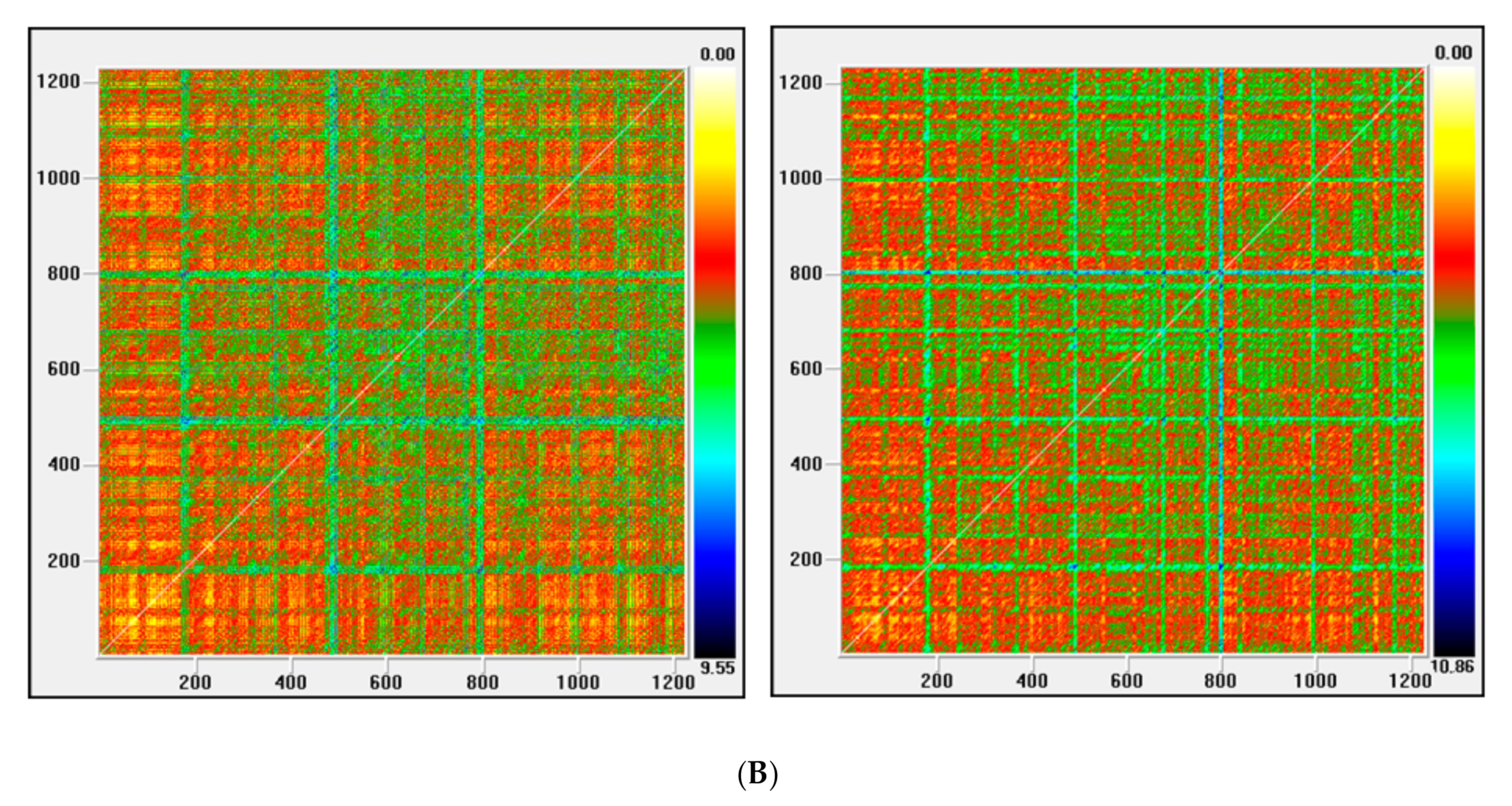In the same way, four methods (correlation dimension, Matilla-Garcia and Ruiz Marin (MGRM) test [38], Lyapunov exponent test, adapted for noisy series [21], and recurrence plots) have been applied to test for chaos. To make the conclusions of this work more robust, besides analyzing the series over the whole period, we have also examined the chaotic behavior over three sub-periods, which were selected by the evolution of volatility.

To this end the following methodology is applied to all time series [32]. First, to evaluate stationarity of the BDI series, unit root tests were performed. Once it had been established that BDI series was I(1), the analysis was carried out on daily returns computed as first difference of the logarithmic price level. Linear dependence was then filtered out of the data by applying autoregressive moving average (ARMA) filters based on the Box–Jenkins methodology [39]. Next, we applied a broad array of procedures to the residuals obtained to detect the existence of nonlinearity. If nonlinear dependence was detected, since linear structures had already been removed using the best fit ARMA model, it was indicative of some type of nonlinear dependence in the returns series resulting from a nonlinear stochastic system or a nonlinear deterministic chaotic system. Stochastic nonlinearity could be due to the presence of a volatility cluster, i.e., large variations tend to group together, which is a common characteristic of financial time series. In such a case, both generalized autoregressive conditional heteroskedasticity (GARCH) [40] and exponential (EGARCH) [41] models were fitted. Afterwards, as a distinctive feature of proposed methodology against published methods, the existence of chaotic structure was examined by a series of robust procedures, including those that are ideally suitable for noisy time series analysis, e.g., Lyapunov exponent test adapted for noisy series, MGRM test based on permutation entropy, and recurrence plots.

Furthermore, the novelty and main contribution of this study lies in the fact that, as far as we know, it is the first time that these robust methods have been applied to detect chaos to such a relevant variable in the world economy, the freight shipping rate. The findings suggest that nonlinearity is present in the underlying process of the BDI although unlike previous studies, we found no sign of chaotic structure. In terms of the benefits of our research for both theory and practice, our results make a significant contribution to shedding light on the underlying behavior and dynamics in shipping rates. In general, our insights should be of great interest to all stakeholders concerned with the shipping industry, including, among others, stevedores, charterers, shipowners, brokers and investment banks.

The rest of the paper is organized as follows. The next section describes the methodological framework applied. The penultimate section presents the data sources used and the main results. Finally, in the final section, we present some conclusions and suggest future lines of research.

2. Methodology

2.1. Methodological Framework

The methodological framework from other research [32,42] has been adopted to study the presence of nonlinearity and chaos. The methods employed herein are presented in

Table 1. Techniques used.

Technique	Reference	Feature Tested
Augmented Dickey Fuller (ADF)	[43]	Stationarity (unit roots)
Phillips–Perron (PP)	[44]	Stationarity (unit roots)
Kwiatkowski–Phillips–Schmidt–Shin (KPSS)	[45]	Stationarity (unit roots)
Keenan	[46]	Nonlinearity
Tsay	[47]	Nonlinearity
White	[48]	Nonlinearity
Brock, Dechert and Sheinkman test-BDS	[49,50]	Independence (iid); Randomness; Nonlinearity
Correlation Dimension	[51]	Chaos
Lyapunov Exponent	[21]	Chaos
MGRM	[38]	Chaos
Recurrence Plots	[52]	Chaos

Note: MGRM stands for the test proposed by Matilla-Garcia and Ruiz Marin [38]. Source: [32] and own work.

, and their main characteristics are described below.

Firstly, we define linear and nonlinear series as elsewhere [32]. A stochastic process ($X_t, t\in T$) is said to be a linear process if for every $t\in T$ $X_t=\sum _{j=0}^{\infty }{\beta }_j{ϵ}_{t-j}$ where $a_0$ = 1, ${ϵ}_t, t\in T$ is a process of independent and identically-distributed random variables (iid) with $E\left[X_t\right]=0, E\left[X_t^2\right]={\sigma }^2$ and $\sum _{j=0}^{\infty }\left|{\beta }_j\right|<\infty$. If a process does not satisfy this condition, then is said to be nonlinear.

The methodological framework includes the following steps.

(i)

Stationarity testing

Stationarity was studied by means of three different techniques (Table 1). Specifically, the Augmented Dickey Fuller test (ADF) [43], Phillips–Perron test (PP) [44] and Kwiatkowski–Phillips–Schmidt–Shin test (KPSS) [45] are applied to time series.

In first instance, once it was tested that each of the four series considered was not stationary, we obtained the log-returns (from now on returns) from each series defined as $\ln \left(R_t\right)=\ln \left(X_t\right)-\ln \left(X_{t-1}\right)$ such that $X_t$ is the time series data at time t. This new series called “return” has important properties such as stationarity. This property is essential, since it is a prerequisite in a large percentage of modelling techniques and in the methods that will be used for the analysis of nonlinearity or chaotic behavior.

(ii)

Linear modelling

Next, ARMA filters were applied to remove the linear dependence present in the return series. The specific model is chosen as the ARMA (p,q) model which presents the lowest value according to the Schwarz information criterion [53]. Following the process described by Barkoulas et al. [54], the residuals were studied. If the residuals were correlated, the order of the ARMA model was increased, by increasing the magnitude of p and q. Once the optimal linear model was determined, the residuals were extracted from it. The new residuals were called the ARMA series.

(iii)

Nonlinearity testing

We used several methods to supplement the limitations of each one. We applied (Table 1): Keenan’s test [46], Tsay’s test [47], White’s test [48] and BDS [49,50].

Before describing the main characteristics of the methods employed in this research, it is worth explaining the process of reconstructing the state space, as well as the concept of attractor.

Following [54], the concept of attractor is defined as follows. Given a discrete dynamic system of the type:

$$x_t=F\left(x_{t-1}\right),x\in R^n$$

(1)

such that P an open subset of $R^n$ and $F:P\to R^n$ is a function [55]; a closed invariant set $A\subset P$ is an attracting limit set of $P$ if there is an open neighborhood $Q$ of $A$, such that the limit set of iterates is $A$, $\forall xϵQ$ when $t\to \infty$.

Empirically, a time series of scalar observations $x_t$, representing the multidimensional system of Equation (1), is usually observed. Using Takens’ embedding theorem [56] it is feasible to recover the dynamics of the system (i.e., the original trajectory) from the observed $x_t$ time series. An m-dimensional vector is defined from $x_t$, and constructed as follows:

$$X_t^m=\left(x_t,\cdots .,x_{t+m-1}\right)=\left(g\left(x_t\right).,g\left(F^{m-1}\left(x_t\right)\right)\right)\equiv J_m$$

(2)

where $F^{m-1}$ means that $F$ is applied a total number of m − 1 times to itself. Thus, our goal is to reconstruct the state dimension space by expanding the one-dimensional signal $x_t$ into an m-dimensional phase space such that each observation in the signal $x_t$ is substituted by the corresponding vector $X_t^m$ in Equation (2). Takens’ embedding theorem states that for each pair $\left(F,g\right)$ the map $J_m: R^n\to R^m$ will be an embedding for $m\ge 2n+1$. If the embedding dimension $m$ is of sufficiently large size with respect to the attractor dimension, Takens’ theorem ensures that a diffeomorphism exists between the original and the reconstructed attractor. In summary, according to the above theorem it can be concluded that both attractors represent the same dynamical system in different coordinate systems if $m\ge 2n+1$.

Nonlinearity tests used in this research are well known in the literature. Thus, only the main features of the BDS method, which has statistical power for detecting nonlinearity and other types of data dependence [21], are presented here. Interestingly, the BDS test can be used to test for nonlinearity if linear structure is removed from the series by fitting an ARMA model. Indeed, if the test is performed on the residuals from a linear model (ARMA process), rejection of the null hypothesis (iid) will denote the presence of linear dependence in the series. The BDS test is constructed as follows [49,50]. Consider a time series ${\left\{x_t\right\}}_{t=1}^T.$ According to Takens’ theorem it is possible to reconstruct the state space from $x_t$. The method of delays is used for reconstruction. Thus, the reconstructed state vector or m-history is $X_t^m=\left(x_t,x_{t+\tau },\cdots .,x_{t+\left(m-1\right)\tau }\right)$ where $\tau$ is the lag or reconstruction delay, and m is the embedding dimension of the reconstructed space. The reconstructed trajectory, X, of N m-dimensional vectors $X_t^m$ can be expressed as a N x m matrix with $N=T-\left(m-1\right)\tau$.

Under the null hypothesis, the BDS statistic is derived using the correlation integral, which measures how many times the temporal patterns in the data are recurrent.

$$V\left(T,m,\epsilon \right)=\sqrt{N}\frac{C\left(T,m,\epsilon \right)-C{\left(T,1,\epsilon \right)}^m}{\widehat{\sigma }\left(T,m,\epsilon \right)}$$

(3)

being $C\left(T,m,\epsilon \right)$ the correlation integral which can be stated as:

$$C\left(T,m,\epsilon \right)=\frac{2}{N\left(N-1\right)}{\displaystyle \sum }_{t<s}H\left\{ϵ-||X_t^m-X_s^m||{}_{ }\right\}$$

(4)

where ‖.‖, m and H represent a norm operator, the embedding dimension and the Heaviside function, respectively.

The correlation integral asymptotically follows a standard normal distribution. $\widehat{\sigma }\left(T,m,\epsilon \right)$ is the standard sample deviation of $C\left(T,m,\epsilon \right)-C{\left(T,1,\epsilon \right)}^m$. Assuming a time series as iid, BDS tests for the null hypothesis that $C\left(T,m,\epsilon \right)=C{\left(T,1,\epsilon \right)}^m$, which is tantamount to the null hypothesis of iid versus an undefined alternative [1].

(iv)

Volatility modelling

In the case of identifying the existence of nonlinear dependence in the residual series from ARMA models, it could be due to the existence of a volatility cluster. To corroborate this hypothesis, conditional variance is modeled by fitting ARCH-type models (GARCH and EGARCH). The selection of the best model is carried out using the same method that was employed for the ARMA model. Once both types of model have been estimated, their standardized residuals are obtained from their conditional standard deviations (hereafter GARCH and EGARCH series). The techniques for detecting the existence of nonlinearity mentioned above are applied to these new GARCH and EGARCH series to contrast whether all the nonlinear dependence has been removed by the process performed.

2.2. Tools to Detect Chaotic Regime

Below, we describe the main characteristics of the tools used for detecting a chaotic regime.

2.2.1. Correlation Dimension

Fractal dimension represents a measure for the level of complexity in the chaotic attractor [1]. This measure has the property of remaining unaltered by the state space reconstruction process. A characteristic of chaotic systems lies in the fact that the fractal dimension is not an integer value [1]. Therefore, estimation of this parameter can be used as a test to detect the presence of chaos. Among the various algorithms for estimating the fractal dimension, the Grassberger and Procaccia algorithm [51] for obtaining the correlation dimension has practical advantages due to its ease of implementation. In fact, with this correlation dimension method, we can distinguish stochastic series from chaotic series [29].

Analogously to the BDS test, this method is also based on the reconstruction of the state space from the observed series and on the correlation integral. Briefly, let ${\left\{x_t\right\}}_{t=1}^T$ be a time series and the sequence of $N=T-m+1$ m-dimensional vectors or m-histories derived from it, $X_t^m=\left(x_t,\cdots ,x_{t+m-1}\right)$ that yields the reconstructed series. The Grassberger and Procaccia algorithm [51] is employed to compute the dimension of the reconstructed attractor. The method relies on the correlation integral which is defined as follows:

$$C\left(ϵ\right)=\frac{2}{N\left(N-1\right)}{\displaystyle \sum }_{t<s}H\left\{ϵ-||X_t^m-X_s^m||{}_{ }\right\}$$

(5)

where m, ‖.‖ and H represent, respectively, the embedding dimension, norm operator and the Heaviside function.

To determine the correlation dimension, it is necessary to determine how $C_{ }\left(\epsilon \right)$ varies as ϵ varies. As the value ϵ rises, the value of $C_{ }\left(\epsilon \right)$ increases due to the greater number of nearby points to include. Grassberger and Procaccia [51] proved that in the case where ε is small enough, $C_{ }\left(\epsilon \right)$ may be well-approximated by $C_{ }\left(\epsilon \right)~{\epsilon }^v$. In other words, when ε→0, $C_{ }\left(\epsilon \right)$ grows at rate $v$. The estimate of $v$ when $m\to \infty$, provides the correlation dimension (CD). In practice, the CD of a dynamic system is determined by estimating the slope of the regression of ${\ln }_{ }{C}_{ }\left(\epsilon \right)$ versus log ϵ and an intercept for small values of $\epsilon$, and depends on the chosen embedding dimension.

In the case where the data are purely stochastic, the value of the correlation dimension will be equal to m for all values of m. If the series is deterministic in nature, the estimated slope will plateau at a point, not rising as m rises. This level of “saturation” of the slope is precisely equal to the estimated correlation dimension for the underlying process.

2.2.2. Lyapunov Exponent

Sensitivity to initial conditions is widely recognized as a core feature of chaos. A checkable quantitative criterion for the sensitivity to initial conditions can be given by the so-called Lyapunov exponents [57]. They calculate the rate of divergence of closely spaced trajectories whose initial conditions only diverge in an infinitesimal amount. LE is one of the most widely used methods to investigate the existence of chaos in time series [23]. The largest Lyapunov exponent can be employed to gauge the separating rate of nearby trajectories and estimate the level of chaotic structure that is present in a nonlinear dynamic system [58]. Under certain conditions, the sign of the coefficient or exponent is a signal of the presence of chaos in the studied series [57]. Specifically, our attention is restricted to systems with bounded metrics, or closed, bounded invariant subsets of unbounded systems. For systems with bounded fluctuations, if the Lyapunov exponent is positive, the orbit exhibits sensitive dependence on initial conditions, and this is a necessary condition of chaotic behaviour [59]. In summary, as Nychka et al. [60] and Bask et al. [61] pointed out, a bounded system with a positive Lyapunov exponent is an operational definition of chaotic behavior in nonlinear dynamic systems that appear to have random and unpredictable behavior.

There are many algorithms in the literature for the estimation of this coefficient. The algorithm proposed by BenSaïda and Litimi [21] is followed in this research. Specifically, it has been empirically proven that this methodology to determine the Lyapunov exponent (λ) is the one that behaves best for noisy series [62]. Indeed, literature shows that there are two main types of technique, which are founded on the reconstruction of the spatial state by means of delay coordinate embedding approaches, to estimate λ from experimental data. Direct methods are based on the computation of the divergence growth rate between two trajectories with an infinitesimal difference in their initial conditions [63]. One of the relevant limitations of this method is that it is sensitive to both sample size and level of noise in the data [64]. By contrast, the Jacobian-based approach can provide robust estimates of Lyapunov exponents despite the existence of noise [65,66]. The Jacobian method relies on non-parametric regression to estimating the Jacobians and λ. However, as for a scalar time series, the map that triggers the process is generally not known; the Jacobian matrix cannot be obtained and, therefore, the Lyapunov exponent cannot be determined. To do so, it is necessary to approach the unknown chaotic map by means of a given function. McCaffrey et al. [65] compared the results of various approaches: radial basis functions, neural networks, thin-plate splines, and projection search. On the basis of their simulations, neural network behaved as the best regression method for the case of chaotic systems with noise. In this line, Bailey et al. [66] suggested a regression method that involves using neural networks. Simulation results for a Henon system containing noise showed that neural network regression method provides accurate estimates for the Lyapunov exponent.

Following [21], the methodology comprises the following steps: consider a time series ${\left\{x_t\right\}}_{t=1}^T$. A noisy chaotic system can be expressed as follows:

$$X_t=f\left(x_{t-\tau },x_{t-2\tau },\cdots , x_{t-m\tau }\right)+{\epsilon }_t$$

(6)

where t is the time script and m, τ, ${\epsilon }_t$ and f represent the embedding dimension, the time delay, noise added to the series and an unknown chaotic map, respectively. The Lyapunov exponent (LE) is set as:

$$\widehat{{\lambda }}=\frac{1}{2M}\ln \left(v_1\right)$$

(7)

where $M\le T$ is the “block-length” or number of equally spaced evaluation points that are used to calculate the Lyapunov exponent and $v_1$ is the largest eigenvalue of the matrix ${\left(T_M{U}_0\right)}^{\prime }\left(T_M{U}_0\right),$ being $T_M=\prod _{t=1}^{M-1}{J}_{M-t},$ $J_t$ the Jacobian matrix of the chaotic map and $U_0={\left(1, 0, \cdots , 0\right)}^{\prime }$. Since we usually do not know the chaotic map F, the Jacobian matrix could not be estimated. Therefore, it is necessary to approximate the unknown chaotic map by the appropriate function.

As in [18], a neural network function, with a q-dimensional hidden layer and a hyperbolic tangent function as the activation function, is adopted. It is estimated by the nonlinear least squares method, varying m from 1 to 8, in order to subsequently compute the LE spectrum. Thus, the chaotic process is estimated by using the equation below:

$$x_t\approx {\alpha }_0+{\displaystyle \sum }_{j=1}^q{\alpha }_j\tan h\left({\beta }_{o,j}+{\displaystyle \sum }_{i=1}^m{\beta }_{i,j}{x}_{t-i\tau }\right)+{\epsilon }_t$$

(8)

The triplet (τ, m, q) defines the complexity associated with the process and is selected as the one that determines the largest value for λ. Then, from the asymptotic distribution of λ, the test for the presence of chaos is constructed [63].

2.2.3. Matilla-Garcia and Ruiz Marin (MGRM) Test

The MGRM Test [38] is a test for the deterministic process as opposed to the stochastic one which is rooted in symbolic dynamics and entropy. In particular, the concept of permutation entropy, which has its origin in symbolic dynamics, is the foundation of the MGRM test. The basic idea of symbolic dynamics consists of partitioning the phase space into a finite set of regions and to assign an alphabetic symbol to each region. A relevant property of symbolic dynamics is that essential features of the underlying dynamics, namely deterministic or stochastic nature or complexity, are preserved. Likewise, entropy provides an insight into the unpredictability of the system under study, which is a key feature of complex systems.

In the first instance the notation is introduced: let ${\left\{x_t\right\}}_{t\in T}$ be a stationary time series, ${\left\{x_t\right\}}_{t\in I}$ an observation with $I=\left\{1,\cdots ,T\right\}$ and m the embedding dimension with $m\ge 2$. We will define the ordinal patterns for “m”. As we already know, the scalar time series can be embedded in an m-dimensional space as follows: $x_m\left(t\right)=\left(x_t,x_{t+1},\cdots ,x_{t+\left(m-1\right)}\right) \mathrm{for} t\in T.$ For a given time value t, the ordinal pattern corresponding to embedding dimension m is set to be the unique permutation ${\pi }_m\left(t\right)\equiv \left(r_0 r_1\cdots \cdots r_{m-1}\right)$ of the set $\left\{0, 1, . . ., \mathrm{m}-1\right\}$ that satisfies:

$$x_{t+r_0}\le x_{t+r_1}\le \cdots \le x_{t+r_{m-1} }$$

(9)

$$r_{s-1}<r_s \mathrm{if} x=x_{t+r_s }$$

(10)

By means of Equation (9) it is guaranteed that the permutation defined by Equation (10) is unique. Therefore, the vector or m-history $X_m\left(t\right)$ is transformed into a unique symbol ${\pi }_m\left(t\right)$. In fact, ${\pi }_m\left(t\right)$ shows us how the ordering of the times: $t+0<t+1<\cdots <t+\left(m-1\right)$ becomes the order of the correspondent values being analyzed. The core point is to split the state space in which the dynamical process unfolds into a finite number of sets exploiting the time dependent information held in the m-history $X_m\left(t\right)\in R^m$. According to the above definition, the partitions depend on how the ordinal structure corresponds to the m-history is. In particular, ${\pi }_m\left(t\right)={\pi }_m\left(s\right), s\ne t$, if and only if for all $k,I ϵ \left\{0,1,\cdots ,m-1\right\}$ with $k\ne I$ it holds that $x_{t+1}\le x_{t+k}\leftrightarrow x_{s+1}\le x_{s+k}.$

In general, given a time series ${\left\{x_t\right\}}_{t\in T}$, all m! permutations of order m are taken as potential order types of m distinct numbers. Then, for an embedding dimension parameter m, the relative frequency or unconditional success probability $p\left(\pi \right)$ of each symbol or permutation $\pi$ can be set as:

$$p\left(\pi \right)=\frac{card\left\{t | 0 \le t \le T-\left(m-1\right), Y_m\left(t\right) has type \pi \right\}}{T-m+1}$$

(11)

Given an embedding dimension $m\ge 2$, Shannon entropy that stands for the m! distinct symbols, is defined as follows:

$$h\left(m\right)=-{\displaystyle \sum }_{i=1}^{m!}p\left({\pi }_i\right)\log p\left({\pi }_i\right)$$

(12)

The test is constructed as follows: Let m be embedding dimension and T be the number of observations and fix $w,k\in \mathbb{N}$ such that $w=\frac{m!}{k}$. Next, the subsets $W_j$ that must verify $W_1\subseteq W_2\subseteq \cdots \subseteq W_n$ in the following way $W_j=W_{j-1}\cup \left\{ w \mathrm{symbols} \mathrm{chosen} \mathrm{at} \mathrm{random} \mathrm{in} S_m \backslash W_{j-1}\right\}$ for j = 2, …, k are constructed.

Subsequently the next permutation entropy’s function is calculated as:

$$h^{W_j}\left(m\right)=-{\displaystyle \sum }_{{\pi }_j\in w_j}p\left(\pi \right)\log p\left(\pi \right)$$

(13)

When analyzing the permutation entropy’s function values, it is possible to distinguish and identify deterministic systems. In this process no additional information is obtained by an increase in the number of symbols considered. In contrast, in non-deterministic process, this information or complexity is increased.

This latter property is tested in the following way: Let $d{h}^{W_j}\left(m\right)$ be the $h^{W_j}\left(m\right)$ slope:

$$d{h}^{W_j}\left(m\right)=\frac{h^{W_{j+1}}\left(m\right)-h^{W_j}\left(m\right)}{\log \left(\frac{j+1}{j}\right)}$$

(14)

When considering random process, the numerical slope of permutation entropy will rise with log(jw), while this will not be the case for chaotic or regular processes.

The property described above that identifies deterministic systems $h^{W_j}\left(m\right)$ is tested by carrying out the following regression:

$$d{h}^{W_j}\left(m\right)={\alpha }_0+{\alpha }_{1}j+{\epsilon }_j for j=1,2,\cdots , k-1$$

(15)

where ${\epsilon }_j$ is white noise. As a result, the estimated parameter ${\widehat{\alpha }}_1$ can be employed to assess how $d{h}^{W_j}\left(m\right)$ scales with j. In mathematic notation, the test is the following one:

$$\begin{array}{c}{H}_0\equiv {\alpha }_1=0\\ H_1\equiv {\alpha }_1>0\end{array}$$

(16)

Indeed, regression (15) can be considered as a simple symbol-trend model. The same as for the basic time-trend model, the ordinary least squares estimate ${\widehat{\alpha }}_1$ is such that the standard t-test of H₀: ${\widehat{\alpha }}_1=0$ is asymptotically valid. If the coefficient obtained is null, then the series is deterministic; otherwise (greater than 0), it is stochastic [38].

2.2.4. Recurrence Plots

A recurrence plot (RP) reveals the existence of recurrent and intermittent patterns in time series. First proposed by Ekmann et al. [52,67], it has been widely applied in the characterization of dynamic systems. This topological method shows the hidden structures of time series from a qualitative perspective. The plots are constructed by assuming mutual distances that belong to the same path in the reconstructed state space [42]. The construction is done as follows.

Let m be the embedding dimension and $X_t^m$ the vector m-dimensional in the reconstructed state space at time t ranging from 1 to k. The recurrence matrix is generated by comparing each embedded vector $X_i^m$ with the other $X_j^m$. A point is drawn if this comparison is less than a value ε for a specific distance. That is, if the condition is met: $||X_i^m-{\mathrm{X}}_{\mathrm{j}}^{\mathrm{m}}||<\epsilon$. Recurrence of a state between $\mathrm{t}=\mathrm{i}$ and $\mathrm{t}=\mathrm{j}$ occurs when ${\mathrm{X}}_{\mathrm{j}}^{\mathrm{m}}$ is close enough to $X_i^m$. The RP can, therefore, show which vectors are close together and which are far apart.

The diagonal structures of the RP define the extent to which one part of the path is relatively near to another at a distinct time. For the case of a deterministic chaos system, short lines parallel to the main diagonal are visible. However, in stochastic systems, short line segments are missing, and uniformly distributed points are displayed.

This technique is independent of some constraints such as sample size, noise, and stationarity [1]. It also provides additional information about the structure of the attractor, since the plot preserves the temporal order of the series, allowing the place and periodicity of the periodic orbits to be known.

3. Empirical Results

Applying the methodological framework described above, the main results obtained are shown below.

3.1. Data

The data set corresponds to daily observations of the BDI comprising the period between 1 January 1990 until 1 July 2013 and was obtained from the Bloomberg (http://www.bloomberg.com/ (accessed on 26 May 2014) and Baltic Exchange Web sites (http://www.balticexchange.com/ (accessed on 26 May 2014)). In addition, as a complement to the above and after checking that the initial series had periods of different volatility, it was decided to divide the original series into three new series, taking into account the following sub-periods: (i) BDI1 series (from 1 January 1990 until 31 December 2002); (ii) BDI2 series (from 1 January 2003 until 31 December 2007) and (iii) BDI3 series (from 1 January 2008 until 1 July 2013).

Figure 1 shows that the BDI remained relatively stable, following a course lacking in significant shocks until 2003. Then, there was a dramatic increase in volatility, adopting a behavior that mimics financial bubbles. After the ocean freight boom (2005–2006 period), on 20 May 2008, the BDI attained its maximum value (11,793) since its introduction in 1985. However, it immediately decreased 94% during the period of May to December 2008, in the midst of the complete turmoil of the financial crisis. It was not until 5 December 2008, that it registered a value of 663 points, corresponding to its minimum value since 1985. This decrease is partially related to the reduction in demand for global goods that translated into a fall in the demand for transportation and coincides with an increase in the supply due to the deliveries of new ships ordered during the boom period of the global economy.

Table 2. Descriptive statistics.

BDI Series
	Original Series	Returns	ARMA(9,0)	GARCH(1,2)	EGARCH(2,3)
Mean	2283.77	−7.2 × 10−5	4.26 × 10−11	0.0150	0.0078
Standard Deviation	1909	0.0148	0.0084	0.9723	1.0030
Median	1531	−9.3 × 10−5	−0.0001	−0.0191	−0.0282
Minimum	647	−0.1200	−0.0783	−5.8461	−5.4268
Maximum	11,793	0.1400	0.0978	12.6105	7.1285
Skewness Coefficient	2.41	−0.0600	0.3766	1.1198	0.4531
Kurtosis Coefficient	9.21	12.8000	18.5728	15.1364	6.8089
Jarque–Bera Test	14,634.4 *	22,759.8 *	57,559.1 *	36,065.6 *	3629.8 *
N	5692	5691	5683	5683	5683
BDI1 Series
	Original Series	Returns	ARMA(5,0)	GARCH(1,1)	EGARCH(3,1)
Mean	1360.46	2.7 × 10−5	−3 × 10−11	−0.0051	0.0147
Standard Deviation	314.98	0.0072	0.0042	0.9634	1.0022
Median	1353	−0.0006	−0.0001	−0.0399	−0.0152
Minimum	776.00	−0.0390	0.0385	−4.9043	−4.7600
Maximum	2352	0.0430	−0.0280	8.5857	7.1635
Skewness Coefficient	0.4906	0.5870	0.7382	0.6285	0.4990
Kurtosis Coefficient	3.1099	5.9019	11.6736	8.1090	6.8966
Jarque–Bera Test	124.23 *	1248.6 *	9847.4 *	3521.2 *	2058.2 *
N	3059	3058	3053	3053	3053
BDI2 Series
	Original Series	Returns	ARMA(3,0)	GARCH(1,1)	EGARCH(1,1)
Mean	4157.69	0.0013	3.2 × 10−12	−0.0490	−0.0235
Standard Deviation	2028.52	0.0134	0.0066	0.9611	0.9997
Median	4038.50	0.0017	−0.0002	−0.0885	−0.0668
Minimum	1530	−0.1200	−0.0444	−5.3013	−4.9095
Maximum	11,793	−0.1400	0.0855	4.2758	4.1532
Skewness Coefficient	1.4447	0.2819	1.5200	0.0166	0.0341
Kurtosis Coefficient	5.2447	4.3000	29.8387	4.9490	4.6545
Jarque–Bera Test	690.58 *	100.91 *	37,632	196.0	141.44
N	1238	1238	1238	1238	1238
BDI3 Series
	Original Series	Returns	ARMA(7,0)	GARCH(1,1)	EGARCH(1,1)
Mean	2645.20	−0.0015	−8.90 × 10−11	0.0036	0.0066
Standard Deviation	2427.37	0.0251	0.0142	0.9649	1.0004
Median	1817.50	−0.0019	−0.0006	−0.0603	−0.0600
Minimum	647	−0.1200	−0.0767	−4.3534	−4.5133
Maximum	11,793	0.1370	0.0986	5.8011	6.2652
Skewness Coefficient	1.8980	0.0120	0.2360	0.6857	0.6806
Kurtosis Coefficient	5.9415	6.0840	7.7169	7.1488	7.2499
Jarque–Bera Test	1341.42 *	553.2 *	1307.1	1110.58	1158.3
N	1396	1396	1396	1396	1396

Note: Statistics for the considered time series: original series, return series, residuals of autoregressive moving average (ARMA) process, as well as standardized residuals from generalized autoregressive conditional heteroscedastic (GARCH) model and exponential GARCH (EGARCH) process. Skewness corresponds to Fisher’s skewness coefficient. *: Asterisk denotes significance at the 5% level. N is the number of observations. Source: Own work.

presents the main descriptive statistics of the four series studied. All series show a positive skewness coefficient. Moreover, it can be concluded that the data do not come from a normal distribution, as reflected by the Jarque–Bera test (p-value < 0.05).

3.2. Returns

To evaluate the stationarity of the BDI series, unit root tests are performed [68,69]. Specifically, we examine the stationary property by applying the Augmented Dickey–Fuller test [43], the Phillips–Perron test [44] and the Kwiatkowski–Phillips–Schmidt–Shin contrast [45]. After testing that the four series are not stationary (see

Table 3. Stationarity analysis.

BDI	Original Series	Return Series
1. Augmented Dickey–Fuller Test
Constant	−3.3632 (0.0124)	−18.5200 (0.0000)
Constant and Linear Trend	−3.4880 (0.0407)	−18.5215 (0.0000)
2. Phillips–Perron Test
Constant	−2.7104 (0.0723)	−23.4660 (0.0000)
Constant and Linear Trend	−2.7660 (0.2101)	−23.4661 (0.0000)
3. Kwiatkowski–Phillips–Schmidt–Shin Test
Constant	2.0704	0.0510
Constant and Linear Trend	0.5854	0.0385
BDI1	Original Series	Return Series
1. Augmented Dickey–Fuller Test
Constant	−2.7328 (0.0686)	−16.0082 (0.0000)
Constant and Linear Trend	−2.6569 (0.2549)	−16.0196 (0.0000)
2. Phillips–Perron Test
Constant	−2.2710 (0.1816)	−18.3371 (0.0000)
Constant and Linear Trend	−2.1487 (0.5176)	−18.3492 (0.0000)
3. Kwiatkowski–Phillips–Schmidt–Shin Test
Constant	0.8911	0.0892
Constant and Linear Trend	0.2590	0.0593
BDI2	Original Series	Return Series
1. Augmented Dickey–Fuller Test
Constant	−0.0856 (0.9491)	−13.1635 (0.0000)
Constant and Linear Trend	−0.7875 (0.9653)	−13.1591 (0.0000)
2. Phillips–Perron Test
Constant	−0.2200 (0.9334)	−8.5187 (0.0000)
Constant and Linear Trend	−0.9141 (0.9528)	−8.5131 (0.0000)
3. Kwiatkowski–Phillips–Schmidt–Shin Test
Constant	1.6140	0.1329
Constant and Linear Trend	0.5925	0.1274
BDI3	Original Series	Return series
1. Augmented Dickey–Fuller Test
Constant	−2.5787 (0.0976)	−14.5984 (0.0000)
Constant and Linear Trend	−2.3326 (0.4154)	−14.6130 (0.0000)
2. Phillips–Perron Test
Constant	−2.6358 (0.0860)	−12.2124 (0.0000)
Constant and Linear Trend	−2.6044 (0.2784)	−12.2111 (0.0000)
3. Kwiatkowski–Phillips–Schmidt–Shin Test
Constant	2.3457	0.0690
Constant and Linear Trend	0.3092	0.0385

Note: Augmented Dickey–Fuller p-values correspond to [72] one-sided p-values. For the Phillips–Perron test, lags were based on bandwidth Newey–West using the Bartlett kernel. Critical values for the Kwiatkowski, Phillips, Schmidt and Shin test are 0.463 and 0.146, respectively, for the constant and linear plus linear trend model. Significant values at the 95% confidence level are in bold.

), the returns from each series were obtained by considering the logarithms of the ratio of two consecutives prices. Figure 2 shows the time development of the returns. The peak in 1999 matches with the methodological change implemented in the index definition. Return series shows a negative skewness coefficient, that is, the distribution is left-skewed, implying that upward jumps of larger size are less frequent than downward jumps of smaller size, as do financial time series [70]. It is worth noting the high value of the kurtosis coefficient, which implies that large jumps are more likely to happen more frequently than in the normal distribution. This result is not altogether surprising because the BDI series presents similar characteristics to financial series, as previously stated [71].

In the evolution of the return series corresponding to each of the three sub-periods, two peaks corresponding to the 1997 Asian crisis (BDI1 returns series) and the 2008 world recession (BDI3 returns series) are displayed. The three series present a positive skewness coefficient and an excess of kurtosis, with the latter reaching a greater magnitude in the third series (BDI3 returns series). According to the results from the Augmented Dickey–Fuller, Philips–Perron and KPSS tests, all the three returns series are stationary (Table 3).

3.3. Linear Dependence

As some methodology (for example the BDS test) is not robust for the presence of linear relationships, the linear dependence was removed using ARMA models. Following the criterion described by [54], the best ARMA model was selected for each series (

Table 4. Classes of models applied to each series.

Series	Linear Model	Nonlinear Model
	[ARMA]	[GARCH]	[EGARCH]
BDI	ARMA(9,0)	GARCH(1,2)	EGARCH(2,3)
BDI1	ARMA(5,0)	GARCH(1,1)	EGARCH(3,1)
BDI2	ARMA(3,0)	GARCH(1,1)	EGARCH(1,1)
BDI3	ARMA(7,0)	GARCH(1,1)	EGARCH(1,1)

). The selected fitted models for each of the series (ARMA(9,0); ARMA(5,0); ARMA(3,0) and ARMA(7,0)), for the series BDI, BDI1, BDI2 and BDI3 respectively, are shown in Table 4 that displays all the models fitted in this research. Details of each model are presented in Appendix A (Tables A1, A4, A7 and A10). According to the results from the Augmented Dickey–Fuller, Philips–Perron and KPSS tests applied on the residuals of the selected model, and shown in Table 3, all the residuals series (ARMA) are stationary.

3.4. Nonlinear Dependence

Next, Keenan, Tsay, White and BDS methods were used to study nonlinearity. The principal advantage of using a broad set of instruments is to obtain the most information possible about the nature of the series, since to date none of the methods has proved successful in detecting all types of dependence. Nevertheless, some tests, such as the BDS or White are more efficient in detecting dependency [3]. Results by applying Keenan, Tsay and White methods are exhibited in Appendix B (

Table A13. Nonlinearity tests (BDI series).

BDI
Test	Returns	ARMA(9,0)	GARCH(1,2)	EGARCH(2,3)
Keenan	21.3281 [9]	0.0009 [0]	1.8963 [1]	0.4427 [0]
	3.956 × 10−6	0.9766	0.1685	0.5058
Tsay	5.354 [9]	0.0296 [0]	3.013 [1]	1.4550 [0]
	7.235 × 10−28	0.9932	0.0826	0.2249
White	70.4337	132.4288	15.2346	32.896
	5.551 × 10−16	<2.2 × 10−16	0.0005	7.583 × 10−8

The first row shows the statistic associated with the test and in brackets, if necessary, the dimension of the model chosen to carry out the corresponding test. The second row shows the p-value. In bold, those values with a p-value < 0.05.

and

Table A14. Nonlinearity tests (subsamples).

BDI1
Test	Returns	ARMA(5,0)	GARCH(1,1)	EGARCH(3,1)
Keenan	11.3067 [5]	2.8761 [26]	2.3620 [5]	0.1159 [0]
	0.0008	0.0901	0.1244	0.7336
Tsay	5.8340 [5]	2.5410 [26]	0.7093 [5]	0.1371 [0]
	4.519 × 10−12	2.978 × 10−39	0.7775	0.9379
White	137.7620	19.134	18.3153	5.1852
	<2.2 × 10−16	7 × 10−5	0.00011	0.07483
BDI2
Test	Returns	ARMA(3,0)	GARCH(1,1)	EGARCH(1,1)
Keenan	6.2973 [3]	0.3993 [0]	1.0558	1.4827
	0.0122	0.5276	0.3044	0.2236
Tsay	7.4420 [3]	0.0887	1.2910 [5]	1.349 [5]
	7.631 × 10−8	0.9663	0.1999	0.1653
White	46.4004	155.3275	3.8903	5.8127
	8.4 × 10−11	<2.2 × 10−16	0.1430	0.0547
BDI3
Test	Returns	ARMA(7,0)	GARCH(1,1)	EGARCH(1,1)
Keenan	8.8210 [7]	0.0006 [0]	0.0158 [0]	0.0011 [0]
	0.0030	0.9806	0.9001	0.9736
Tsay	2.4470 [7]	0.1001 [0]	0.1445 [0]	0.2253
	4.16 × 105	0.9599	0.9332	0.8788
White	20.9735	42.7376	14.3453	9.373
	2.79 × 10−5	5.2 × 10−10	0.0008	0.0092

Note: The first row shows the statistic associated with the test and in brackets, if necessary, the dimension of the model chosen to carry out the corresponding test. The second row shows the p-value.

).

The BDS test was applied once the linear dependence was eliminated, as previously suggested by [73]. In this way the BDS test served as an indirect method of analyzing nonlinearity: if it rejected the null hypothesis, then the series was proven to be nonlinear. This procedure is theoretically feasible, since the calculations on the residuals of an autoregressive model do not lose the relevant information derived from the original series if the latter comes from a nonlinear chaotic system [73]. The BDS test is applied taking into account different embedding dimensions (range: 2–9). The results are presented in Appendix B (

Table A15. BDS test results for ARMA(9,0) series.

ϵ	m
	0.5	σ	1.5σ	2σ
2	34.5547	36.2656	34.4998	31.6277
	0.0000	0.0000	0.0000	0.0000
3	44.8132	42.6536	38.6800	34.5903
	0.0000	0.0000	0.0000	0.0000
4	55.4024	47.5911	41.0281	35.6805
	0.0000	0.0000	0.0000	0.0000
5	69.2478	52.7536	43.2854	36.6743
	0.0000	0.0000	0.0000	0.0000
6	88.9560	58.5848	45.3847	37.4547
	0.0000	0.0000	0.0000	0.0000
7	116.3227	65.4426	47.5975	38.2830
	0.0000	0.0000	0.0000	0.0000
8	155.9435	73.6903	49.9559	39.1370
	0.0000	0.0000	0.0000	0.0000

Note: The first row shows the statistic associated with the test. The second row shows the p-value. Values with a p-value less than the significance level 0.05 are shown in bold. m is the embedding dimension and ϵ is the distance expressed by the number of standard deviations of the data: (0.5−2)*σ.

and

Table A26. BDS test results for EGARCH(1,1) series.

ϵ	m
	0.5σ	σ	1.5σ	2σ
2	3.6584	3.3261	2.2337	0.8868
	0.0003	0.0009	0.0255	0.3752
3	4.2227	3.5075	2.3168	0.8348
	0.0000	0.0005	0.0205	0.4038
4	4.6801	3.6679	2.4175	1.0168
	0.0000	0.0002	0.0156	0.3092
5	5.6338	4.0064	2.5585	1.0689
	0.0000	0.0001	0.0105	0.2851
6	6.8257	4.3979	2.6516	1.0627
	0.0000	0.0000	0.0080	0.2879
7	7.4175	4.6802	2.7816	1.1140
	0.0000	0.0000	0.0054	0.2653
8	8.8002	5.0099	2.8932	1.2049
	0.0000	0.0000	0.0038	0.2282

Note: The first row shows the statistic associated with the test. The second row shows the p-value. Values with a p-value less than the significance level 0.05 are shown in bold. m is the embedding dimension and ϵ is the distance expressed by the number of standard deviations of the data: (0.5−2)*σ.

).

Table 5. Summary of results for the nonlinear analysis.

BDI Series
Test	Ho	Returns	ARMA(9,0)	GARCH(1,2)	EGARCH(2,3)
Keenan	La	R	NR	NR	NR
Tsay	La	R	NR	NR	NR
White	La	R	R	R	R
BDS	Lb	-	R	Mixture	R
BDI1 Series
Test	Ho	Returns	ARMA(5,0)	GARCH(1,1)	EGARCH(3,1)
Keenan	La	R	NR	NR	NR
Tsay	La	R	R	NR	NR
White	La	R	R	R	NR
BDS	Lb	-	R	NR	NR
BDI2 Series
Test	Ho	Returns	ARMA(3,0)	GARCH(1,1)	EGARCH(1,1)
Keenan	La	R	NR	NR	NR
Tsay	La	R	NR	NR	NR
White	La	R	R	NR	R
BDS	Lb	-	R	NR	NR
BDI3 Series
Test	Ho	Returns	ARMA(7,0)	GARCH(1,1)	EGARCH(1,1)
Keenan	La	R	NR	NR	NR
Tsay	La	R	NR	NR	NR
White	La	R	R	R	R
BDS	Lb	-	R	R	R

Ho: Null hypothesis. La: Linear in mean. Lb: This test can be applied as a linear test once the linear dependence has been eliminated. R represents that null hypothesis is rejected; NR represents that null hypothesis is not rejected. Mixture represents that the test reported no clear results.

presents a summary of results for the nonlinear analysis. Results from all procedures suggest the existence of nonlinearity in all the four returns series. Likewise, if the results of the tests with the highest power are considered (White and BDS), all ARMA series seem to present some type of dependence. In particular, the BDS test shows significant results in all ARMA series for the different embedding dimensions and ϵ values being considered.

3.5. Volatility Clustering

The next step consists of modelling the conditional variance by fitting ARCH family models (GARCH and EGARCH). In first instance, the best GARCH (p,q) model was selected so as to adhere to the previously described criterion [54]. After fitting each model, standardized residuals were obtained (from now on GARCH and EGARCH series). Unlike GARCH models, EGARCH models can be used to estimate conditional variance, taking into consideration the sign of the past period’s innovation. The asymmetric response in the conditional variance is successfully captured by this class of model and, therefore, they are well suited candidates for modeling financial series. The chosen models were EGARCH (2,3) and EGARCH (3,1) for BDI and BDI1 series, respectively, and EGARCH (1,1) for both BDI2 and BDI3 series (Table 4). Details of each model are presented in Appendix A (

Table A2. GARCH(1,2) model for the BDI series.

	Coefficient	Standard Deviation	T Statistic	p-Value
C	6.97 × 10−6	3.62 × 10−7	19.2551	0.0000
RESID(−1)2	0.6010	0.0258	23.2663	0.0000
GARCH(−1)	0.1638	0.0257	6.3814	0.0000
GARCH(−2)	0.2473	0.0181	13.6303	0.0000

The linear model has been previously presented.

,

Table A3. EGARCH (2,3) model for the BDI series.

	Coefficient	Standard Deviation	T Statistic	p-Value
C(1)	−0.0163	0.0021	−7.8149	0.0000
C(2)	0.4959	0.0160	30.9642	0.0000
C(3)	−0.4772	0.0156	−30.5252	0.0000
C(4)	−0.0063	0.0010	−6.2697	0.0000
C(5)	1.4776	0.0087	170.1538	0.0000
C(6)	−0.2187	0.0003	−675.2090	0.0000
C(7)	−0.2592	0.0084	−30.8526	0.0000

The linear model has been previously presented.

,

Table A4. ARMA(5,0) model for the BDI1 series.

	Coefficient	Standard Deviation	T Statistic	p-Value
C	9.98 × 10−6	0.0004	0.0248	0.9802
AR(1)	0.7416	0.0181	40.9841	0.0000
AR(2)	0.0749	0.0225	3.3237	0.0009
AR(3)	0.0232	0.0226	1.0277	0.3042
AR(4)	0.0123	0.0225	0.5750	0.5654
AR(5)	−0.0439	0.0181	−2.4287	0.0152

,

Table A5. GARCH(1,1) model for the BDI1 series.

	Coefficient	Standard Deviation	T Statistic	p-Value
C	1.46 × 10−6	2.06 × 10−7	7.07427	0.0000
RESID(−1)2	0.2435	0.0139	17.5775	0.0000
GARCH(−1)	0.7246	0.0111	65.5549	0.0000

The linear model has been previously presented.

,

Table A6. EGARCH(3,1) model for the BDI1 series.

	Coefficient	Standard Deviation	T Statistic	p-Value
C(1)	−0.1837	0.0213	−8.6396	0.0000
C(2)	0.4100	0.0235	17.4340	0.0000
C(3)	−0.2875	0.0324	−8.8699	0.0000
C(4)	0.0061	0.0248	0.2441	0.8072
C(5)	−0.0223	0.0053	−4.2008	0.0000
C(6)	0.9919	0.0016	602.1425	0.0000

The linear model has been previously presented.

,

Table A7. ARMA(3,0) model for BDI2 series.

	Coefficient	Standard Error	T Statistic	p-Value
C	0.0013	0.0009	1.4432	0.1492
AR(1)	1.0485	0.0282	37.1806	0.0000
AR(2)	−0.1129	0.0409	−2.7589	0.0059
AR(3)	−0.1367	0.0282	−4.8422	0.0000

,

Table A8. GARCH(1,1) model for BDI2 series.

	Coefficient	Standard Deviation	T Statistic	p-Value
C	6.1 × 10−6	8.67 × 10−7	6.9744	0.0000
RESID(−1)2	0.5065	0.0440	11.4983	0.0000
GARCH(−1)	0.4587	0.0289	15.8957	0.0000

The linear model has been previously presented.

,

Table A9. EGARCH(1,1) model for BDI2 series.

	Coefficient	Standard Deviation	T Statistic	p-Value
C(5)	−1.8485	0.2025	−9.1301	0.0000
C(6)	0.5542	0.0346	16.0138	0.0000
C(7)	−0.0221	0.0235	−0.9397	0.3474
C(8)	0.8631	0.0183	47.1652	0.0000

The linear model has been previously presented.

,

Table A11. GARCH(1,1) model for BDI3 series.

	Coefficient	Standard Deviation	T Statistic	p-Value
C	4.83 × 10−5	3.85 × 10−6	12.5413	0.0000
RESID(−1) 2	0.3962	0.0296	13.4044	0.0000
GARCH(−1)	0.4545	0.0301	15.1062	0.0000

The linear model has been previously presented.

and

Table A12. EGARCH model (1,1) for BDI3 series.

	Coefficient	Standard Deviation	T Statistic	p-Value
C(1)	−3.1877	0.2500	−12.7520	0.0000
C(2)	0.5820	0.0365	15.9424	0.0000
C(3)	0.0454	0.0241	1.8861	0.0593
C(4)	0.6813	0.0270	25.3200	0.0000

The linear model has been previously presented.

). The standardized residuals of all the series are less leptokurtic than those obtained from ARMA models (Table 2).

Since nonlinearity is a necessary, but not sufficient, condition for chaotic behavior, its existence was first analyzed in residuals of the volatility models (Table 5 and Table A13, Table A14, Table A15,

Table A16. BDS test results for GARCH(1,2) series.

ϵ	m
	0.5σ	σ	1.5σ	2σ
2	0.3935	0.6491	0.2717	−0.4000
	0.6939	0.5163	0.7858	0.6891
3	2.7572	2.6768	1.9576	0.9089
	0.0058	0.0074	0.0503	0.3634
4	3.3252	3.1852	2.2457	0.9689
	0.0009	0.0014	0.0247	0.3326
5	4.5027	4.1190	2.8631	1.3183
	0.0000	0.0000	0.0042	0.1874
6	5.7009	4.9818	3.2556	1.4138
	0.0000	0.0000	0.0011	0.1574
7	7.1800	5.8674	3.7291	1.6037
	0.0000	0.0000	0.0002	0.1088
8	9.0922	6.8478	4.2720	1.8624
	0.0000	0.0000	0.0000	0.0625

Note: The first row shows the statistic associated with the test. The second row shows the p-value. Values with a p-value less than the significance level 0.05 are shown in bold. m is the embedding dimension and ϵ is the distance expressed by the number of standard deviations of the data: (0.5–2)*σ.

,

Table A17. BDS test results for EGARCH(2,3) series.

ϵ	m
	0.5σ	σ	1.5σ	2σ
2	2.5457	3.0959	3.2182	2.6562
	0.0109	0.0020	0.0013	0.0079
3	3.0470	3.6883	3.7721	3.1753
	0.0023	0.0002	0.0002	0.0015
4	2.6107	3.4351	3.4530	2.9061
	0.0090	0.0006	0.0006	0.0037
5	2.7139	3.4367	3.3606	2.8156
	0.0066	0.0006	0.0008	0.0049
6	2.8467	3.4401	3.2364	2.6656
	0.0044	0.0006	0.0012	0.0077
7	2.6044	3.3420	3.0751	2.4991
	0.0092	0.0008	0.0021	0.0125
8	3.1909	3.2643	2.9028	2.3941
	0.0014	0.0011	0.0037	0.0167

Note: The first row shows the statistic associated with the test. The second row shows the p-value. Values with a p-value less than the significance level 0.05 are shown in bold. m is the embedding dimension and ϵ is the distance expressed by the number of standard deviations of the data: (0.5–2)*σ.

,

Table A18. BDS test results for ARMA(5,0) series.

ϵ	m
	0.5σ	σ	1.5σ	2σ
2	0.7586	0.8973	0.8976	0.5702
	0.0000	0.0000	0.0000	0.0000
3	1.8268	1.8194	1.6749	1.1824
	0.0000	0.0000	0.0000	0.0000
4	1.7420	1.9256	1.8692	1.3868
	0.0000	0.0000	0.0000	0.0000
5	1.8758	2.2496	2.1912	1.6989
	0.0000	0.0000	0.0000	0.0000
6	2.0473	2.5956	2.4954	1.9694
	0.0000	0.0000	0.0000	0.0000
7	1.9352	2.7204	2.5835	2.0280
	0.0000	0.0000	0.0000	0.0000
8	1.6852	2.8417	2.6866	2.1696
	0.0000	0.0000	0.0000	0.0000

Note: The first row shows the statistic associated with the test. The second row shows the p-value. Values with a p-value less than the significance level 0.05 are shown in bold. m is the embedding dimension and ϵ is the distance expressed by the number of standard deviations of the data: (0.5−2)*σ.

,

Table A19. BDS test results for GARCH(1,1) series.

ϵ	m
	0.5σ	σ	1.5σ	2σ
2	2.3760	1.7526	0.9885	0.4798
	0.0175	0.0797	0.3229	0.6314
3	1.8435	1.0115	−0.0020	−0.6092
	0.0653	0.3118	0.9984	0.5424
4	0.9405	0.1396	−0.8142	−1.3817
	0.3470	0.8890	0.4155	0.1671
5	0.6708	−0.2501	−1.1556	−1.6043
	0.5023	0.8025	0.2479	0.1086
6	0.5129	−0.2912	−1.1979	−1.6699
	0.6080	0.7709	0.2310	0.0949
7	0.6479	−0.3585	−1.3044	−1.7888
	0.5170	0.7200	0.1921	0.0737
8	0.8758	−0.3120	−1.2992	−1.7707
	0.3811	0.7550	0.1939	0.0766

Note: The first row shows the statistic associated with the test. The second row shows the p-value. Values with a p-value less than the significance level 0.05 are shown in bold. m is the embedding dimension and ϵ is the distance expressed by the number of standard deviations of the data: (0.5–2)*σ.

,

Table A20. BDS test results for EGARCH(3,1) series.

ϵ	m
	0.5σ	σ	1.5σ	2σ
2	0.7586	0.8973	0.8976	0.5702
	0.4481	0.3696	0.3694	0.5685
3	1.8268	1.8194	1.6749	1.1824
	0.0677	0.0689	0.0940	0.2370
4	1.7420	1.9256	1.8692	1.3868
	0.0815	0.0542	0.0616	0.1655
5	1.8758	2.2496	2.1912	1.6989
	0.0607	0.0245	0.0284	0.0893
6	2.0473	2.5956	2.4954	1.9694
	0.0406	0.0094	0.0126	0.0489
7	1.9352	2.7204	2.5835	2.0280
	0.0530	0.0065	0.0098	0.0426
8	1.6852	2.8417	2.6866	2.1696
	0.0919	0.0045	0.0072	0.0300

Note: The first row shows the statistic associated with the test. The second row shows the p-value. Values with a p-value less than the significance level 0.05 are shown in bold. m is the embedding dimension and ϵ is the distance expressed by the number of standard deviations of the data: (0.5−2)*σ.

,

Table A21. BDS test results for ARMA(3,0) series.

ϵ	m
	0.5σ	σ	1.5σ	2σ
2	9.7412	11.1485	11.6118	12.0367
	0.0000	0.0000	0.0000	0.0000
3	13.0013	13.6132	13.3890	13.2809
	0.0000	0.0000	0.0000	0.0000
4	15.9321	15.0253	14.0476	13.5862
	0.0000	0.0000	0.0000	0.0000
5	20.0477	16.5847	14.5524	13.7261
	0.0000	0.0000	0.0000	0.0000
6	25.6057	18.3556	14.8436	13.6048
	0.0000	0.0000	0.0000	0.0000
7	33.5346	20.7009	15.2351	13.4274
	0.0000	0.0000	0.0000	0.0000
8	43.3104	23.2924	15.5258	13.1658
	0.0000	0.0000	0.0000	0.0000

Note: The first row shows the statistic associated with the test. The second row shows the p-value. Values with a p-value less than the significance level 0.05 are shown in bold. m is the embedding dimension and ϵ is the distance expressed by the number of standard deviations of the data: (0.5−2)*σ.

,

Table A22. BDS test results for GARCH(1,1) series.

ϵ	m
	0.5σ	σ	1.5σ	2σ
2	−1.2666	−1.7295	−1.3671	−0.9377
	0.2053	0.0837	0.1716	0.3484
3	−0.9555	−1.5514	−1.3344	−1.0348
	0.3393	0.1208	0.1821	0.3008
4	−0.6801	−1.1087	−1.2029	−1.0970
	0.4964	0.2676	0.2290	0.2726
5	−0.1696	−0.6867	−0.9729	−0.9113
	0.8653	0.4922	0.3306	0.3621
6	0.7995	−0.2071	−0.8367	−0.9386
	0.4240	0.8359	0.4028	0.3480
7	2.0972	0.3694	−0.4836	−0.7133
	0.0360	0.7118	0.6287	0.4757
8	3.1021	0.6057	−0.3686	−0.6972
	0.0019	0.5447	0.7124	0.4857

Note: The first row shows the statistic associated with the test. The second row shows the p-value. m is the embedding dimension and ϵ is the distance expressed by the number of standard deviations of the data: (0.5−2)*σ.

,

Table A23. BDS test results for EGARCH(1,1) series.

ϵ	m
	0.5σ	σ	1.5σ	2σ
2	−0.2853	−0.0412	0.3600	0.7764
	0.7754	0.9671	0.7188	0.4375
3	−0.1681	−0.0720	0.2817	0.6315
	0.8665	0.9426	0.7781	0.5277
4	−0.2056	−0.1042	0.1241	0.3303
	0.8371	0.9170	0.9013	0.7412
5	−0.1537	−0.1343	−0.0169	0.2078
	0.8778	0.8932	0.9865	0.8354
6	−0.0883	0.0099	−0.1771	−0.0278
	0.9296	0.9921	0.8594	0.9778
7	0.7119	0.1617	−0.1412	−0.0612
	0.4765	0.8715	0.8877	0.9512
8	0.4997	0.0522	−0.3087	−0.2840
	0.6173	0.9583	0.7576	0.7764

Note: The first row shows the statistic associated with the test. The second row shows the p-value. m is the embedding dimension and ϵ is the distance expressed by the number of standard deviations of the data: (0.5−2)*σ.

,

Table A24. BDS test results for ARMA(7,0) series.

ϵ	m
	0.5σ	σ	1.5σ	2σ
2	13.9544	12.8282	11.4300	9.3409
	0.0000	0.0000	0.0000	0.0000
3	17.6245	15.0417	13.0426	10.7543
	0.0000	0.0000	0.0000	0.0000
4	20.8731	16.2533	13.6895	11.4360
	0.0000	0.0000	0.0000	0.0000
5	25.4524	17.7364	14.0975	11.5748
	0.0000	0.0000	0.0000	0.0000
6	31.7086	19.4922	14.5333	11.5911
	0.0000	0.0000	0.0000	0.0000
7	39.9391	21.3644	15.0322	11.6788
	0.0000	0.0000	0.0000	0.0000
8	53.2592	23.5235	15.5799	11.7950
	0.0000	0.0000	0.0000	0.0000

Note: The first row shows the statistic associated with the test. The second row shows the p-value. Values with a p-value less than the significance level 0.05 are shown in bold. m is the embedding dimension and ϵ is the distance expressed by the number of standard deviations of the data: (0.5−2)*σ.

,

Table A25. BDS test results for GARCH(1,1) series.

ϵ	m
	0.5σ	σ	1.5σ	2σ
2	4.0030	3.4370	2.3817	1.0449
	0.0001	0.0006	0.0172	0.2961
3	5.0459	3.6373	2.2001	0.6671
	0.0000	0.0003	0.0278	0.5047
4	5.8426	3.7381	2.0631	0.4807
	0.0000	0.0002	0.0391	0.6307
5	6.8134	3.9653	2.0693	0.3062
	0.0000	0.0001	0.0385	0.7595
6	7.8271	4.2609	2.0409	0.1319
	0.0000	0.0000	0.0413	0.8950
7	8.6832	4.5107	2.0855	0.1126
	0.0000	0.0000	0.0370	0.9104
8	10.4940	4.8570	2.1255	0.1413
	0.0000	0.0000	0.0335	0.8876

Note: The first row shows the statistic associated with the test. The second row shows the p-value. Values with a p-value less than the significance level 0.05 are shown in bold. m is the embedding dimension and ϵ is the distance expressed by the number of standard deviations of the data: (0.5−2)*σ.

and Table A26 in Appendix B). In general, linear hypothesis is not rejected, but nonlinearity was found in some cases. Indeed, both the White and BDS tests show some remaining dependence in the BDI series, which is compatible with the existence of chaos in the EGARCH model residuals. Almost all tests do not reject linearity for the BDI1 series in both the GARCH and EGARCH models. Likewise, almost all tests do not reject linearity for the BDI2 series in both the GARCH and EGARCH models. Finally, for the BDI3 series, both the White and BDS tests show some remaining dependence, which is compatible with the existence of chaos in both the GARCH and EGARCH model residuals.

3.6. Chaotic Behavior Analysis

The following methods were used to test the presence of chaotic behavior. Results are presented in Appendix C.

3.6.1. Correlation Dimension

The correlation dimension (CD) [51] quantifies the degree of complexity of a system and distinguishes a deterministic system from a stochastic one. The CD has been calculated for both the residuals from linear filters and the residuals from nonlinear models, considering different dimensions of embedding (m = 1, 2, …, 8). Likewise, for its analysis, the optimal value of the delay time has been considered, according to the criterion of minimum mutual information [74].

The results for the BDI series are shown in Appendix C (

Table A27. Correlation dimension estimates.

BDI
m	Returns 1	ARMA(9,0) 5	GARCH(1,2) 3	EGARCH(2,3) 1
1	0.86	0.74	0.91	0.96
2	1.31	1.38	1.81	1.92
3	1.67	1.96	2.70	2.88
4	2.00	2.49	3.59	3.85
5	2.31	3.00	4.45	4.82
6	2.88	3.47	5.31	5.79
7	3.15	3.93	6.12	7.06
8	3.42	4.37	6.95	8.95
BDI1
m	Returns 12	ARMA(5,0) 5	GARCH(1,1) 2	EGARCH(3,1) 3
1	0.97	0.92	0.95	0.97
2	1.93	1.82	1.91	1.93
3	2.88	2.72	2.89	2.91
4	3.81	3.59	3.86	3.83
5	4.78	4.43	4.83	4.76
6	5.39	5.21	5.83	5.71
7	5.65	6.03	6.68	6.43
8	5.58	6.83	6.93	8.21
BDI2
m	Returns 6	ARMA(3,0) 3	GARCH(1,1) 2	EGARCH(1,1) 1
1	0.99	0.85	0.97	0.98
2	1.98	1.66	1.93	1.97
3	3.03	2.4	2.84	2.93
4	4.05	3.09	3.72	4.13
5	5.45	3.71	4.8	4.99
6	6.04	4.24	5.69	5.63
7	4.48	4.66	5.58	4.70
8	4.32	5.19	8.72	6.81
BDI3
m	Returns 5	ARMA(7,0) 4	GARCH(1,1) 2	EGARCH(1,1) 1
1	0.94	0.97	0.97	0.97
2	1.86	1.93	1.93	1.94
3	2.76	2.89	2.90	2.89
4	3.73	3.87	3.84	3.85
5	4.73	4.78	4.66	4.89
6	5.77	5.76	5.89	5.68
7	6.83	7.68	7.58	6.44
8	7.12	7.47	6.90	6.46

Next to each applied model, the optimal value of the delay time according to the criterion of minimum information is indicated as a superscript; m is the embedding dimension.

) and suggest that the correlation dimension generally grows as the embedding dimension rises. However, values of the CD, both for the return series and for the ARMA(9,0) and GARCH(1,1) series, do not converge to a fixed value, suggesting the absence of saturation, even though the increase of the CD is less than one. In the case of the EGARCH(2,3) series, this increase is greater than one, suggesting a stochastic behavior of the series. In the three subseries (BDI1, BDI2 and BDI3) analyzed, a similar result is observed: CD increases as the embedding dimension increases, being this increase greater for the case of nonlinear models. In short, the results suggest that in all cases there is sufficient evidence against the existence of a strange attractor.

3.6.2. Lyapunov Exponent

Lyapunov exponents (LE) are used to determine the sensitivity to initial conditions, a feature of chaotic processes. They calculate the rate of divergence of closely spaced trajectories whose initial conditions only diverge in an infinitesimal amount. Under certain conditions, a system is defined as chaotic when the associated LE is positive.

We calculated the maximum LE as described by [21] because this technique is able to deal with noisy data. Although we considered different values for the parameters of the neural network, negative significant Lyapunov exponents were obtained in all cases (

Table A28. Estimates of the Lyapunov exponents.

	(L,m,q)	Lyapunov Exponents	p-Value *	Hypothesis
BDI
Returns	(1,6,1)	−0.1701	2.3 × 10−183	H1
ARMA(9,0)	(1,6,1)	−0.4954	1.2 × 10−46	H1
GARCH(1,2)	(5,6,3)	−0.6163	0.000	H1
EGARCH(2,3)	(3,6,4)	−0.6902	1.6 × 10−28	H1
BDI1
Returns	(1,3,2)	−0.1725	0.0000	H1
ARMA(5,0)	(2,6,5)	−0.4111	0.0000	H1
GARCH(1,1)	(5,6,4)	−0.4968	7.6 × 10−108	H1
EGARCH(3,1)	(5,6,4)	−0.5705	6.8 × 10−128	H1
BDI2
Returns	(1,1,1)	−0.1415	3.3 × 10−12	H1
ARMA(3,0)	(1,6,2)	−0.4072	2.9 × 10−203	H1
GARCH(1,1)	(4,6,5)	−0.4643	1.2 × 10−26	H1
EGARCH(1,1)	(1,6,5)	−0.4012	8.7 × 10−98	H1
BDI3
Returns	(1,6,1)	−0.1675	2.1 × 10−33	H1
ARMA(7,0)	(1,6,4)	−0.4417	2.2 × 10−62	H1
GARCH(1,1)	(3,6,5)	−0,4763	6.0 × 10−147	H1
EGARCH (1,1)	(3,5,5)	−0.4970	1.1 × 10−54	H1

Notes: * At 5% significance level, the null hypothesis of the existence of a chaotic component is rejected for those p-values less than 0.05. L is the time delay, m is the embedding dimension and q is the number of hidden units in the single-layer feedforward neural network.

in Appendix C). Hence, we do not find evidence for the presence of chaotic structure. For all the series studied, the null hypothesis of existence of chaotic dynamic is strongly rejected at a significance level of 5% (p-values < 0.000).

3.6.3. MGRM Test

Subsequently, the MGRM test [38] has been applied to the series obtained in the nonlinear models. This test does not need to reconstruct the attractor of the system as a previous step and the analysis is done directly, using the data. The test is constructed as follows. First, the Shannon entropy values are calculated. Then, the information or complexity is estimated by a linear regression that used the entropies as the explanatory variable. The coefficient from the entropies is then analyzed, as in deterministic series the complexity derived from the entropy of permutation does not increase when the number of symbols increases, once the saturation point is reached. To conduct the test, the parameters were fixed such that m = 4, k = 2, and w = 12. The results were positive in all the cases (

Table A29. MGRM test results.

Series	Exponent (α)	Standard Deviation
BDI
GARCH(1,2)	0.2730	0.0094
EGARCH(2,3)	0.3034	0.0123
BDI1
GARCH(1,1)	0.2260	0.0054
EGARCH(3,1)	0.2537	0.0077
BDI2
GARCH(1,1)	0.2456	0.0091
EGARCH(1,3)	0.2290	0.0089
BDI3
GARCH(1,1)	0.2300	0.0102
EGARCH(1,1)	0.2450	0.0089

). Thus, the hypothesis of determinism is rejected.

3.6.4. Recurrence Plots

Visual recurrence analysis is based on Eckmann’s [52] definition of a recurrence plot. The degree of complexity and the existence of chaos is analyzed by generating the recurrence plots. This kind of analysis can capture the recurrence property of states, one of the essential properties observed in chaotic systems. The points above the main diagonal, representing the distance between the same vector and each embedded vector in the phase space and, therefore, segments parallel to the diagonal, would indicate a chaotic behavior [54].

Figure 3, Figure 4, Figure 5 and Figure 6 show the recurrence plots for the four series considered (BDI, BDI1, BDI2 and BDI3). For their elaboration, the optimal values of the two parameters, m—the embedding dimension and τ—the considered delay, as previously described, have been considered. They were estimated using the mutual information criterion and the false neighbours method, respectively [55,74].

The recurrence plots (RPs) for the different series considered are shown in Figure 3, Figure 4, Figure 5 and Figure 6, for the BDI, BDI1, BDI2 and BDI3 series, respectively. For its elaboration, the Euclidean distance has been chosen and the radius cut-off point (ε) is set as 10% of the largest distance across all points in the reconstructed state space. This value is adopted in several works, for example in [54].

The RPs corresponding to BDI series (Figure 3) do not exhibit any lines parallel to the main diagonal, which could suggest chaotic behavior [54]. Moreover, more intense horizontal and vertical lines are found in the uppermost right corner, indicating dynamic alteration periods, most likely due to the last worldwide economic crisis. In the nonlinear models a randomly distributed pattern of points that is characteristic of stochastic series is observed.

All RPs corresponding to BDI1 series (Figure 4) show a string of vertical and horizontal lines, located slightly to the right of the middle of the sample period, coinciding with the 1997 Asian crisis. Neither is there any indication of a chaotic component, since the previously described characteristic is not observed. The general pattern of all RPs corresponding to BDI2 series (Figure 5) is similar to the previous ones, with no lines parallel to the main diagonal. However, in this case, a greater number of horizontal and vertical lines are observed than in the previous cases. All RPs of BDI3 series (Figure 6) display the existence of time periods characterized by a prolonged dynamic alteration, especially at the beginning of the sample space and which is probably due to the last worldwide financial crisis.

4. Conclusions

This paper analyzes the underlying dynamics of dry bulk shipping rates using daily data from the Baltic Dry Index. The entire sample has been divided into three periods, chosen according to the volatility behavior of the series, to make the conclusions of this empirical work more robust. Specifically, we tested for the existence of a chaotic regime in the shipping market by applying metric, topological and permutation entropy-based approaches. From a comprehensive view a great number of methods have been used (four for nonlinear analysis and four for chaotic behavior analysis) including the most suitable for noisy time series. The adopted methodology is based on each method checking one of the properties that characterize chaotic behavior. Our results support the existence of nonlinearity, which is not consistent with chaos, as measured by the four indications of chaotic behavior, throughout all investigated periods. Specifically, the underlying system is of high dimensionality does not present sensitive dependence on initial conditions, as well as not being characterized by recurrent states and by deterministic nonlinear structures. In addition, we show that GARCH/EGARCH models explain a significant part of the nonlinear structure that is found in the dry bulk shipping freight market. Our findings are in accordance with the conclusions of other researchers who use novel and suitable procedures for noisy series to detect chaos in other financial time series (e.g., [21,54]). On the other hand, our conclusion contradicts the findings of previous studies that found evidence of low dimensional chaos in shipping market but using a number of techniques that are not suitable for detecting chaos (e.g., the Hurst coefficient) or that do not account for noise (e.g., [19]). Thus, their findings might be biased.

Regarding the benefits of our research for both theory and practice, results significantly contribute to illustrate the behavior and underlying dynamics of the maritime transport price. In general, our findings should be of great relevance to all stakeholders concerned with the maritime sector, such as institutional agencies, investors, charterers, shipowners, stevedores, and brokers. Important managerial insights can be drawn from analytical results. In particular, knowledge and forecasting of freight rates dynamics have a relevant role to improve the formulation of financial strategies, such as the pricing of derivatives and hedging instruments. Likewise, due to the volatile nature of freight rates to improve our volatility, forecasting accuracy is a major feature in successful risk management. Finally, since the BDI not only informs about the evolution of dry cargo shipping market but can also mirror the trends in international trade and consequently, the state of the world economy [11], it could be considered an accurate “barometer” of the economic activity and an efficient indicator for forecasting industrial production and economic growth. Hence, our findings are useful for the design of optimal macroeconomic policies.

Further research on the nature and forecasting of shipping rates is still an outstanding issue, as a limited number of studies are available. Future research is needed to examine whether other types of nonlinear model, both parametric and non-parametric, might be able to account for the remaining nonlinear dependence in the series. Also, studying the existence of nonlinearity and chaos in the volatility series would help to complete this work. Finally, a new investigation could consist of studying the effects of the COVID−19 outbreak on the dynamics of the analyzed series, as well as specifically investigating how this phenomenon could have modified the results of this research.

References

1. Faggini, M. Chaotic time series analysis in economics: Balance and perspectives. Chaos 2014, 24, 042101. [Google Scholar] [CrossRef] [Green Version]
2. Lahmiri, S. A study on chaos in crude oil markets before and after 2008 international financial crisis. Phys. A 2017, 466, 389–395. [Google Scholar] [CrossRef]
3. Guegan, D. Chaos in Economics and Finance. Annu. Rev. Control 2009, 33, 89–93. [Google Scholar] [CrossRef] [Green Version]
4. Sandubete, J.E.; Escot, L. Chaotic signals inside some tick-by-tick financial time series. Chaos Solit. Fractals 2020, 137, 109852. [Google Scholar] [CrossRef]
5. Gilmore, C.G. An examination of nonlinear dependence in exchange rates, using recent methods from chaos theory. Glob. Finance J. 2001, 12, 139–151. [Google Scholar] [CrossRef]
6. Coto-Millan, P.; Inglada-Pérez, L. Testing for nonlinearity and chaos in liquid bulk shipping. Transp. Res. Proc. 2020, 48, 1605–1614. [Google Scholar] [CrossRef]
7. UNCTAD. Review of Maritime Transport; United Nations Conference on Trade and Development: Geneva, Switzerland, 2013. [Google Scholar]
8. Lin, A.J.; Chang, H.Y.; Hsiao, J.L. Does the Baltic Dry Index drive volatility spillovers in the commodities, currency, or stock markets? Transp. Res. E-Log. 2019, 127, 265–283. [Google Scholar] [CrossRef]
9. Rodrigue, J.P.; Comtois, C.; Slack, B. The Geography of Transport Systems; Routledge: New York, NY, USA, 2013. [Google Scholar]
10. Lin, F.; Sim, N.C.S. Trade, income and the Baltic Dry Index. Eur. Econ. Rev. 2013, 59, 1–18. [Google Scholar] [CrossRef] [Green Version]
11. Guan, F.; Peng, Z.; Wang, K.; Song, X.; Gao, J. Multi-Step Hybrid Prediction Model of Baltic Supermax Index Based on Support Vector Machine. Neural Netw. World 2016, 26, 219–232. [Google Scholar] [CrossRef] [Green Version]
12. Chen, S.; Meersman, H.; Van de Voorde, E. Forecasting spot rates at main routes in the dry bulk market. Marit. Econ. Logist. 2012, 14, 498–537. [Google Scholar] [CrossRef]
13. Stopford, M. Maritime Economics, 3rd ed.; Routledge: London, UK, 2009. [Google Scholar]
14. Han, Q.B.; Yan, G.; Ning, G.; Yu, B. Forecasting Dry Bulk Freight Index with Improved SVM. Math. Probl. Eng. 2014, 2014, 460684. [Google Scholar] [CrossRef]
15. Zeng, Q.; Qu, C.; Ng, A.; Zhao, X. A new approach for Baltic Dry Index forecasting based on empirical mode decomposition and neural networks. Marit. Econ. Logist. 2016, 18, 192–210. [Google Scholar] [CrossRef]
16. Geman, H.; Smith, W.O. Shipping markets and freight rates: An analysis of the Baltic Dry Index. J. Altern. Invest. 2012, 5, 98–109. [Google Scholar] [CrossRef] [Green Version]
17. Goulielmos, A.M.; Psifia, M.E. Forecasting weekly freight rates for one-year time charter 65000 dwt bulk carrier, 1989–2008, using nonlinear methods. Marit. Policy Manag. 2009, 36, 411–436. [Google Scholar] [CrossRef]
18. Goulielmos, A.M.; Psifia, M. A study of trip and time charter freight rate indices: 1968-2003. Marit. Policy Manag. 2007, 34, 55–67. [Google Scholar] [CrossRef]
19. Goulielmos, A.M.; Giziakis, C.; Georgantzi, A. An application of nonlinear methods to the prediction of future freight rates, 2006–2008. Int. J. Ship. Trans. Log. 2012, 4, 78–106. [Google Scholar]
20. McKenzie, M.D. Chaotic behavior in national stock market indices: New evidence from the close return test. Glob. Finance J. 2001, 12, 35–53. [Google Scholar] [CrossRef]
21. BenSaïda, A.; Litimi, H. High level chaos in the exchange and index markets. Chaos Solitons Fract. 2013, 54, 90–95. [Google Scholar] [CrossRef]
22. Su, X.; Wang, Y.; Duan, S.; Ma, J. Detecting chaos from agricultural product price time series. Entropy 2014, 16, 6415–6433. [Google Scholar] [CrossRef]
23. Lahmiri, S. On fractality and chaos in Moroccan family business stock returns and volatility. Physica A 2017, 473, 29–39. [Google Scholar] [CrossRef]
24. Brooks, C. Testing for nonlinearity in daily sterling exchange rates. Appl. Financ. Econ. 1996, 6, 307–317. [Google Scholar] [CrossRef]
25. LeBaron, B. Chaos and Nonlinear Forecastability in Economics and Finance. Philos Trans A Math Phys Eng Sci 1994, 348, 397–404. [Google Scholar]
26. Hsieh, D.A. Chaos and nonlinear dynamics: Application to financial markets. J. Financ. 1991, 46, 1839–1877. [Google Scholar] [CrossRef]
27. Adrangi, B.; Chatrath, A.; Dhanda, K.K.; Raffieeb, K. Chaos in oil prices? Evidence from futures markets. Energy Econ. 2001, 23, 405–425. [Google Scholar] [CrossRef] [Green Version]
28. Serletis, A. Is There Chaos in Economic Time Series? Can J. Econ. 1996, 29, 210–212. [Google Scholar] [CrossRef]
29. Yousefpoor, P.; Esfahani, M.S.; Nojumi, H. Looking for systematic approach to select chaos tests. Appl. Math. Comput. 2008, 198, 73–91. [Google Scholar] [CrossRef]
30. Caraiani, P. Testing for nonlinearity and chaos in economic time series with noise titration. Econ. Lett. 2013, 120, 192–194. [Google Scholar]
31. Gunay, S.; Kaşkaloğlu, K. Seeking a Chaotic Order in the Cryptocurrency Market. Math. Comput. Appl. 2019, 24, 36. [Google Scholar] [CrossRef] [Green Version]
32. Inglada-Perez, L. A Comprehensive Framework for Uncovering Nonlinearity and Chaos in Financial Markets: Empirical Evidence for Four Major Stock Market Indices. Entropy 2020, 22, 1435. [Google Scholar] [CrossRef]
33. Santra, S.S.; Dassios, I.; Ghosh, T. On the Asymptotic Behavior of a Class of Second-Order Nonlinear Neutral Differential Equations with Multiple Delays. Axioms 2020, 9, 134. [Google Scholar] [CrossRef]
34. Dassios, I.; Zimbidis, A.; Kontzalis, C. The delay effect in classical Samuelson’s model. J. Econ. Struct. 2014, 3, 7. [Google Scholar] [CrossRef] [Green Version]
35. Zhu, P.; Xiang, Q. Oscillation criteria for a class of fractional delay differential equations. Adv. Differ. Equ. 2018, 2018, 403. [Google Scholar] [CrossRef]
36. Agarwal, R.P.; Karakoç, F. A survey on oscillation of impulsive delay differential equations. Comput. Math. Appl. 2010, 60, 1648–1685. [Google Scholar] [CrossRef] [Green Version]
37. Glass, D.S.; Jin, X.; Riedel-Kruse, I.H. Nonlinear delay differential equations and their application to modeling biological network motifs. Nat. Commun. 2021, 12, 1788. [Google Scholar] [CrossRef]
38. Matilla-Garcia, M.; Ruiz Marin, M. A new test for chaos and determinism based on symbolic dynamics. J. Econ. Behav. Organ. 2010, 76, 600–614. [Google Scholar] [CrossRef] [Green Version]
39. Box, G.E.P.; Jenkins, G.M. Time series analysis: Forecasting and control; Holden-Day: San Francisco, CA, USA, 1970. [Google Scholar]
40. Engle, R.F.; Bollerslev, T. Modelling the persistence of conditional variances. Economet. Rev. 1986, 5, 1–50. [Google Scholar] [CrossRef]
41. Nelson, D.B. Condicional Heteroskedasticity in Asset Returns: A New Aprproach. Econometrica 1991, 59, 347–370. [Google Scholar] [CrossRef]
42. Inglada-Perez, L. Uncovering nonlinear dynamics in air transport demand. Int. J. Transp. Econ. 2016, 43, 33–66. [Google Scholar]
43. Dickey, D.; Fuller, W. Distribution of the estimators for autoregressive time series with a unit root. J. Am. Stat. Assoc. 1979, 74, 426–431. [Google Scholar]
44. Phillips, P.C.B.; Perron, P. Testing for Unit Roots in Time Series Regression. Biometrika 1988, 75, 335–346. [Google Scholar] [CrossRef]
45. Kwiatkowski, D.; Phillips, P.C.B.; Schmidt, P.; Shin, Y. Testing the Null Hypothesis of Stationarity against the Alternative of a Unit Root. J. Econom. 1992, 54, 159–178. [Google Scholar] [CrossRef]
46. Keenan, D.M.A. Tukey nonadditivity-type test for time series nonlinearity. Biometrika 1985, 72, 39–44. [Google Scholar] [CrossRef]
47. Tsay, R.S. Nonlinearity tests for time series. Biometrika 1986, 73, 461–466. [Google Scholar] [CrossRef]
48. White, H. An additional hidden unit test for neglected nonlinearity in multilayer feedforward networks. In Proceedings of the International Joint Conference on Neural Networks, New York, NY, USA, 1–3 July 1989; IEEE Press: New York, NY, USA, 1989; pp. 451–455. [Google Scholar]
49. Brock, W.A.; Dechert, W.D.; Sheinkman, J.A. A Test of Independence Based on the Correlation Dimension; SSRI no. 8702; Department of Economics, University of Wisconsin: Madison, WI, USA, 1987. [Google Scholar]
50. Brock, W.A.; Scheinkman, J.A.; Dechert, W.D.; LeBaron, B. A test for independence based on the correlation dimension. Econom. Rev. 1996, 15, 197–235. [Google Scholar] [CrossRef]
51. Grassberger, P.; Procaccia, I. Dimensions and entropies of strange attractors from a fluctuating dynamics approach. Physica 1984, 13, 34–54. [Google Scholar] [CrossRef]
52. Eckmann, J.; Ruelle, D. Ergodic theory of chaos and strange attractors. Rev. Mod. Phys. 1985, 57, 617–656. [Google Scholar] [CrossRef]
53. Schwarz, G. Estimating the dimension of a model. Ann. Stat. 1978, 6, 461–464. [Google Scholar] [CrossRef]
54. Barkoulas, J.T.; Chakraborty, A.; Ouandlous, A. A metric and topological analysis of determinism in the crude oil spot market. Energy Econ. 2012, 34, 584–591. [Google Scholar] [CrossRef]
55. Fraser, A.M.; Swinney, H.L. Independent Coordinates for Strange Attractors from Mutual Information. Phys. Rev. A 1986, 33, 1134–1140. [Google Scholar] [CrossRef]
56. Takens, F. Detecting strange attractors in turbulence. In Dynamical Systems and Turbulence; Rand, D., Young, L., Eds.; Springer: Berlin/Heidelberg, Germany, 1981; pp. 366–381. [Google Scholar]
57. Abraham, C.; Biau, G.; Cadre, B. Chaotic properties of mappings on a probability space. J. Math. Anal. Appl. 2002, 266, 420–431. [Google Scholar] [CrossRef] [Green Version]
58. Gu, R.; Chen, X.; Li, X. Chaos recognition and fractal analysis in the term structure of Shanghai Interbank Offered Rate. Phys. A 2014, 412, 101–112. [Google Scholar] [CrossRef]
59. Barrio, R.; Martínez, M.A.; Serrano, S.; Wilczak, D. When chaos meets hyperchaos: 4D Rössler model. Phys. Lett. A 2015, 379, 2300–2305. [Google Scholar] [CrossRef]
60. Nychka, D.; Ellner, S.; Gallant, A.R.; McCaffrey, D. Finding chaos in noisy systems. J. R. Stat. Soc. Series B Stat. Methodol. 1992, 54, 399–426. [Google Scholar] [CrossRef]
61. Bask, M.; Tung, L.; Widerberg, A. The stability of electricity prices: Estimation and inference of the Lyapunov exponents. Phys. A 2007, 376, 565–572. [Google Scholar] [CrossRef] [Green Version]
62. Lahmiri, S. Investigating existence of chaos in short and long term dynamics of Moroccan exchange rates. Phys. A 2017, 465, 655–661. [Google Scholar] [CrossRef]
63. Wolf, A.; Swift, J.B.; Swinney, H.L.; Vastano, J.A. Determining Lyapunov exponents from a time series. Phys. D 1985, 16, 285–317. [Google Scholar] [CrossRef] [Green Version]
64. Shintani, M.; Linton, O. Nonparametric neural network estimation of Lyapunov exponents and direct test for chaos. J. Econom. 2004, 120, 1–33. [Google Scholar] [CrossRef] [Green Version]
65. McCaffrey, D.; Ellner, S.; Gallant, A.; Nychka, D. Estimating the Lyapunov exponent of a chaotic system with nonparametric regression. J. Am. Stat. Assoc. 1992, 87, 682–695. [Google Scholar] [CrossRef]
66. Bailey, B.A.; Ellner, S.; Nychka, D.W. Chaos with confidence: Asymptotics and applications of local Lyapunov exponents. In Nonlinear Dynamics and Time Series: Building a Bridge between the Natural and Statistical Sciences; Cutler, C.D., Kaplan, D.T., Eds.; Fields Institute Communications, American Mathematical Society: Providence, RI, USA, 1997; pp. 115–133. [Google Scholar]
67. Eckmann, J.P.; Kamphorst, S.O.; Ruelle, D. Recurrence plots of dynamical systems. Europhys. Lett. 1987, 4, 973–977. [Google Scholar] [CrossRef] [Green Version]
68. Cajueiro, D.O.; Tabak, B.M. Long-range dependence and multifractality in the term structure of LIBOR interest rates. Phys. A 2007, 73, 603–614. [Google Scholar] [CrossRef]
69. Stavroyiannis, S.; Babalos, V.; Bekiros, S.; Lahmiri, S.; Uddin, G.S. The high frequency multifractal properties of Bitcoin. Phys. A 2019, 520, 62–71. [Google Scholar] [CrossRef]
70. Fama, E.F. Efficient Capital Markets: A Review of Theory and Empirical Work. J. Financ. 1970, 25, 383–417. [Google Scholar] [CrossRef]
71. Jing, L.; Marlow, P.B.; Hui, W. An analysis of freight rate volatility in dry bulk shipping markets. Marit. Policy Manag. 2008, 35, 237–251. [Google Scholar] [CrossRef]
72. MacKinnon, J.G. Numerical distribution functions for unit root and cointegration tests. J. Appl. Econom. 1996, 11, 601–618. [Google Scholar] [CrossRef] [Green Version]
73. Barnett, W.A.; Gallant, A.R.; Hinich, M.J.; Jungeilges, J.A.; Kaplan, D.T.; Jensen, M.J. A single-blind controlled competition among tests for nonlinearity and chaos. J. Econom. 1997, 82, 157–192. [Google Scholar] [CrossRef] [Green Version]
74. Kennel, M.B.; Brown, R.; Mand Abarbanel, H.D. Determining embedding dimension for phase-space reconstruction using a geometrical construction. Phys. Rev. A 1992, 45, 3403. [Google Scholar] [CrossRef] [Green Version]
Figure 1. Plot of four Baltic Dry Index (BDI) series. Time points (year) are on x-axis and observations are on y-axis.
Mathematics 09 02065 g001
Figure 2. Evolution of BDI returns.
Mathematics 09 02065 g002
Figure 3. (A) Recurrence plot for the returns and ARMA series from the BDI series; (B) Recurrence plot for the GARCH and EGARCH series from the BDI series.
Mathematics 09 02065 g003aMathematics 09 02065 g003b
Figure 4. (A) Recurrence plot for the returns and ARMA series from the BDI1 series; (B) Recurrence plot for the GARCH and EGARCH series from the BDI1 series.
Mathematics 09 02065 g004aMathematics 09 02065 g004b
Figure 5. (A) Recurrence plot for the returns and ARMA series from the BDI2 series; (B) Recurrence plot for the GARCH and EGARCH series from the BDI2 series.
Mathematics 09 02065 g005aMathematics 09 02065 g005b
Figure 6. (A) Recurrence plot for the returns and ARMA series from the BDI3 series; (B) Recurrence plot for the GARCH and EGARCH series from the BDI3 series.
Mathematics 09 02065 g006