Packing Three Cubes in D-Dimensional Space

Abstract

Denote $V_n(d)$ the least number that every system of n cubes with total volume 1 in d-dimensional (Euclidean) space can be packed parallelly into some rectangular parallelepiped of volume $V_n(d)$. New results $V_3(5)\doteq 1.802803792$, $V_3(7)\doteq 2.05909680$, $V_3(9)\doteq 2.21897778$, $V_3(10)\doteq 2.27220126$, $V_3(11)\doteq 2.31533581$, $V_3(12)\doteq 2.35315527$, $V_3(13)\doteq 2.38661963$ can be found in the paper.

1. Introduction

In 1966, L. Moser [1] raised the following problem: Determine the smallest number A so that any system of squares of total area 1 can be packed parallelly into some rectangle of area A. This problem can also be found in [2,3,4,5,6]. The problem has been extended to higher dimensions and has been studied for a specific number of squares (cubes). To distinguish the number of dimensions and cubes we denoted $V_n(d)$ the least number that every system of n cubes with total volume 1 in d-dimensional (Euclidean) space can be packed parallelly into some rectangular parallelepiped of volume $V_n(d)$. $V(d)$ denotes the maximum of all $V_n(d)$, $n=1,2,3,\dots$.

Some results are known in 2-dimensional space. Kleitman and Krieger [7] proved that every finite system of squares with total area 1, can be packed into the rectangle with sides of lengths $\frac{2}{\sqrt{3}}$ and $\sqrt{2}$, so $V(2)\le \frac{4}{\sqrt{6}}\doteq 1.632993162$. After twenty years Novotný [8] showed that $V_3\left(2\right)=1.2277589$ and $V(2)\ge \frac{2+\sqrt{3}}{3}>1.244$. The exact results are known also for $n=4,5,6,7,8$, Novotný [9] proved $V_4\left(2\right)=V_5\left(2\right)=\frac{2+\sqrt{3}}{3}$ and in Novotný [10] proved $V_6\left(2\right)=V_7\left(2\right)=V_8\left(2\right)=\frac{2+\sqrt{3}}{3}$. The estimate of $V(2)$ was improved by Novotný [11] $V\left(2\right)<1.53$. Later, this result was improved by Hurgady [12] $V\left(2\right)\le \frac{2867}{2048}<1.4$.

In 3-dimensional space, the estimate of $V(3)$ was gradually improved. Meir and Moser [13] proved $V(3)\le 4$ and later Novotný [14] proved $V(3)\le 2.26$. The exact results are known for $n=2,3,4,5$: Novotný [15]$V_2\left(3\right)=\frac{4}{3}$, $V_3\left(3\right)=1.44009951$, Novotný [16]$V_4\left(3\right)=1.5196303266$, and in Novotný [14] proved $V_5\left(3\right)=V_4(3)$.

The results for $n=3$ and $d=4,6,8$ are known too: $V_3\left(4\right)=1.63369662$, Bálint and Adamko in [17]; $V_3\left(6\right)=1.94449161$, Bálint and Adamko in [18]; $V_3\left(8\right)=2.14930609$, Sedliačková in [19].

Adamko and Bálint proved $\underset{d\to \infty }{lim}{V}_n(d)=n$ for $n=5,6,7,\dots$ in [20]. Theorem holds also for $n=2,3,4$.

2. Main Results

The main part of this section is the proof of $V_3(5)\doteq 1.802803792$. We use the same method as [17,18]. At the end of the section, we offer (without proof) the values of $V_3(d)$ for $d\in \{7,9,10,11,12,13\}$.

Theorem 1.

$V_3(5)\doteq 1.802803792$.

Outline of the proof

1.

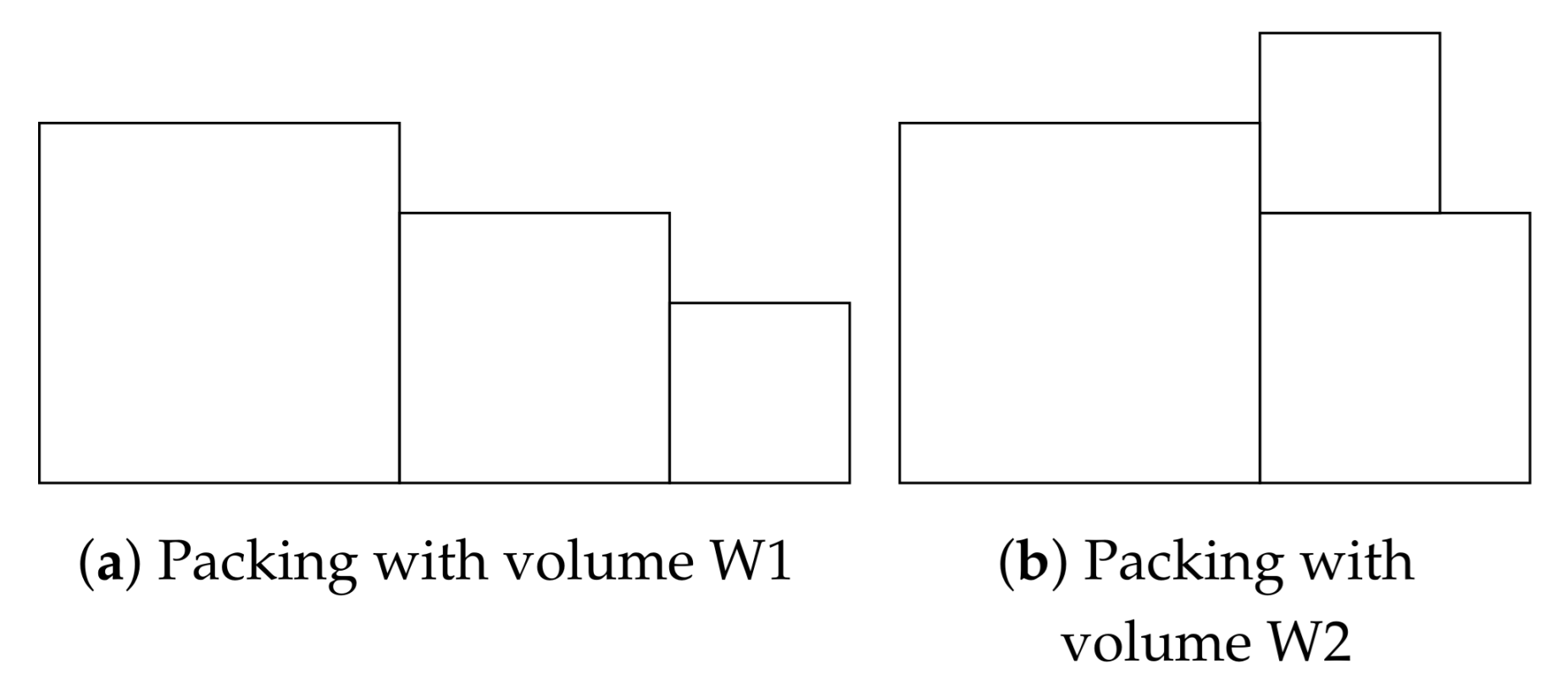
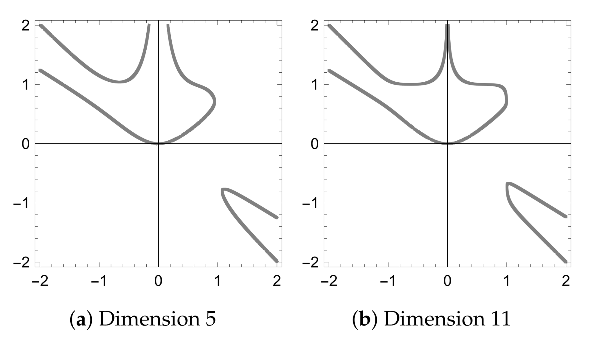
We show, that there are only two important packing configurations. Their volumes are $W_1=x^4(x+y+z)$ and $W_2=x^3(x+y)(y+z)$, see Figure 1. Firstly, we need to find $min\{W_1$, $W_2\}$ for each $\{x,y,z\}$. The maximum from $min\{W_1,W_2\}$ is the final result, we denote it $maxmin\{W_1,W_2\}$;

2.

Cubes with sides $x\doteq 0.946629932$, $y\doteq 0.690148624$, and $z\doteq 0.608279275$ have $W_1=W_2=1.802803792$. We prove that this volume is sufficient for packing any three cubes with a total volume of 1 in dimension 5;

3.

We obtain an estimation of the side size of the largest cube: $0.9445\le x\le 0.9939$;

4.

Using $1=x^5+y^5+z^5$ and $1>x\ge y\ge z>0$, we obtain constraints $x^5+y^5\le 1$ and $x^5+2y^5\ge 1$;

5.

$z={(1-x^5-y^5)}^{1/5}$. Therefore, it is sufficient to work only with x and y. M is a region of $\{x,y\}$ bounded by constraints from steps 3 and 4. We obtain a curve C from $W_1=W_2$, see Figure 2. Curve C divides the region M into continuous regions $C_1$ and $C_2$, see Figure 3;

6.

We clarify:

(a)

$W_1(X)<W_2(X)$ holds for $X\in C_1$. Therefore, $maxmin\{W_1,W_2\}=max{W}_1(X)$, $X\in C_1$;

(b)

$W_1(X)>W_2(X)$ holds for $X\in C_2$. Therefore, $maxmin\{W1,W2\}=max{W}_2(X)$, $X\in C_2$;

7.

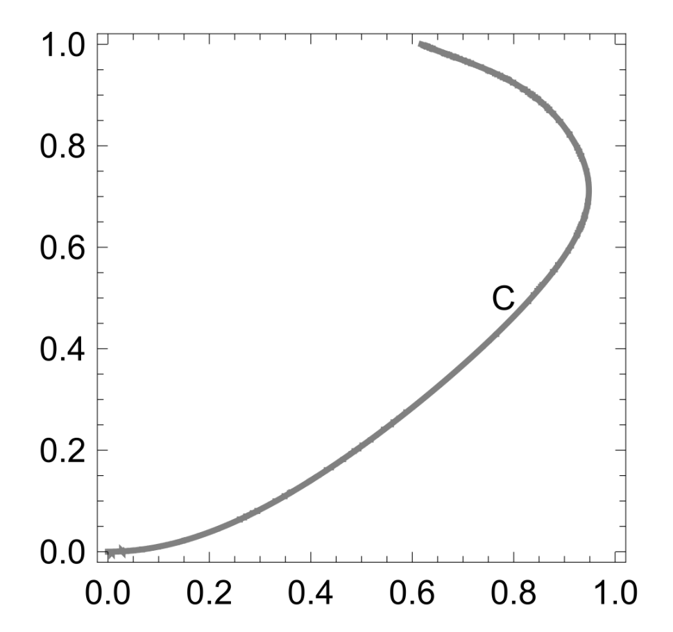
We show that the asked maximum is on curve C;

(a)

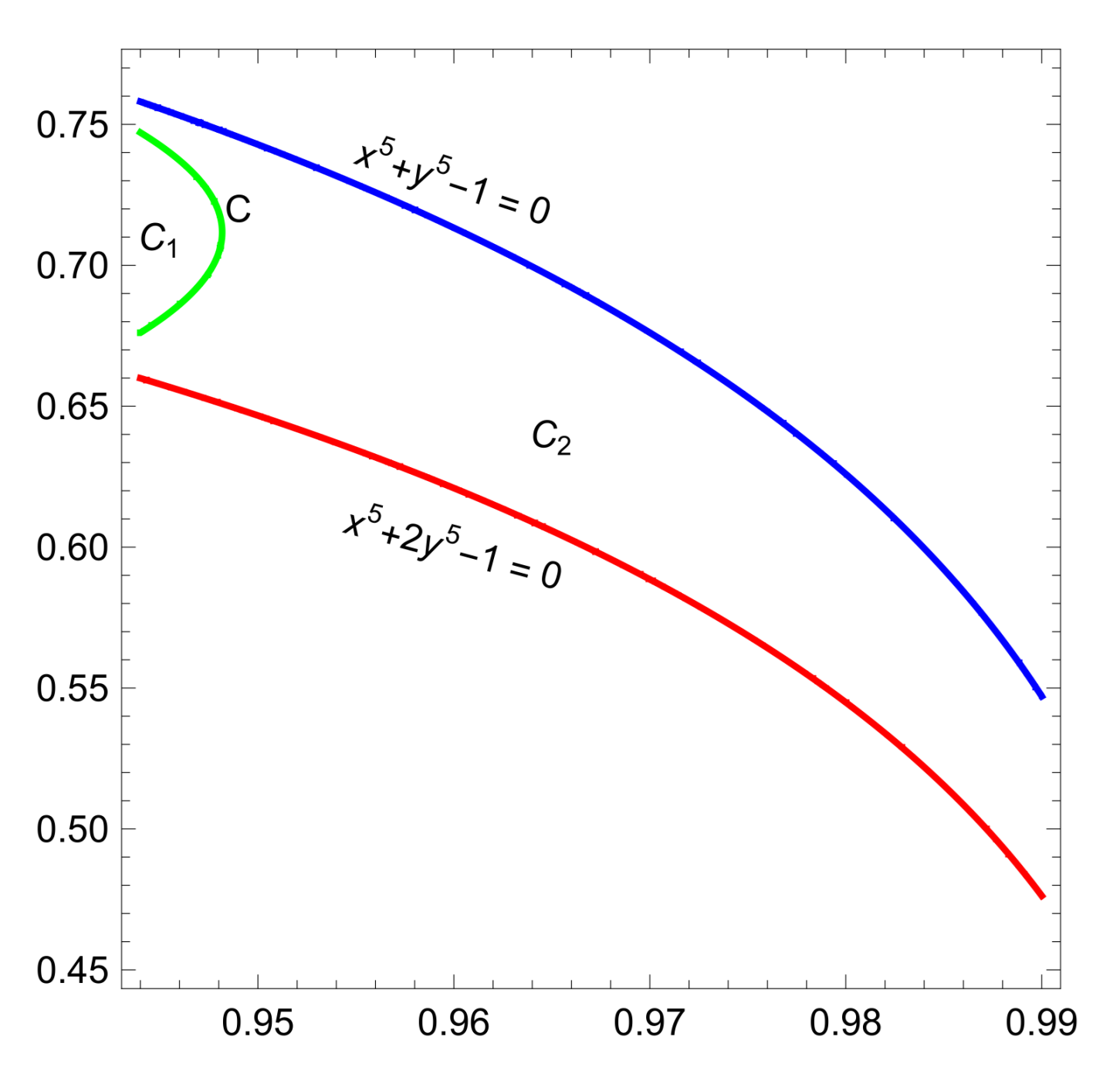
We use critical points for region $C_1$;

(b)

We were unable to use critical points on the whole $C_2$, so we gradually numerically exclude subregions. We start with comparison of maximum of subregions and 1.8 (packing with $V_3(5)>1.8$ exists).

Proof. 

Consider three cubes with edge lengths $x,y,z$ in the 5-dimensional Euclidean space, where $1>x\ge y\ge z>0$ and the total volume $x^5+y^5+z^5=1$.

We are looking for the smallest volume of a parallelepiped containing all three cubes. Therefore, from several ways of packing, we can ignore the packing that leads in any circumstances to a larger volume.

Let $X,Y,Z$ denote the cubes (sorted from the largest). We attach cubes X and Y to each other, for example, in the direction of the fifth dimension. Parallelepiped containing cubes X and Y has volume $x^4(x+y)$.

If we place the cube Z to the cube X in the direction of the fifth dimension, we receive volume $x^4(x+y+z)$. We obtain volume $x^3(x+y)(x+z)$ for other four directions.

If we place the cube Z to the cube Y in the direction of the fifth dimension, we receive again $x^4(x+y+z)$. We obtain (after appropriate shifting of the cube Y) volume $x^3(x+y)(y+z)$ for other four directions.

Because $x^3(x+y)(y+z)\le x^3(x+y)(x+z)$, we can ignore packings that lead to the volume $x^3(x+y)(x+z)$.

If we start with cubes X and Z, or Z and Y, the same results are obtained.

Therefore, it is sufficient to consider only two cases of packing three cubes, see Figure 1a,b. In the first case, the volume $W_1=x^4(x+y+z)$ is sufficient for packing, in the second case, the volume $W_2=x^3(x+y)(y+z)$ is sufficient.

We need to find $maxmin\{W_1,W_2\}$ under the conditions $x^5+y^5+z^5=1$, and $1>x\ge y\ge z>0$.

For three cubes with edge lengths $x\doteq 0.946629932,$ $y\doteq 0.690148624,$ $z\doteq 0.608279275,$ a volume $W_1=W_2\doteq 1.802803792$ is necessary. Thus, $V_3(5)\ge 1.802803792$.

If $y+z\le x$ than we can pack the cubes, as shown in Figure 1b, and volume $V_2(5)$ is sufficient, $V_2(5)\doteq 1.484663669$ for cubes with edge lengths $x\doteq 0.984432006$ and $y\doteq 0.596398035$.

Let us consider only the case that $y+z>x$. From $y^5\le z^5+y^5=1-x^5$ we find $y\le \sqrt[5]{1-x^5},$ and, therefore, $y+z\le 2y\le 2\sqrt[5]{1-x^5}$. Then, $x<y+z\le 2\sqrt[5]{1-x^5}$ and, therefore, $x^5<2^5(1-x^5)$. We attain the upper bound for $x,$ $x\le \frac{2}{\sqrt[5]{33}}$. $x\ge y\ge z$ and $x^5+y^5+z^5=1$, therefore, $x^5\ge \frac{1}{3}$ and $x\ge \frac{1}{\sqrt[5]{3}}$. This implies that we can consider only $x\in \left. [\frac{1}{\sqrt[5]{3}},\frac{2}{\sqrt[5]{33}}\right]$, i.e., $0.8027\le x\le 0.9939$.

Equality $W_1=W_2$ holds if, and only if, $x^2=y^2+yz$. In this case, $z=\frac{x^2-y^2}{y}$ and $W_1=W_2=x^5+\frac{x^6}{y}$. When we substitute $z=\frac{x^2-y^2}{y}$ into $x^5+y^5+z^5=1$ we find the curve $C:$ $x^5{y}^5+y^{10}-y^5+{(x^2-y^2)}^5=0$ (Figure 2).

The interval for x can be reduced. If we choose $x\in \left. [a,b\right]$, $0<a<b<1,$ then $1-b^5\le 1-x^5\le 1-a^5$. If $y=z,$ then $1-x^5=y^5+z^5=2y^5$ and, therefore, ${\displaystyle y=\sqrt[5]{\frac{1-x^5}{2}}}$. The function $W_1=x^4(x+y+z)$ has the greatest value if $y=z$, i.e., ${\displaystyle y=\sqrt[5]{\frac{1-x^5}{2}}}$. For $x\in \left. [a,b\right]$, we find ${\displaystyle W_1\le x^4(x+2y)\le b^4\left(b+2\sqrt[5]{\frac{1-a^5}{2}}\right)}$.

Denote ${\displaystyle W_1(a,b)=b^4\left(b+2\sqrt[5]{\frac{1-a^5}{2}}\right)}$.

The inequality $W_1(a,b)<1.8021$ is valid for the intervals: $x\in \left. [0.8027,0.9190\right]$, $x\in \left. [0.9190,0.9360\right]$, $x\in \left. [0.9360,0.9410\right]$, $x\in \left. [0.9410,0.9420\right]$, $x\in \left. [0.9420,0.9430\right]$, $x\in \left. [0.9430,0.9440\right]$, $x\in \left. [0.9440,0.9445\right]$, hence for the asked maximum holds $x\ge 0.9445$.

Therefore, we have shown that the asked $maxmin\{W_1,W_2\}$ will be attained for $x\in \left. [0.9445,0.9939\right]$.

From the assumption $0<z\le y\le x<1$ follows that $x^5+y^5\le x^5+y^5+z^5=1$ and also $1=x^5+y^5+z^5\le x^5+2y^5$.

Consider the closed region M determined by inequalities $0.9445\le x\le 0.9939,$ $x^5+y^5\le 1$, $x^5+2y^5\ge 1$. The curve C divides the region M into two open regions $C_1,C_2,$ (Figure 3).

We are looking for $\mathit{max}\mathit{min}\{W_1,W_2\},$ when $W_1=x^4(x+y+z),$ $W_2=x^3(x+y)(y+z)$. From the condition $x^5+y^5+z^5=1$ we find

$$W_1=W_1(x,y)=x^4(x+y+\sqrt[5]{1-x^5-y^5}),$$

(1)

$$W_2=W_2(x,y)=x^3(x+y)(y+\sqrt[5]{1-x^5-y^5}).$$

(2)

Let $\overline{C_i}$ denote the closure of the set $C_i$. The functions $W_1,W_2$ are continuous on M and the equality $W_1=W_2$ holds just in the points of the curve C.

Take the point $A_1=(0.945,0.70)\in C_1$. The inequality $W_1(X)<W_2(X)$ holds in every point $X\in C_1$, because of $W_1(A_1)<W_2(A_1)$. Therefore, for the asked maximum holds $\underset{X\in \overline{C_1}}{max}min\{W_1(X),W_2(X)\}=\underset{X\in \overline{C_1}}{max}\left\{W_1(X)\right\}$.

Take the point $A_2=(0.965,0.65)\in C_2$. The inequality $W_1(X)>W_2(X)$ holds in every point $X\in C_2,$ because of $W_1(A_2)>W_2(A_2)$. Therefore, for the asked maximum holds $\underset{X\in \overline{C_2}}{max}min\{W_1(X),W_2(X)\}=\underset{X\in \overline{C_2}}{max}\left\{W_2(X)\right\}$.

On the compact set $\overline{C_1}$ the function (1) has its maximum in some point B.

It holds ${\displaystyle \frac{\partial W_1}{\partial y}=x^4\left(1-\frac{y^4}{\sqrt[5]{{(1-x^5-y^5)}^4}}\right)}$. The equality ${\displaystyle \frac{\partial W_1}{\partial y}=0}$ holds if $x^5+2y^5-1=0$ but the points of the curve $x^5+2y^5-1=0$ do not belong to the region $\overline{C_1}$. For every point $X\in C_1$ holds ${\displaystyle \frac{\partial W_1}{\partial y}<0.}$ Therefore, the point B must lie on the curve C.

For every point $X=(x,y),$ $x\in \left. [a,b\right]$, $y\in \left. [c,d\right]$ the inequality $z\le \sqrt[5]{1-a^5-c^5}$ holds, and so $W_1=x^4(x+y+z)\le b^4(b+d+\sqrt[5]{1-a^5-c^5})$, $W_2=x^3(x+y)(y+z)\le b^3(b+d)(d+\sqrt[5]{1-a^5-c^5})$.

Denote

$$\begin{array}{cc}\hfill W_{11}(a,b,c,d)& =b^4(b+d+\sqrt[5]{1-a^5-c^5}),\hfill \\ \hfill W_{22}(a,b,c,d)& =b^3(b+d)(d+\sqrt[5]{1-a^5-c^5}).\hfill \end{array}$$

Examine the region $C_2$.

For $x\in \left. [0.9900,0.9939\right]$, $y\in \left. [0.43,0.60\right]$ is $W_{22}<1.8$. For $x\in \left. [0.9850,0.9900\right]$, $y\in \left. [0.47,0.60\right]$ is $W_{22}<1.8$. For $x\in \left. [0.9800,0.9850\right]$ and, step by step, for $y\in \left. [0.51,0.56\right]$, $\left. [0.56,0.60\right]$, $\left. [0.60,0.65\right]$ is always $W_{22}<1.8$.

For $x\in \left. [0.975,0.980\right]$ and, step by step, for $y\in \left. [0.54,0.60\right]$, $\left. [0.60,0.64\right]$, $\left. [0.64,0.7\right]$ is always $W_{22}<1.8$.

For $x\in \left. [0.970,0.975\right]$, and, step by step, for $y\in \left. [0.56,0.61\right]$, $\left. [0.61,0.63\right]$, $\left. [0.63,0.65\right]$, $\left. [0.65,0.68\right]$ is always $W_{22}<1.8$.

For $x\in \left. [0.965,0.970\right]$ and, step by step, for $y\in \left. [0.58,0.61\right]$, $\left. [0.61,0.63\right]$, $\left. [0.63,0.64\right]$, $\left. [0.64,0.65\right]$, $\left. [0.65,0.66\right]$, $\left. [0.66,0.67\right]$, $\left. [0.67,0.69\right]$, $\left. [0.69,0.75\right]$ is always $W_{22}<1.8$.

For $x\in \left. [0.960,0.965\right]$ and, step by step, for $y\in \left. [0.60,0.62\right]$, $\left. [0.62,0.63\right]$, $\left. [0.63,0.635\right]$, $\left. [0.635,0.64\right]$, $\left. [0.64,0.644\right]$, $\left. [0.644,0.647\right]$, $\left. [0.647,0.65\right]$, $\left. [0.65,0.652\right]$, $\left. [0.652,0.654\right]$, $\left. [0.654,0.656\right]$, $\left. [0.656,0.658\right]$, $\left. [0.658,0.66\right]$, $\left. [0.66,0.662\right]$, $\left. [0.662,0.664\right]$, $\left. [0.664,0.666\right]$, $\left. [0.666,0.668\right]$, $\left. [0.668,0.670\right]$, $\left. [0.670,0.673\right]$, $\left. [0.673,0.677\right]$, $\left. [0.677,0.680\right]$, $\left. [0.680,0.685\right]$, $\left. [0.685,0.695\right]$, $\left. [0.695,0.72\right]$ is always $W_{22}<1.8$.

For $x\in \left. [0.955,0.960\right]$ and, step by step, for $y\in \left. [0.620,0.630\right]$, $\left. [0.630,0.635\right]$, $\left. [0.635,0.638\right]$, $\left. [0.638,0.640\right]$, $\left. [0.640,0.641\right]$, $\left. [0.641,0.642\right]$, $\left. [0.697,0.698\right]$, $\left. [0.698,0.700\right]$, $\left. [0.700,0.703\right]$, $\left. [0.703,0.709\right]$, $\left. [0.709,0.724\right]$, $\left. [0.724,0.730\right]$ is always $W_{22}<1.8$.

We do not exclude the region $x\in \left. [0.9550,0.9600\right]$, $y\in \left. [0.642,0.697\right]$ in this way, it is not effective.

We have

From (2): $\frac{\partial W_2}{\partial x}=\frac{x^2}{\sqrt[5]{{(1-x^5-y^5)}^4}}\left. [(4x+3y)(y\sqrt[5]{{(1-x^5-y^5)}^4}+1-y^5)-5x^6-4x^{5}y\right]$ and $\frac{\partial W_2}{\partial y}=\frac{x^3}{\sqrt[5]{{(1-x^5-y^5)}^4}}\left. [(x+2y)\sqrt[5]{{(1-x^5-y^5)}^4}+1-x^5-2y^5-x{y}^4\right]$.

$\frac{x^2}{\sqrt[5]{{(1-x^5-y^5)}^4}}>0$ and $\frac{x^3}{\sqrt[5]{{(1-x^5-y^5)}^4}}>0$, therefore, for every point $X=(x,y),x\in \left. [a,b\right]$, $y\in \left. [c,d\right]$ we have two inequalities:

$$(4x+3y)(y\sqrt[5]{{(1-x^5-y^5)}^4}+1-y^5)-x^5(5x+4y)\le$$

$$\le (4b+3d)(d\sqrt[5]{{(1-a^5-c^5)}^4}+1-c^5)-a^5(5a+4c)$$

and

$$(x+2y)\sqrt[5]{{(1-x^5-y^5)}^4}+1-x^5-2y^5-x{y}^4\ge$$

$$\ge (a+2c)\sqrt[5]{{(1-b^5-d^5)}^4}+1-b^5-2d^5-b{d}^4$$

Denote

$$\begin{array}{cc}\hfill DW2x(a,b,c,d)& =(4b+3d)(d\sqrt[5]{{(1-a^5-c^5)}^4}+1-c^5)-a^5(5a+4c),\hfill \\ \hfill DW2y(a,b,c,d)& =(a+2c)\sqrt[5]{{(1-b^5-d^5)}^4}+1-b^5-2d^5-b{d}^4.\hfill \end{array}$$

For $x\in \left. [0.955,0.960\right]$ and $y\in \left. [0.642,0.670\right]$ is $DW2x(a,b,c,d)<0$ and, therefore, ${\displaystyle \frac{\partial W_2}{\partial x}<0}$.

For $x\in \left. [0.955,0.960\right]$ and $y\in \left. [0.670,0.697\right]$ is also $DW2x(a,b,c,d)<0$ and, therefore, ${\displaystyle \frac{\partial W_2}{\partial x}<0}$.

Therefore, the asked maximum cannot be achieved for $x\in \left. [0.955,0.960\right]$.

For $x\in \left. [0.950,0.955\right]$ and, step by step, for $y\in \left. [0.630,0.636\right]$, $\left. [0.636,0.639\right]$, $\left. [0.639,0.640\right]$, $\left. [0.640,0.641\right]$, $\left. [0.717,0.718\right]$, $\left. [0.718,0.720\right]$, $\left. [0.720,0.725\right]$, $\left. [0.725,0.738\right]$, $\left. [0.738,0.750\right]$ is always $W_{22}<1.8$.

We do not exclude the region $x\in \left. [0.950,0.955\right]$, $y\in \left. [0.641,0.717\right]$ in this way, it is not effective.

For $x\in \left. [0.950,0.955\right]$ and $y\in \left. [0.641,0.671\right]$ is $DW2y(a,b,c,d)>0$ and, therefore, ${\displaystyle \frac{\partial W_2}{\partial y}>0}$.

For $x\in \left. [0.950,0.955\right]$ and $y\in \left. [0.671,0.700\right]$ is $DW2x(a,b,c,d)<0$ and, therefore, ${\displaystyle \frac{\partial W_2}{\partial x}<0}$.

For $x\in \left. [0.950,0.955\right]$ and $y\in \left. [0.700,0.717\right]$ is $DW2x(a,b,c,d)<0$ and, therefore, ${\displaystyle \frac{\partial W_2}{\partial x}<0}$.

This implies that the asked maximum cannot be achieved for $x\in \left. [0.950,0.955\right]$.

For $x\in \left. [0.9475,0.9500\right]$ and, step by step, for $y\in \left. [0.640,0.649\right]$, $\left. [0.649,0.653\right]$, $\left. [0.653,0.655\right]$, $\left. [0.655,0.656\right]$, $\left. [0.656,0.657\right]$, $\left. [0.719,0.720\right]$, $\left. [0.720,0.722\right]$, $\left. [0.722,0.726\right]$, $\left. [0.726,0.735\right]$, $\left. [0.735,0.750\right]$ is always $W_{22}<1.8$.

We do not exclude the region $x\in \left. [0.9475,0.9500\right]$, $y\in \left. [0.657,0.719\right]$ in this way, it is not effective.

For $x\in \left. [0.9475,0.9500\right]$ and $y\in \left. [0.657,0.684\right]$ is $DW2y(a,b,c,d)>0$ and, therefore, ${\displaystyle \frac{\partial W_2}{\partial y}>0}$.

For $x\in \left. [0.9475,0.9500\right]$ and $y\in \left. [0.684,0.719\right]$ is $DW2x(a,b,c,d)<0$ and, therefore, ${\displaystyle \frac{\partial W_2}{\partial x}<0}$.

This implies that the asked maximum cannot be achieved for $x\in \left. [0.9475,0.9500\right]$, see Figure 4.

For $x\in \left. [0.9445,0.9475\right]$ and, step by step, for $y\in \left. [0.650,0.653\right]$, $\left. [0.653,0.655\right]$, $\left. [0.655,0.656\right]$, $\left. [0.656,0.657\right]$ is always $W_{22}<1.8$.

For $x\in \left. [0.9445,0.9475\right]$ and $y\in \left. [0.657,0.690\right]$ is $DW2y(a,b,c,d)>0$ and, therefore, ${\displaystyle \frac{\partial W_2}{\partial y}>0}$.

For $x\in \left. [0.9445,0.9475\right]$ and $y\in \left. [0.690,0.700\right]$ is $DW2x(a,b,c,d)<0$ and, therefore, ${\displaystyle \frac{\partial W_2}{\partial x}<0}$.

For $x\in \left. [0.9445,0.9475\right]$ and, step by step, for $y\in \left. [0.720,0.726\right]$, $\left. [0.726,0.743\right]$, $\left. [0.743,0.760\right]$ is always $W_{11}<1.8$.

So function (2) on the compact set $\overline{C_2}$ must achieve its maximum in some point of the curve C. It is the same point B as above.

We ask constrained maximum of the function

$${\displaystyle W(x,y)=x^5+\frac{x^6}{y}}$$

(3)

on the curve C

$$C(x,y)=x^5{y}^5+y^{10}-y^5+{(x^2-y^2)}^5=0$$

(4)

for $x\in \left. [0.9445,0.9475\right]$.

System of equations ${\displaystyle \frac{\partial W}{\partial x}\frac{\partial C}{\partial y}-\frac{\partial W}{\partial y}\frac{\partial C}{\partial x}=0}$ and $C(x,y)=0$ has the form

$$7x^6{y}^5+12x{y}^{10}-6x{y}^5+5x^5{y}^6+10y^{11}-5y^6+{(x^2-y^2)}^4(2x^3-10y^3-12x{y}^2)=0,$$

$$x^5{y}^5+y^{10}-y^5+{(x^2-y^2)}^5=0.$$

The solution is $x\doteq 0.946629932,y\doteq 0.690148624,$ and then $z\doteq 0.608279275$. □

If we generalize considerations from the proof, we will achieve the curve $C:x^d{y}^d+y^{2d}-y^d+{(x^2-y^2)}^d=0$, where d is dimension. The graph of the curve C depends on the parity of d, see Figure 5 and Figure 6. Considering only the values $1>x\ge y>0$, the shape of the curve C is similar, regardless of parity, see Figure 2.

For $d\le 10$ the asked maximum is achieved on the curve C. For dimensions 7, 9 and 10 the resultsare:

$$\begin{array}{cc}\hfill V_3(7)& \doteq 2.05909680\mathrm{and}x\doteq 0.978852925,y\doteq 0.703495386,z\doteq 0.658493716,\hfill \\ \hfill V_3(9)& \doteq 2.21897778\mathrm{and}x\doteq 0.991008397,y\doteq 0.704394561,z\doteq 0.689849087,\hfill \\ \hfill V_3(10)& \doteq 2.27220126\mathrm{and}x\doteq 0.993961280,y\doteq 0.702901846,z\doteq 0.702641521.\hfill \end{array}$$

Let P is intersection the constraint curve $x^d+2y^d-1=0$ and the curve C. If $d=11$, then the constrained extreme on the curve C does not meet the required assumption $y\ge z$. Therefore, the asked maximum must be on the constraint curve to the left of point P or on the curve C above P, see Figure 7. The same situation occurs for $d=12$ and $d=13$.

$V_3(11)\doteq 2.31533581$ and $x\doteq 0.994989464$, $y=z\doteq 0.719809616$.

$V_3(12)\doteq 2.35315527$ and $x\doteq 0.995762712$, $y=z\doteq 0.734956999$,

$V_3(13)\doteq 2.38661963$ and $x\doteq 0.996369617$, $y=z\doteq 0.748358875$.

3. Conclusions

The issue of packing squares is an old problem and even though there are multiple partial results, it remains unresolved. We investigated a modified problem: packing three cubes in 5-dimensional space. We also calculated results for dimensions $7,9,10,11,12,13$.

Considering the previous results by [17,18,19], we can say that solution is located on the curve C for dimensions $4\dots 10$. It means, that there are two (different) packings that give (the same) the largest volume.

There seems to be only a single maximal packing for dimensions greater than 10. In this packing, two smallest cubes are the same. However, the paper confirms it only for dimensions 11, 12, 13.

There is a space for several improvements in our work: Is it possible to find a $V_3(d)$ without long numerical calculations? Is it true that two different maximum packings exist only for dimensions less than 11?

References

- Moser, L. Poorly Formulated Unsolved Problems of Combinatorial Geometry, Mimeographed List. 1966. Available online: https://www.google.com/url?sa=t&rct=j&q=&esrc=s&source=web&cd=&ved=2ahUKEwjNi_6E2MvyAhVQ82EKHXwkDswQFnoECAgQAQ&url=https%3A%2F%2Farxiv.org%2Fpdf%2F2104.09324&usg=AOvVaw04NiNvduVgpLb0NhXT63Zw (accessed on 8 July 2021).
- Brass, P.; Moser, W.O.J.; Pach, J. Research Problems in Discrete Geometry; Springer: New York, NY, USA, 2005. [Google Scholar]
- Croft, H.T.; Falconer, K.J.; Guy, R.K. Unsolved Problems in Geometry; Springer: New York, NY, USA, 1991. [Google Scholar]
- Moon, J.W.; Moser, L. Some packing and covering theorems. Colloq. Math. 1967, 17, 103–110. [Google Scholar] [CrossRef]
- Moser, W. Problems, problems, problems. Discret. Appl. Math. 1991, 31, 201–225. [Google Scholar] [CrossRef][Green Version]
- Moser, W.; Pach, J. Research Problems in Discrete Geometry; McGill University: Montreal, QC, Canada, 1994. [Google Scholar]
- Kleitman, D.J.; Krieger, M.M. An optimal bound for two dimensional bin packing. In Proceedings of the 16th Annual Symposium on Foundations of Computer Science, Berkeley, CA, USA, 13–15 October 1975; pp. 163–168. [Google Scholar]
- Novotný, P. A note on a packing of squares. Stud. Univ. Transp. Commun. Žilina Math.-Phys. Ser. 1995, 10, 35–39. [Google Scholar]
- Novotný, P. On packing of four and five squares into a rectangle. Note Mat. 1999, 19, 199–206. [Google Scholar]
- Novotný, P. Využitie počítača pri riešení ukladacieho problému. In Proceedings of the Symposium on Computational Geometry, Kočovce, Slovak Republic, 9–11 October 2002; pp. 60–62. (In Slovak). [Google Scholar]
- Novotný, P. On packing of squares into a rectangle. Arch. Math. 1996, 32, 75–83. [Google Scholar]
- Hougardy, S. On packing squares into a rectangle. Comput. Geom. 2011, 44, 456–463. [Google Scholar] [CrossRef]
- Meir, A.; Moser, L. On packing of squares and cubes. J. Comb. Theory 1968, 5, 126–134. [Google Scholar] [CrossRef][Green Version]
- Novotný, P. Ukladanie kociek do kvádra. In Proceedings of the Symposium on Computational Geometry, Kočovce, Slovak Republic, 19–21 October 2011; pp. 100–103. (In Slovak). [Google Scholar]
- Novotný, P. Pakovanie troch kociek. In Proceedings of the Symposium on Computational Geometry, Kočovce, Slovak Republic, 27–29 September 2006; pp. 117–119. (In Slovak). [Google Scholar]
- Novotný, P. Najhoršie pakovateľné štyri kocky. In Proceedings of the Symposium on Computational Geometry, Kočovce, Slovak Republic, 24–26 October 2007; pp. 78–81. (In Slovak). [Google Scholar]
- Bálint, V.; Adamko, P. Minimalizácia objemu kvádra pre uloženie troch kociek v dimenzii 4. Slov. Pre Geom. Graf. 2015, 12, 5–16. (In Slovak) [Google Scholar]
- Bálint, V.; Adamko, P. Minimization of the parallelepiped for packing of three cubes in dimension 6. In Proceedings of the Aplimat: 15th Conference on Applied Mathematics, Bratislava, Slovak Republic, 2–4 February 2016; pp. 44–55. [Google Scholar]
- Sedliačková, Z. Packing Three Cubes in 8-Dimensional Space. J. Geom. Graph. 2018, 22, 217–223. [Google Scholar]
- Adamko, P.; Bálint, V. Universal asymptotical results on packing of cubes. Stud. Univ. Žilina Math. Ser. 2016, 28, 1–4. [Google Scholar]
Publisher’s Note: MDPI stays neutral with regard to jurisdictional claims in published maps and institutional affiliations. |
© 2021 by the authors. Licensee MDPI, Basel, Switzerland. This article is an open access article distributed under the terms and conditions of the Creative Commons Attribution (CC BY) license (https://creativecommons.org/licenses/by/4.0/).
Share and Cite
Sedliačková, Z.; Adamko, P. Packing Three Cubes in D-Dimensional Space. Mathematics 2021, 9, 2046. https://doi.org/10.3390/math9172046
Sedliačková Z, Adamko P. Packing Three Cubes in D-Dimensional Space. Mathematics. 2021; 9(17):2046. https://doi.org/10.3390/math9172046
Chicago/Turabian StyleSedliačková, Zuzana, and Peter Adamko. 2021. "Packing Three Cubes in D-Dimensional Space" Mathematics 9, no. 17: 2046. https://doi.org/10.3390/math9172046
APA StyleSedliačková, Z., & Adamko, P. (2021). Packing Three Cubes in D-Dimensional Space. Mathematics, 9(17), 2046. https://doi.org/10.3390/math9172046