Article

Generalization Second Order Macroscopic Traffic Models via Relative Velocity of the Congestion Propagation

by
Yaroslav Kholodov
1,*,
Andrey Alekseenko
2,
Viktor Kazorin
3 and
Alexander Kurzhanskiy
4
1
Division of Applied Mathematics, Moscow Institute of Physics and Technology, Innopolis University, 420500 Innopolis, Russia
2
Institute for Computer Aided Design of RAS, 123056 Moscow, Russia
3
Lab of Data Analysis and Bioinformatics, Innopolis University, 420500 Innopolis, Russia
4
California Partners for Advanced Transportation Technology, University of California, Berkeley, CA 94720, USA
*
Author to whom correspondence should be addressed.
Mathematics 2021, 9(16), 2001; https://doi.org/10.3390/math9162001
Submission received: 17 June 2021 / Revised: 27 July 2021 / Accepted: 18 August 2021 / Published: 21 August 2021

Abstract

:
This paper presents a generalized second-order hydrodynamic traffic model. Its central piece is the expression for the relative velocity of the congestion (compression wave) propagation. We show that the well-known second-order models of Payne–Whitham, Aw–Rascal and Zhang are all special cases of the featured generalized model, and their properties are fully defined by how the relative velocity of the congestion is expressed. The proposed model is verified with traffic data from a segment of the Interstate 580 freeway in California, USA, collected by the California DOT’s Performance Measurement System (PeMS).

1. Introduction

In this paper, we introduce a new second-order hydrodynamic traffic model that generalizes the existing second-order models. The key feature of the new model is the notion of the relative velocity of the congestion (compression wave) propagation. This quantity can be obtained empirically from traffic detector measurements. Moreover, knowledge of the congestion relative velocity obviates the need for the fundamental diagram. We test the proposed model through numerical experiments using typical traffic detector data from the Performance Measurement System (PeMS) ([1]), on the I-580 freeway in California, USA.
An extensive development of gas dynamics (generalized conservation laws, stable differencing schemes) occurred in the 1950s, when the first macroscopic (hydrodynamic) models were developed. In those models, traffic flow was likened to a flow of “motivated” compressible liquid. For instance, the Lighthill–Whitham–Richards (LWR) model ([2,3]) describes the traffic flow through the law of conservation of vehicles. This model postulates the unique dependence of traffic flow on traffic density, which is called a fundamental diagram, and assumes a unique relationship between traffic speed v ( t , x ) and density ρ ( t , x ) : v ( t , x ) = V ( ρ ( t , x ) ) . Here, ρ ( t , x ) denotes vehicle density—the number of vehicles per unit length of the road at time t around the position x; and v ( t , x ) denotes mean traffic speed at time t around the position x. The function V ( ρ ) is non-increasing: V ρ 0 . We denote the flow (i.e., the number of vehicles passing a reference point in unit time) as Q ( ρ ) = ρ V ( ρ ) . The function is referred to as the fundamental diagram (although sometimes this name is reserved for V ( ρ ) ). The vehicle conservation law in the LWR model is expressed in the differential form of a continuity equation with zero right-hand side:
ρ t + ( ρ v ) x = ρ t + ρ V ( ρ ) x = ρ t + Q ( ρ ) x = 0 v ( t , x ) = V ( ρ ( t , x ) )
Later, the class of macroscopic models has expanded to systems of non-linear hyperbolic second-order PDEs, where the unique dependence of traffic density and speed is no longer assumed ([4,5,6,7,8,9,10,11,12]). These models differ in the way that they describe the dependency of traffic flow (or velocity) on density. Here, we will discuss some popular second-order models and show how they can be generalized using the relative velocity of the congestion.
We start with the Payne–Whitham model ([4,13]) with zero right-hand side to simplify the subsequent calculations:
ρ t + Q x = 0 v t + V v x + c 0 2 ρ ρ x = 0
where c 0 < 0 is the so-called traffic ‘sound speed’, and generalize it for the arbitrary form of the relative velocity of the congestion, c ( ρ ) :
c ( ρ ) 2 = P ( ρ ) ρ P ( ρ ) = 0 ρ c ( ρ ˜ ) 2 d ρ ˜
With P ( ρ ) defined in (3), model (2) can be rewritten ([8]):
ρ t + Q x = ρ t + Q ρ ρ x = ρ t + v ρ x + ρ v x = 0 v t + v v x + c ( ρ ) 2 ρ ρ x = v t + v v x + 1 ρ P ρ ρ x = v t + v v x + 1 ρ P x = 0
which generalizes (2). The proposed model (4) can also be written in the conservative form:
ρ t + ( ρ v ) x = 0 ( ρ v ) t + ρ v 2 + P ( ρ ) ) x = 0
The work ([8]) also proposed the model (4) in anisotropic form, defined by system:
ρ t + Q x = ρ t + v ρ x + ρ v x = 0 v t + v v x + c ( ρ ) v x = v t + v + ρ V ( ρ ) ρ v x = 0
where the relative velocity of the congestion propagation is expressed through the derivative of the equilibrium speed: c ( ρ ) = ρ V ( ρ ) ρ
Note that system (6) is almost identical to the system proposed in ([7]) when its second equation is in a non-conservative form. The difference is in the form of c ( ρ ) . In ([7]), the smooth function P ( ρ ) is used instead of the equilibrium speed V ( ρ ) :
ρ t + Q x = ρ t + v ρ x + ρ v x = 0 v t + v ρ P ( ρ ) ρ v x = v t + v + ρ V ( ρ ) ρ v x = 0
From the physical standpoint, the use of the equilibrium speed V ( ρ ) in (7) instead of an arbitrary smooth increasing function P ( ρ ) ρ γ , γ > 0 is more justified (see ([8])), as the function V ( ρ ) is generally not smooth in points of transition between different traffic phases.
A system similar to (6), but with an additional relaxation term β ( ρ , v ) ( V ( ρ ) v ) in the right-hand side, was introduced in ([10,11]):
ρ t + Q x = ρ t + v ρ x + ρ v x = 0 v t + v + ρ V ( ρ ) ρ v x = β ( ρ , v ) ( V ( ρ ) v )
where the equilibrium speed is expressed as V ( ρ ) = V m a x 1 ρ ρ m a x n 1 n 2 in ([10,11]); and as V ( ρ ) = V m a x 1 exp λ V m a x 1 ρ 1 ρ m a x in ([11]).
The rest of the paper is organized as follows. Section 2 has two parts: in Section 2.1 the relative velocity of congestion propagation is expressed using the model variables, traffic velocity v and density ρ ; Section 2.2 proposes the generalized second-order model and shows, using the relative velocity of the congestion (compression wave) propagation, that the existing second-order models are special cases of the proposed one. Section 3 presents the discretized numerical method for model simulation. Section 4 discusses the simulation results, which support the proposition that different second-order models with the same expression for the relative velocity of the congestion behave similarly. Section 5 concludes the paper.

2. Generalized Model

2.1. Relative Velocity of the Congestion Propagation

First, we need to find a formal way to express the relative velocity of the congestion propagation, c ( ρ ) , or traffic pressure P ( ρ ) = 0 ρ c ( ρ ˜ ) 2 d ρ ˜ using the model variables, traffic speed v and density ρ .
From the continuity equation, we know that:
ρ t + Q x = ρ t + Q ρ ρ x = 0 1 ρ x = Q ρ ρ t
Using this, we express partial derivative P ρ = P ρ via P x = P x :
P ρ = P ρ = P x x ρ = P x ρ x = Q ρ ρ t P x
Then, we express P x = P x from the second equation of (5):
( ρ v ) t + ρ v 2 + P ( ρ ) x = Q t + Q v x + P x = 0
P x = P x = Q t + Q v x = Q t + Q v Q Q x = ρ t = Q x = Q t Q v Q ρ t
and substitute P x into the Equation (9):
P ρ = Q p ρ t P x = Q p ρ t Q t Q v Q ρ t = Q ρ Q ρ Q v Q = Q ρ 2 Q v ρ
Taking Q ρ 2 and Q v ρ from the known relations:
Q ρ 2 = ( ρ v ) ρ 2 = v + ρ v ρ 2 = v 2 + 2 ρ v v ρ + ρ 2 v ρ 2
( Q v ) ρ = ( ρ v 2 ) ρ = v 2 + ρ v 2 ρ = v 2 + 2 ρ v v ρ
and using them in the expression of P ρ = P ρ , we obtain the equation for c ( ρ ) 2 :
c ( ρ ) 2 = P ( ρ ) ρ = Q ρ 2 Q v ρ = ρ 2 v ρ 2
The sign: c ( ρ ) = ± P ( ρ ) ρ remains to be determined. For that, we substitute expression for c ( ρ ) 2 in the second equation of (4):
v t + v v x + c ( ρ ) 2 ρ ρ x = v t + v v x + ρ v ρ v ρ ρ x = v t + v + ρ v ρ = v t + v + c ( ρ ) v x = 0
and finally obtain the formula for the relative velocity of the congestion propagation:
c ( ρ ) = ρ v ρ

2.2. Model Equations

The vehicle conservation law in the LWR model (1) is expressed by the continuity equation in the differential form with zero right-hand side. Accounting for variations in vehicle numbers, for example, due to lane changes or freeway entrances and exits, Equation (1) takes the form:
ρ t + Q x = ρ t + ρ v x + v ρ x = f 0
where f 0 is the number of vehicles entering (positive) or leaving (negative) in unit time. Equation (13) by itself is not sufficient for an adequate description of all the traffic flow phases ([5]). To correct this, we use the differential transformation of the conservation law ([14]). We multiply (13) by v ρ :
v ρ ρ t + Q x = v ρ ρ t + v ρ ρ v x + v ρ x = v ρ f 0
and get:
v t + v v x + ρ v ρ v x = v t + v + ρ v ρ v x = v ρ f 0
Recall that c ( ρ ) = ρ v ρ is the relative velocity of the congestion propagation. Now, we can rewrite Equations (13) and (14) in their final form:
ρ t + Q x = ρ t + ρ v x + v ρ x = f 0 v t + v + ρ v ρ v x = v t + v + c ( ρ ) v x = v ρ f 0
Thus, we constructed a second-order macroscopic model that does not assume a unique dependency between traffic speed and density, as in the LWR. The right-hand side f 0 of the first equation of (15) accounts for the number of vehicles incoming (positive) or leaving (negative) in unit time. Looking at the right-hand side of the velocity equation in (15), we see the impact of these vehicles on traffic speed.
The number of left and right boundary conditions in (15) depends on the signs of the eigenvalues of the system: λ 1 = v , λ 2 = v + ρ v ρ . Since λ 1 = v is always 0 , we need to know the sign of λ 2 = v + ρ v ρ . At a freeway entrance, there are two boundary conditions, if λ 1 > 0 , λ 2 > 0 ; one, if λ 1 > 0 , λ 2 0 ; or zero, if λ 1 = 0 , λ 2 0 . The opposite is true for a freeway exit: zero boundary conditions, if both λ 1 , λ 2 0 ; one, if λ 1 0 , λ 2 < 0 . Therefore, we can use time-dependent traffic flow Q ( t ) and speed v ( t ) as boundary conditions. Besides the boundary conditions, we set the following initial conditions:
ρ ( x , 0 ) = ρ 0 ( x ) , v ( x , 0 ) = v 0 ( x )
Several shortcomings of the Payne–Whitham model (2) were pinpointed in ([5]). In particular, it was mentioned that, with strong spatial disturbances in initial conditions, negative values of velocity and/or density might appear in the solution. According to the model, the traffic is influenced by the vehicles traveling behind it, which was not possible in the case of a one-lane road. These inconsistencies arise because, initially, the system (2) (or (4)) was used to model barotropic gas that is isotropic, and all directions of motion for barotropic gas are equally probable.
Mathematically, this relates to the fact that the relative velocity of the congestion propagation, c ( ρ ) = P ( ρ ) ρ = ρ v ρ , is squared in the second equations of systems (4) and (5). Thus, these equations are not sensitive to the sign of the relative velocity and are agnostic of the congestion direction.
To resolve this issue, in system (11), we turned from c ( ρ ) 2 to c ( ρ ) and obtained the resulting second-order macroscopic model (15) with zero right-hand side. It should also be noted that once we found the expression for the relative velocity of the congestion, c ( ρ ) = ρ v ρ , the eigenvalues of the isotropic system (4), λ 1 , 2 = v ± c ( ρ ) , are transformed to λ 1 = v , λ 2 = v + c ( ρ ) v , in the system (15).
These results are stated in the following theorem.
Theorem 1.
Any macroscopic second-order hyperbolic model for the description of traffic flow dynamics can be formulated as
ρ t + v ρ x + ρ v x = f 0 v t + v + c ( ρ ) v x = v ρ f 0 + f 1
by choosing a specific form of the relative velocity of the congestion propagation, c ( ρ ) . The term f 0 in the right-hand side of the model accounts for the number of vehicles incoming or leaving in unit time. The term f 1 plays the role of a relaxation term when necessary.
Remark 1.
Note that ([8]) was the first to propose an expression for the relative velocity of the congestion propagation in the form: c ( ρ ) = ρ V ( ρ ) ρ . This differs from (12) in that, instead of the observed traffic flow velocity, it uses the equilibrium velocity V ( ρ ) . Additionally, the expression for the relative velocity of the congestion propagation, c ( ρ ) = ρ V ( ρ ) ρ , in ([8]), was derived from the car-following model ([15]), while we obtained our expression c ( ρ ) = ρ v ρ from the system (5), with no additional restrictions on values of traffic speed.
The approach of ([8]) is justified, since we need to calculate the relative velocity of the congestion for each road segment and we have only two ways of doing this:
  • First, we can define the relative velocity of the congestion propagation by using equilibrium velocity, as was carried out in ([8]), c ( ρ ) = ρ V ( ρ ) ρ . The function for equilibrium velocity V ( ρ ) (fundamental diagram) can be empirically set using traffic detector data for a long period of time for each segment of the road.
  • Second, we can do this without using equilibrium velocity or any form of a fundamental diagram. We approximate the value of the relative velocity of the congestion propagation using traffic density and velocity measured at the current time instant:
    c ( ρ ) = ρ i n + ρ o u t 2 v o u t v i n ρ o u t ρ i n
In (16), ρ i n , v i n and ρ o u t , v o u t denote the measured values of traffic densities and velocities at the current time instant at the entrance and exit of the chosen road segment. If ρ i n = ρ o u t , we can use the value of the relative velocity of congestion propagation at the previous time instant to avoid the division by zero.
As an example of our theorem application, we show how the model equations in the conservative form, proposed in ([7]),
ρ t + ( ρ v ) x = 0 ρ ( v + P ( ρ ) ) t + ρ v ( v + P ( ρ ) ) x = 0
can be derived from the system (5), using the expression for the relative velocity of the congestion in the form: c ( ρ ) = ρ P ( ρ ) ρ . The density conservation equations in both systems are identical, so we will focus on the momentum equations:
( ρ v ) t + ρ v 2 + P ( ρ ) ) x = ( ρ v ) t + ρ v 2 x + P ( ρ ) ρ ρ x = 0
( ρ v ) t + ρ v 2 x + c 2 ( ρ ) ρ x = 0
( ρ v ) t + ρ v 2 x + ρ 2 P ( ρ ) ρ 2 ρ x = 0
( ρ v ) t + ρ v 2 x + ρ 2 P ( ρ ) ρ P ( ρ ) x = 0
From the first equation of (5), using c ( ρ ) = ρ v ρ = ρ P ( ρ ) ρ , we obtain:
ρ t + Q x = ρ t + v ρ x + ρ v x = ρ t + v ρ x + ρ v ρ ρ x = 0
ρ t + v ρ P ( ρ ) ρ ρ x = 0
P ( ρ ) ρ ρ t + v ρ x ρ P ( ρ ) x = 0
P ( ρ ) t + v P ( ρ ) x ρ P ( ρ ) ρ P ( ρ ) x = 0
ρ 2 P ( ρ ) ρ P ( ρ ) x = ρ P ( ρ ) t + v P ( ρ ) x
By substituting ρ 2 P ( ρ ) ρ P ( ρ ) x = ρ P ( ρ ) t + v P ( ρ ) x into the last of (18), we get:
( ρ v ) t + ρ v 2 x + ρ P ( ρ ) t + v P ( ρ ) x = 0
( ρ v ) t + ρ v 2 x + ρ P ( ρ ) t + v P ( ρ ) x + P ( ρ ) ρ t + ( ρ v ) x = 0
( ρ v ) t + ρ P ( ρ ) t + ρ v 2 x + ρ v P ( ρ ) x = 0
ρ v + P ( ρ ) t + ρ v v + P ( ρ ) x = 0
Therefore, we arrive at the momentum equation of (17), QED.
Reversing this logic, we can easily obtain system (5) from the system (17) using the same expression for the relative velocity of the congestion, c ( ρ ) = ρ v ρ = ρ P ( ρ ) ρ .
Thus, we see that the existing second-order hydrodynamic traffic models can be generalized using the relative velocity of the congestion propagation.
Additionally, it is important to know why the transition from macroscopic first-order models to second-order models is useful: adding the momentum equation into the system obviates the need for a fundamental diagram. Instead, the relative velocity of the congestion propagation can be obtained from traffic detector measurements. This enables the model to instantly adjust to real-time road conditions.

3. Computational Method

The second-order model (15) is of a hyperbolic type. A variety of finite-difference methods for solving such systems exist. By introducing vectors W = ρ , v T and f = f 0 , v ρ f 0 + f 1 T , the system (15) can be written in the vector form:
W t + A W x = W t + Ω 1 Λ Ω W x = f
with the Jacobian:
A = v ρ 0 v + ρ v ρ = v ρ 0 v + c ρ = Ω 1 Λ Ω
In (22), Λ = λ 1 0 0 λ 2 is a diagonal matrix of eigenvalues of the Jacobian A; Ω = ω 1 ω 2 is the matrix of left eigenvectors of A; and Ω 1 is the inverse of Ω .
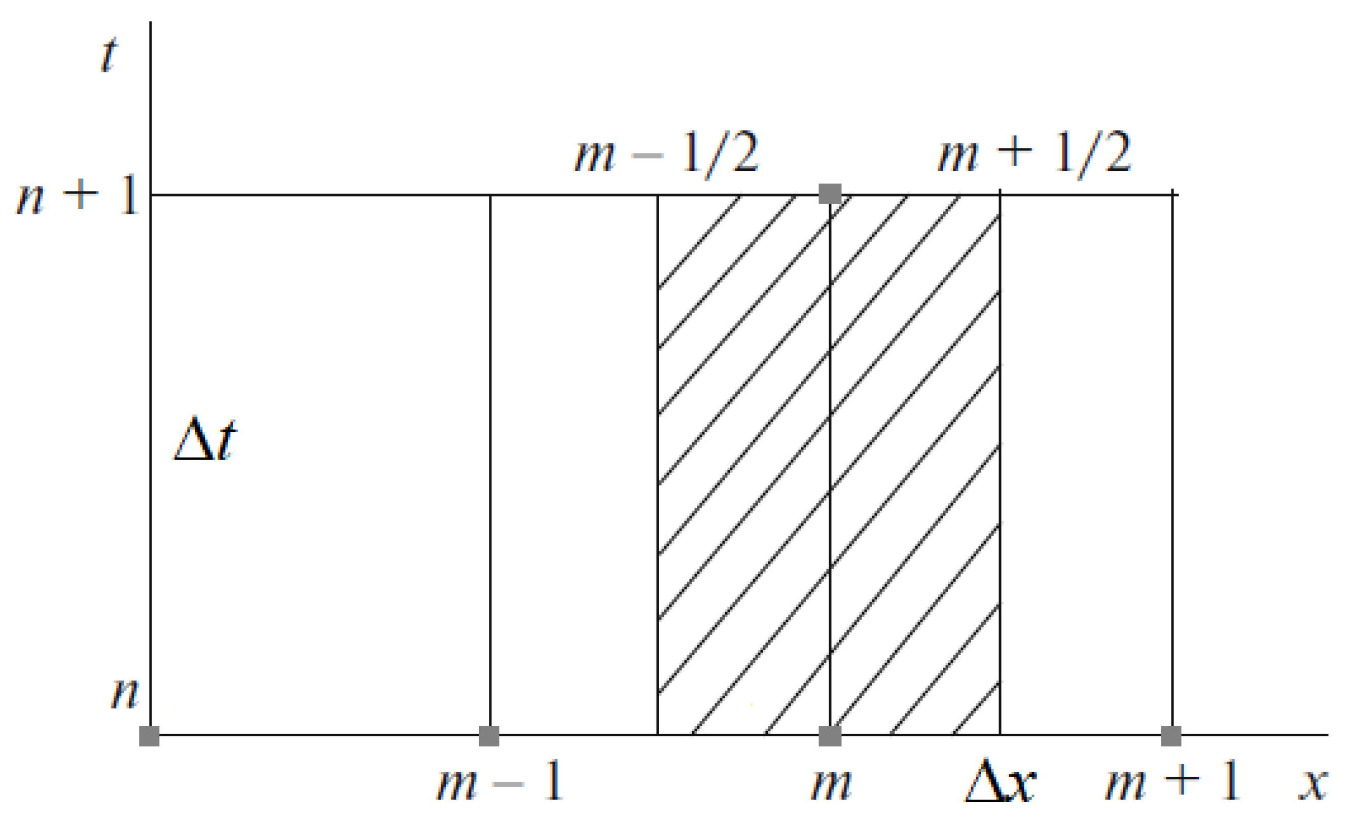
Next, we write a finite-difference approximation on the grid shown in Figure 1 by making the values of the equation variables constant at the edges of the grid:
W m n + 1 W m n Δ t + A W m + 1 2 n + 1 2 W m 1 2 n + 1 2 Δ x = W m n + 1 W m n Δ t + A W m + 1 2 n + 1 2 A W m 1 2 n + 1 2 Δ x = f m n
Here, m = 1 , , M is the grid node index along the x-axis, n = 1 , , N , is the grid node index along the t-axis, Δ t and Δ x are numerical integration steps bounded via the Courant condition: Δ t · max m | ( λ 1 , 2 ) m n | < Δ x .
For system (15), the whole family of difference schemes can be expressed as follows (Kholodov and Tsybulin, 2018):
W m n + 1 = W m n Δ t Δ x G m + 1 2 n + 1 2 G m 1 2 n + 1 2 + f m n .
The choice of the approximation method for G m ± 1 2 n + 1 2 = A W m ± 1 2 n + 1 2 in (23) is crucial for obtaining the scheme with the desired properties. When choosing a difference scheme, we presume that the solution for the model equations at every road segment is defined by the change in computed values in its boundary points. In this case, we can choose the conservative monotonic characteristic method of the first-order approximation ([16]) with the following expressions for G m ± 1 2 n + 1 2 :
G m ± 1 2 n + 1 2 = 1 2 A m ± 1 2 n W m n + W m ± 1 n ± 1 2 Ω 1 Λ Ω m ± 1 2 n W m n W m ± 1 n
These could also be more complex expressions, which allow for the building of higher-order (hence, higher-accuracy) difference schemes for a given stencil. Variable values in the neighboring nodes m ± 1 2 in (24) can be computed using a simple linear interpolation without loss of accuracy.
A m ± 1 2 n = v m n + v m ± 1 n 2 ρ m n + ρ m ± 1 n 2 0 v m n + v m ± 1 n 2 + c ρ m n + ρ m ± 1 n 2 ,
Λ m ± 1 2 n = λ 1 , m ± 1 2 n 0 0 λ 2 , m ± 1 2 n = v m n + v m ± 1 n 2 0 0 v m n + v m ± 1 n 2 + c ρ m n + ρ m ± 1 n 2 ,
Ω m ± 1 2 n = ω 1 , m ± 1 / 2 n ω 2 , m ± 1 / 2 n = 2 ρ m n + ρ m ± 1 n c ρ m n + ρ m ± 1 n 2 1 0 1 ,
Ω 1 m ± 1 2 n = ρ m n + ρ m ± 1 n 2 c ρ m n + ρ m ± 1 n 2 ρ m n + ρ m ± 1 n 2 c ρ m n + ρ m ± 1 n 2 0 1 .
To obtain the characteristic form of compatibility equations, equivalent to the system (21) along the characteristics λ 1 , 2 = d x d t , we multiply the system (21) from the left by the eigenvector matrix Ω (i.e., we compose 2 linearly independent combinations of the original equations) and bring it to the characteristic form:
Ω W t + Ω 1 Λ Ω W x = Ω W t + Λ Ω W x = Ω f .
Then, in the scalar form, this yields:
ω i · W t + λ i ω i · W x = ω i · W t + λ i W x = ω i · f , i = 1 , 2
Each of the two equations (26) is an ordinary differential equation along the characteristic λ 1 , 2 = d x d t .
We usually need to numerically integrate the compatibility conditions (26) at boundary points along the characteristics entering the integration area. For example, at the beginning of the freeway segment at boundary point t n + 1 , x 1 with negative eigenvalue λ 2 3 2 n = v 1 n + v 2 n 2 + c ρ 1 n + ρ 2 n 2 < 0 , we use:
ω 2 3 2 n · W 1 n + 1 W 1 n Δ t + λ 2 3 / 2 n W 2 n W 1 n Δ x = ω 2 3 2 n · f 1 n v 1 n + 1 = v t n + 1 , x 1
together with the boundary condition for traffic velocity v t , x 1 .
At the end of the freeway segment, we do the same for the positive λ 2 M 1 2 n = v M n + v M 1 n 2 + c ρ M n + ρ M 1 n 2 > 0 :
ω 1 , 2 M 1 2 n · W M n + 1 W M n Δ t + λ 1 , 2 M 1 2 n W M n W M 1 n x = ω 1 , 2 M 1 2 n · f 1 n ,
for both compatibility equations, because λ 1 m ± 1 2 n = v m n + v m ± 1 n 2 > 0 is always positive.
We should reiterate that the relative velocity of the congestion, c ( ρ ) in (22)–(28) can be defined using equilibrium velocity c ρ = ρ V ρ ρ as was done in ([8]). The function for equilibrium velocity V ( ρ ) (fundamental diagram) can be empirically set using historic traffic detector data for each road segment. We propose the new approach without using equilibrium velocity or any form of a fundamental diagram Q ( ρ ) . We approximate the value of the relative velocity of the congestion propagation, c ρ = ρ v ρ , using traffic density and velocity observed by traffic detection at the current time instant:
c ρ m ± 1 2 n = ρ v ρ m ± 1 2 n = ρ m n + ρ m ± 1 n 2 v m n v m ± 1 n ρ m n ρ m ± 1 n .
This approach enables our model (15) to instantly adjust to the changing road situation at runtime.

4. Numerical Results

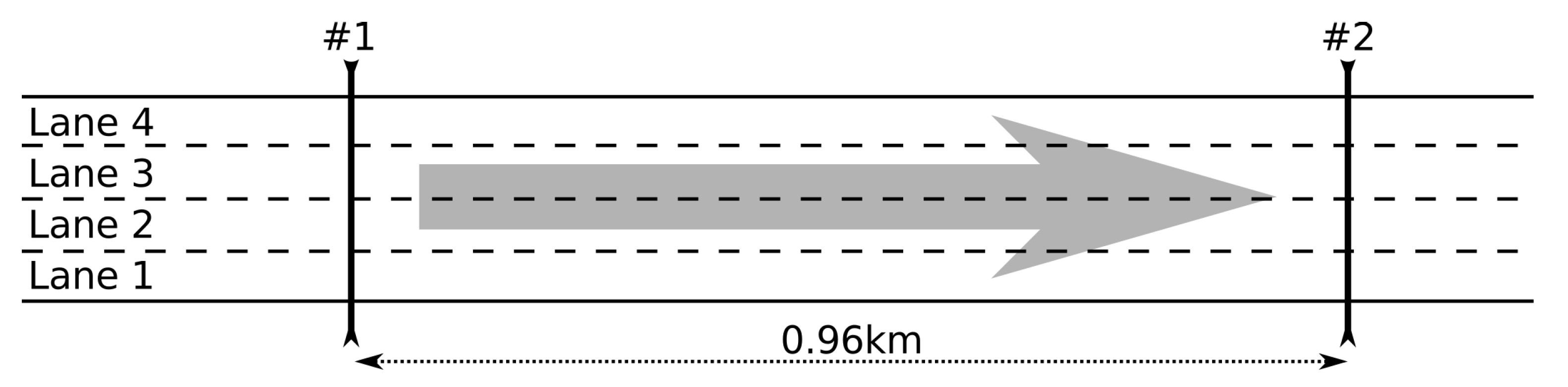
To verify the proposed model, we carried out numerical experiments using traffic detector data for a segment of the I-580 freeway in California, USA, obtained from PeMS ([1]). We used two loop detectors, denoted # 1 and # 2 , separated by 1 km segment of the 4-lane freeway with no entrances or exits, as shown in Figure 2.
The data of the stationary traffic detectors # 1 and # 2 were used to construct the corresponding fundamental diagrams for equilibrium velocity V ( ρ ) . According to the three-phase traffic theory ([17]), the following traffic phases are distinguished:
  • Free flow: 0 ρ < ρ 1
  • Synchronized flow: ρ 1 ρ < ρ 2
  • Wide moving jam: ρ 2 ρ ρ max
For each phase, we define separate functions V ( ρ ) and c ( ρ ) = ρ V ( ρ ) ρ , stitching them together at the transition points:
  • Free flow: V ( ρ ) = α 2 ρ + α 1 c ( ρ ) = α 2 ρ 0 ρ < ρ 1
  • Synchronized flow: V ( ρ ) = β 2 ρ + β 1 + β 0 ρ c ( ρ ) = β 2 ρ β 0 ρ , ρ 1 ρ < ρ 2
  • Wide moving jam: V ( ρ ) = c * ρ max ρ 1 c ( ρ ) = c * ρ max ρ , ρ 2 ρ ρ max
For the traffic detectors showcased in Figure 2, we have the following coefficients and parameters, aggregated over four lanes of I-580:
detectors # 1 : ρ 1 = 0.084 veh./m, α 1 = 49.6 , α 2 = 293.2 , ρ 2 = 0.141 veh./m, β 0 = 2.49 , β 1 = 4.9 , β 2 = 1.6 , c * = 4.20 m/s, ρ max = 0.58 veh./m;
detectors # 2: ρ 1 = 0.076 veh./m, α 1 = 50.2 , α 2 = 295.7 , ρ 2 = 0.165 veh./m, β 0 = 2.30 , β 1 = 0.4 , β 2 = 27.6 , c * = 3.58 m/s, ρ max = 0.58 veh./m;
For the separate lane of the I-580 freeway, the following parameters are different. For example, in the first lane:
detectors # 1 : ρ 1 = 0.023 veh./m, α 1 = 52.5 , α 2 = 1026.9 , ρ 2 = 0.036 veh./m, β 0 = 0.46 , β 1 = 22.3 , β 2 = 585.5 , c * = 4.57 m/s, ρ max = 0.145 veh./m;
detectors # 2 : ρ 1 = 0.021 veh./m, α 1 = 53.2 , α 2 = 1075.0 , ρ 2 = 0.040 veh./m, β 0 = 0.58 , β 1 = 10.3 , β 2 = 361.6 , c * = 3.96 m/s, ρ max = 0.145 veh./m;
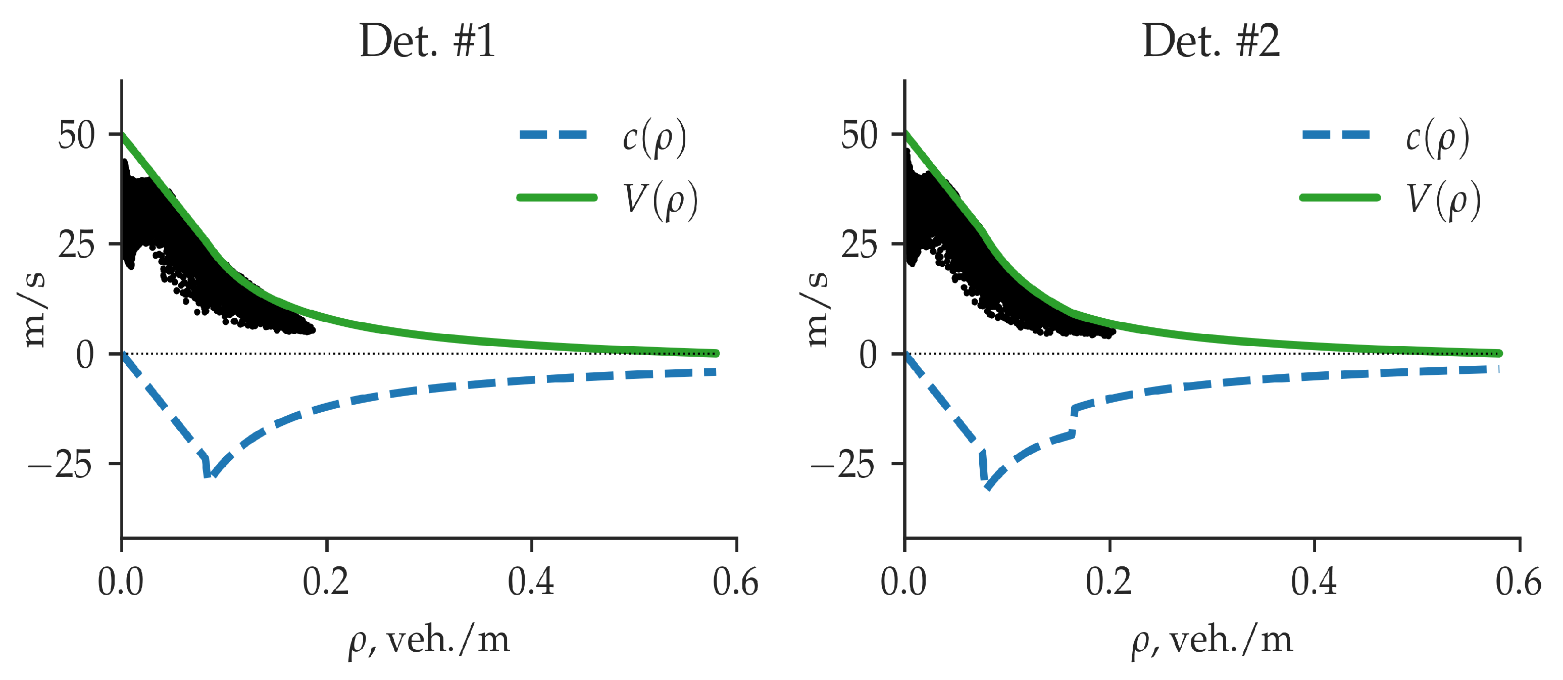
The equilibrium velocity V ( ρ ) — solid green line and the relative velocity of the congestion propagation c ρ = ρ V ( ρ ) ρ — dashed blue line are shown as the functions of density for both detectors, together with the historic data for the one-year period in Figure 3 for the first lane and in Figure 4 aggregated over all four lanes.
Data (traffic flow and velocity, with 30-second temporal resolution) from detector # 1 were used as the initial and left boundary conditions, and data from the downstream detector # 2 
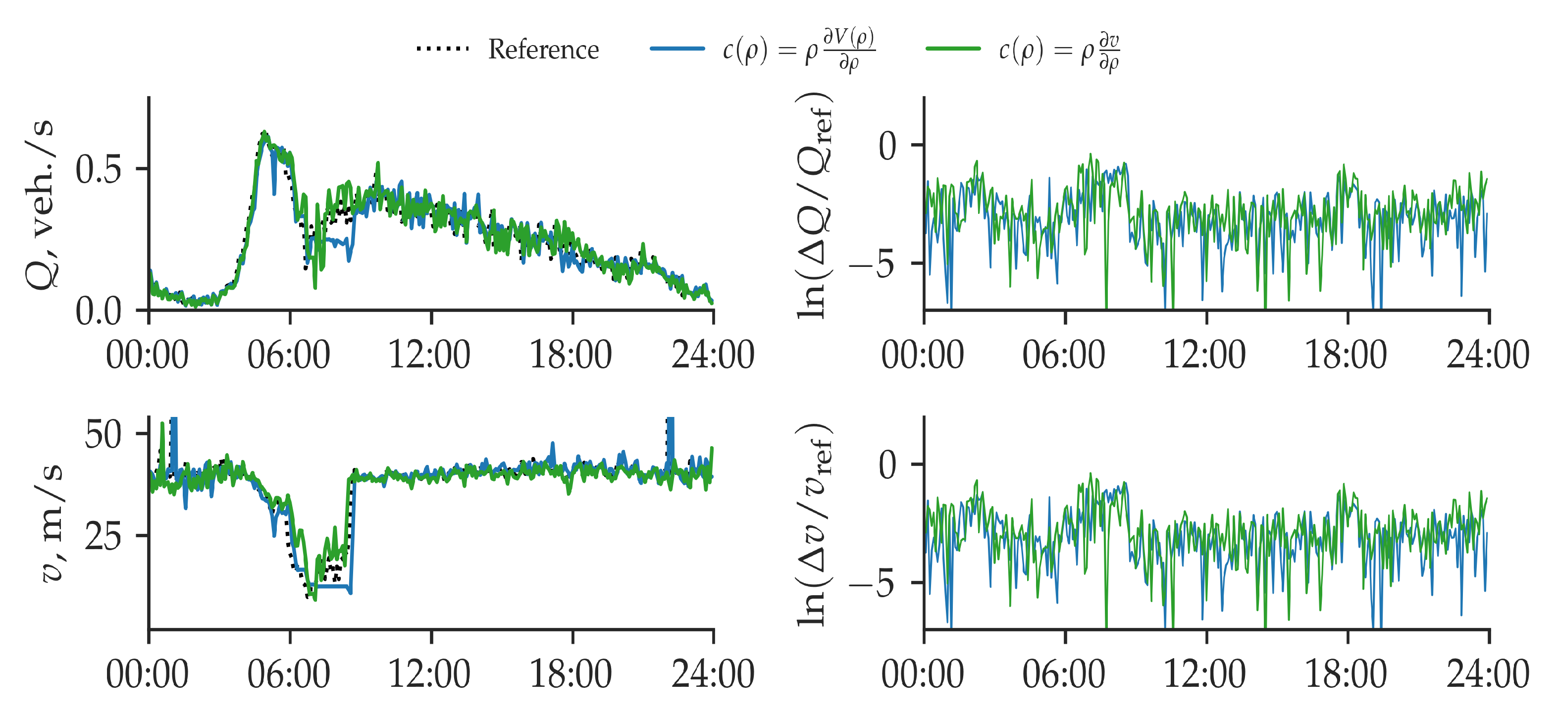
were used for verification of the model output. We simulated a 24-h interval for a single weekday for all lanes of I-580. The results are shown in Figure 5 for the first lane and in 
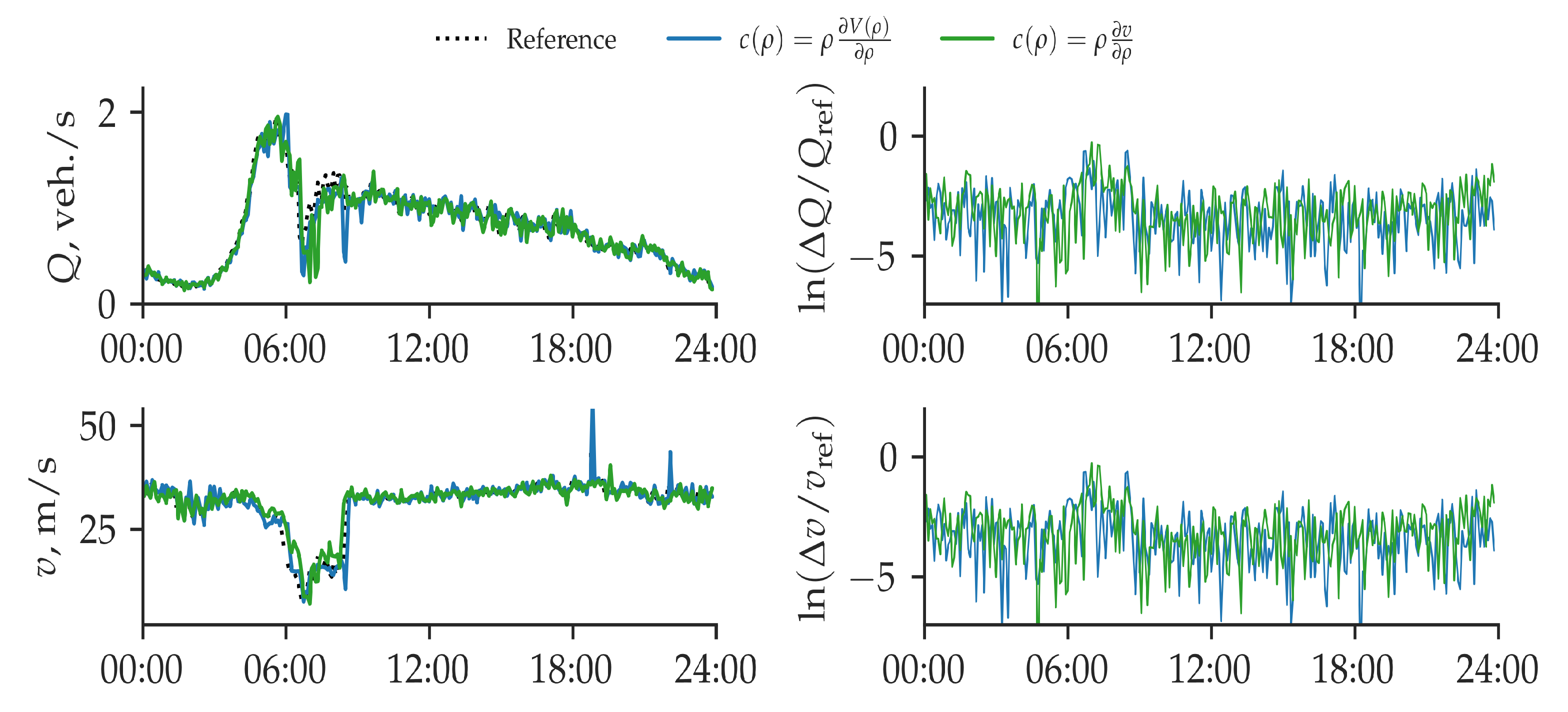
Figure 6 aggregated over four lanes in different subplots: top left, traffic flows; top right, flow relative error in logarithmic scale; bottom left—traffic velocities; bottom right — velocity relative error in the logarithmic scale.
The simulation results obtained with a different expression for the relative velocity of the congestion propagation are shown in different colors: proposed macroscopic second-order model, where we approximate the value of relative velocity of the congestion, c ρ = ρ v ρ , using instantaneous measurements of traffic density and speed (29), is shown in green; the same model (15), with equilibrium velocity c ρ = ρ V ρ ρ as an empirical function of density obtained from the historic detector data, is shown in blue. The reference results (data of detector # 2 ) are depicted by a grey dashed line.
The simulation shows a good but not exact match with the results obtained using the same second-order macroscopic model (15) with a different form of the relative velocity of the congestion propagation, c ( ρ ) . We also see that both approaches have a good match with the reference results.
The root mean square error (RMSE) of velocity for the results of compared models and the detector # 2 measurements in Figure 5 is 0.25406 m/s for the model (15) with c ( ρ ) = ρ V ρ ρ ; and 0.31976 m/s, if c ( ρ ) = ρ v ρ . For the flow, RMSE is 0.00387 veh./s, if c ( ρ ) = ρ V ρ ρ ; and 0.00383 veh./s, if c ρ = ρ v ρ . For the results in Figure 6, velocity RMSE is 0.19646 m/s, if c ( ρ ) = ρ V ρ ρ ; and 0.2331 m/s, if c ( ρ ) = ρ v ρ . The flow RMSE is 0.01237 veh./s if and 0.01301 veh./s, respectively.
The difference in the results between these two approaches come from the time structure. In the first case, we have the continuous empirical function c ( ρ ) = ρ V ρ ρ , with values dependent only on traffic density at each time instant. In the second case, we have a discrete function c ( ρ ) = ρ i n + ρ o u t 2 v o u t v i n ρ o u t ρ i n , with values dependent both on traffic density and velocity. An instant error generally occurs in detector measurements, which is smoothed out in the first case, when we use the fundamental diagram.

5. Conclusions

In this paper, we generalized the second-order hydrodynamic macroscopic traffic models in various formulations [4,5,6,7,8,9,10,11]. Existing second-order macroscopic models describe traffic as non-linear systems of hyperbolic equations (for density and speed), which differ in the way they account for dependency between traffic flow (or velocity) and density. We have shown that all these second-order macroscopic models can be unified using the expression for the relative velocity of the congestion propagation.
To verify the proposed methodology, we conducted numerical experiments by simulating the segment of the I-580 freeway in California, USA, using data from PeMS ([1]). The simulations show that the results obtained for the same macroscopic model when using different forms of the relative velocity of the congestion propagation are slightly different. This suggests that the properties of every phenomenological model are defined by the form of the relative velocity of the congestion propagation—namely, the form of its dependency on density.
It is important to understand why the transition from macroscopic first-order models to second-order models is useful: adding the momentum equation into the system obviates the need for a fundamental diagram. Instead, the relative velocity of the congestion propagation can be obtained from traffic detector measurements. This enables the model to instantly adjust to real-time road conditions.

Author Contributions

Conceptualization, Y.K. and A.K.; methodology, Y.K. and A.A.; software, A.A.; validation, A.A. and V.K.; formal analysis, Y.K. and A.A.; investigation, Y.K. and A.A.; resources, Y.K.; data curation, A.A. and V.K.; writing—original draft preparation, Y.K.; writing—review and editing, Y.K. and A.K.; visualization, A.A. and V.K.; supervision, Y.K.; project administration, Y.K.; funding acquisition, Y.K. All authors have read and agreed to the published version of the manuscript.

Funding

The work was supported by grant RSCF 14-11-00877.

Institutional Review Board Statement

Not applicable.

Informed Consent Statement

Not applicable.

Data Availability Statement

Not applicable.

Conflicts of Interest

The authors declare no conflict of interest.

References

  1. PeMS. 2017. Available online: http://pems.dot.ca.gov (accessed on 17 June 2021).
  2. Lighthill, M.J.; Whitham, G.B. On kinematic waves II. A theory of traffic flow on long crowded roads. Proc. R. Soc. London. Ser. Math. Phys. Sci. 1955, 229, 317–345. [Google Scholar] [CrossRef]
  3. Richards, P.I. Shock Waves on the Highway. Oper. Res. 1956, 4, 42–51. [Google Scholar] [CrossRef]
  4. Payne, H.J. Model of Freeway Traffic and Control; Simulation Councils, Inc.: San Diego, CA, USA, 1971; pp. 51–61. [Google Scholar]
  5. Daganzo, C.F. Requiem for second-order fluid approximations of traffic flow. Transp. Res. Part Methodol. 1995, 29, 277–286. [Google Scholar] [CrossRef]
  6. Papageorgiou, M. Some remarks on macroscopic traffic flow modelling. Transp. Res. Part Policy Pract. 1998, 32, 323–329. [Google Scholar] [CrossRef]
  7. Aw, A.; Rascle, M. Resurrection of “Second Order” Models of Traffic Flow. SIAM J. Appl. Math. 2000, 60, 916–938. [Google Scholar] [CrossRef]
  8. Zhang, H. A non-equilibrium traffic model devoid of gas-like behavior. Transp. Res. Part Methodol. 2002, 36, 275–290. [Google Scholar] [CrossRef]
  9. Zhang, H. Anisotropic property revisited––Does it hold in multi-lane traffic? Transp. Res. Part Methodol. 2003, 37, 561–577. [Google Scholar] [CrossRef]
  10. Siebel, F.; Mauser, W. On the Fundamental Diagram of Traffic Flow. SIAM J. Appl. Math. 2006, 66, 1150–1162. [Google Scholar] [CrossRef] [Green Version]
  11. Siebel, F.; Mauser, W. Synchronized flow and wide moving jams from balanced vehicular traffic. Phys. Rev. E 2006, 73. [Google Scholar] [CrossRef] [PubMed] [Green Version]
  12. Alekseenko, A.; Kholodov, Y.; Kholodov, A.; Chekhovich, Y.; Starozhilets, V. Adaptive Traffic Light Control on Highway Entrances. In Proceedings of the 2017 IEEE 20th International Conference on Intelligent Transportation Systems (ITSC), Yokohama, Japan, 16–19 October 2017; pp. 1–6. [Google Scholar] [CrossRef]
  13. Whitham, G. Linear and Nonlinear Waves; John Wiley & Sons Inc.: New York, NY, USA, 1974. [Google Scholar]
  14. Godunov, S.K.; Romenskii, E.I. Elements of Continuum Mechanics and Conservation Laws; Springer US: New York, NY, USA, 2003. [Google Scholar] [CrossRef] [Green Version]
  15. Helbing, D. Traffic and related self-driven many-particle systems. Rev. Mod. Phys. 2001, 73, 1067–1141. [Google Scholar] [CrossRef] [Green Version]
  16. Magomedov, K.; Kholodov, A. The construction of difference schemes for hyperbolic equations based on characteristic relations. USSR Comput. Math. Math. Phys. 1969, 9, 158–176. [Google Scholar] [CrossRef]
  17. Kerner, B.S. Introduction to Modern Traffic Flow Theory and Control; Springer: Berlin/Heidelberg, Germany, 2009. [Google Scholar] [CrossRef]
Figure 1. Contour bounding an integration cell.
Mathematics 09 02001 g001
Figure 2. Traffic detectors # 1 and # 2 chosen in the segment of the I-580 freeway in California, USA. Data from detector # 1 were used as a left boundary condition for modeling, and data from the downstream detector # 2 were used for the verification of modeling results.
Mathematics 09 02001 g002
Figure 3. Equilibrium speed V ( ρ ) (solid green line) and relative velocity of the congestion propagation c ρ = ρ V ( ρ ) ρ (dashed blue line) as the functions of density for the first lane of I-580 together with the historic data for the one-year period. Left: detector # 1 , right: detector # 2 .
Mathematics 09 02001 g003
Figure 4. Equilibrium speed V ( ρ ) (solid green line) and relative velocity of the congestion propagation c ρ = ρ V ( ρ ) ρ (dashed blue line) as functions of density aggregated over four lanes of I-580, together with the historic data for the one-year period. Left: detector # 1 , right: detector # 2 .
Mathematics 09 02001 g004
Figure 5. The comparison of calculated flows (top) and velocities (bottom) from the first lane of I-580 and observed values from detector # 2 (dashed grey lines). On the right, flow (top) and velocity (bottom) relative errors in logarithmic scale. The simulation results obtained with a different expression for the relative velocity of the congestion propagation, c ρ , are shown in different colors: green, model (with c ( ρ ) = ρ v ρ ρ from (29); blue, the same model (15) with c ( ρ ) = ρ V ρ ρ as an empirical function of density.
Mathematics 09 02001 g005
Figure 6. The comparison of calculated flows (top) and velocities (bottom) aggregated over four lanes of I-580 and observed values from detector # 2 (dashed grey lines). On the right, flow (top) and velocity (bottom) relative errors in logarithmic scale. The simulation results obtained with a different expression for the relative velocity of the congestion propagation, c ( ρ ) , are shown in different colors: green, model (with c ( ρ ) = ρ v ρ ρ from (29); blue, the same model (15) with c ( ρ ) = ρ V ρ ρ as an empirical function of density.
Mathematics 09 02001 g006
Publisher’s Note: MDPI stays neutral with regard to jurisdictional claims in published maps and institutional affiliations.

