Two Gaussian Bridge Processes for Mapping Continuous Trait Evolution along Phylogenetic Trees

Abstract

Gaussian processes are powerful tools for modeling trait evolution along phylogenetic trees. As the value of a trait may change randomly throughout the evolution, two Gaussian bridge processes, the Brownian bridge (BB) and the Ornstein–Uhlenbeck bridge (OUB), are proposed for mapping continuous trait evolution for a group of related species along a phylogenetic tree, respectively. The corresponding traitgrams to the two bridge processes are created to display the evolutionary trajectories. The novel models are applied to study the body mass evolution of a group of marsupial species.

1. Introduction

Evolution is the change in the heritable traits of biological populations over successive generations [1]. Evolution occurs ubiquitously on our planet because all species need to survive by adapting themselves to the living environment. For phenotypic evolution, the trait value, such as body mass, may change across generations in the evolutionary history. Scientists use mathematical models and computing tools to describe the behavior of change in trait evolution. In particular, the change of a trait value for a species can be modeled by a stochastic variable of continuous type varying with time.

Let the stochastic variable $x_t$ be a species’ trait value at time t, $x_t$ solves the one-dimensional stochastic differential Equation (SDE) in Equation (1)

$$d{x}_t=b(x_t,t,\mathrm{\Theta })dt+\sigma (x_t,t,\mathrm{\Theta })d{W}_t,x\left(0\right)=x_0,$$

(1)

where $d{x}_t$ is the infinitesimal change in the character x over the infinitesimal interval from time t to time $t+dt$, $b(x_t,t,\mathrm{\Theta })$ is called the drift coefficient, $b(x_t,t,\mathrm{\Theta })dt$ measures the deterministic trait value in an infinitesimal time, $\sigma (x_t,t,\mathrm{\Theta })$ is the diffusion coefficient, $\sigma (x_t,t,\mathrm{\Theta })dt$ measures the change as a result of random perturbations in an infinitesimal time, $W_t$ is a Wiener process starting from $W\left(0\right)=0$ with an independent Gaussian increment $W\left(t\right)-W\left(s\right)$ of mean 0 and variance $t-s$, and $\mathrm{\Theta }$ is a parameter vector (see [2,3]).

In the family of stochastic processes, the Brownian motion (BM) [4,5,6] and the Ornstein-Uhlenbeck (OU) processes [2,3,7] are the two most popular Gaussian processes for modeling trait evolution. A Brownian motion trait variable $x_t$ without the drift effect (i.e., $b(x_t,t,\mathrm{\Theta })=0$) and with $\sigma (x_t,t,\mathrm{\Theta })=\sigma$ solves the SDE in Equation (2)

$$d{x}_t=\sigma d{W}_t,$$

(2)

and due to the property of the Winer process, the variation of $x_t$ is proportional to time (i.e., $\mathrm{Var}\left(x_t\right)={\sigma }^{2}t$), where the positive parameter $\sigma$ is regarded as the rate of evolution.

When treating $x_t$ followed as an OU stochastic variable (i.e., $b(x_t,t,\mathrm{\Theta })=\alpha (\theta -x_t)$ and $\sigma (x_t,t,\mathrm{\Theta })=\sigma$) [7], the corresponding trait variable $x_t$ solves the SDE in Equation (3)

$$d{x}_t=\alpha (\theta -x_t)dt+\sigma d{W}_t,$$

(3)

where the deterministic term $\alpha (\theta -x_t)dt$ is interpreted as the force of selection [2], $\alpha >0$ measures the strength of selection, $\theta \in \mathcal{R}$ is the long-term mean level optimum of the trait, $\theta -x_t$ measures the distance of the current trait value $x_t$ from the optimum $\theta$, and $\sigma >0$ is the rate of evolution, as defined earlier for the Brownian motion. In particular, when the force parameter $\alpha$ is 0, the OU process reduces to the Brownian motion.

For studying the trait evolution for a group of related species, scientists apply the phylogenetic comparative methods (PCMs) to understand their evolutionary history [5,8,9,10]. PCMs incorporate phylogenetic trees (acylic-directed diagrams that represent the evolutionary history) to analyze phenotypic data. For instance, an ornithologist applies PCMs to study the evolutionary divergence of waterfowl (e.g., swan) and sea-fowl (e.g., sea gull) by investigating their common traits (e.g., wing shape, flight speed, or/and wing span length) [11], while an evolutionary biologist uses PCMs to study the primate evolution by comparing their body size and brain size [12]. PCMs can also be applied to estimate the rate of evolution [6,13], estimate the ancestral status [8,14], test the evolutionary phylogenetic signal [15,16], and detect the evolutionary correlation among traits [17,18].

This work aims to provide a tool for exploring the evolutionary trajectories built along a given phylogenetic tree with known topology and branch lengths and the traits observed at the tips of the tree. The procedure starts at the tips of the tree with known trait data and works backwards up the tree to fill in trait values at early branching points. Then, by conditioning these known internal values, a bridge process is applied to simulate trajectories. Two Gaussian bridge processes, the Brownian bridge process and the Ornstein–Uhlenbeck bridge, are introduced for this purpose herein. The goal of this work is two-fold: first, the new method generates a stochastic map under a bridge process to provide an overview of the entire change for a group of species; second, the new method creates a traitgram that allows the fluctuation of trait changes along the branch of the phylogenetic tree. Note that Revell [19] presented graphical methods for visualizing both the discrete and continuous phenotypic evolution along a phylogenetic tree. While Revell [19] used a weighted average method to generate the map where change of trait value was changed monotonically in an increase/decrease manner, our work implements bridge processes to allow random changes of the trait value.

The background and implementation of the two bridge processes to model trait evolution along the phylogenetic tree are provided in Section 2. The results are shown in Section 3, where simulation results for assessing the new models is provided in Section 3.1, and analysis of an empirical dataset using the traitgrams can be accessed in Section 3.2. The conclusion and discussion of this work are provided in Section 4 and Section 5, respectively.

2. Methods

2.1. Bridge Process

The bridge process is a member of the continuous-type stochastic process family. Formally, a bridge process’ random variable $y_t$ has a starting value a at time $t=t_0$ and an end value b at a known time $t=T$. A bridge process with the initial condition $y\left(t_0\right)=a$ at $t=t_0$ can be constructed by conditioning on $y_T$ and yields to a fixed value of b at time $t=T$.

A bridge process random variable $y_t$ solves the SDE in Equation (4)

$$d{y}_t=c_T(y_t,t,\mathrm{\Theta })dt+\sigma (y_t,t,\mathrm{\Theta })d{W}_t,y\left(0\right)=a,$$

(4)

where $c_T(y_t,t,\mathrm{\Theta })$ is the drift coefficient of $y_t$, and $\sigma (y_t,t,\mathrm{\Theta })$ is the diffusion coefficient of $y_t$.

Szavits–Nossan and Evans [20] expressed $c_T(y_t,t,\mathrm{\Theta })$ in terms of the drift coefficient $b(x_t,t,\mathrm{\Theta })$ and the diffusion coefficient $\sigma (x_t,t,\mathrm{\Theta })$, defined in Equation (1), as the following,

$$c_T(x,t,\mathrm{\Theta })=b(x,t,\mathrm{\Theta })+{\sigma }^2(x,t,\mathrm{\Theta })\frac{\partial }{\partial x}logp(b,T|x,t,\mathrm{\Theta }),$$

(5)

where $p(b,T|x,t,\mathrm{\Theta })$ is the transition density function of $x_t$ corresponding to the stochastic differential equation in Equation (1). Furthermore, $p(x,t|x^{\prime },t^{\prime })$ solves the Fokker–Planck equation (forward Kolmogorov equation)$\frac{\partial p(x,t|0,0)}{\partial t}$ = $-\frac{\partial }{\partial x}\left[b(x,t)p(x,t|0,0)\right]$ + $\frac{1}{2}\frac{{\partial }^2}{{\partial }^{2}x}\left[\sigma (x,t)p(x,t|0,0)\right]$ subject to the initial condition $p(x,t|a,0)=\delta (x-a)$, a Dirac delta function.

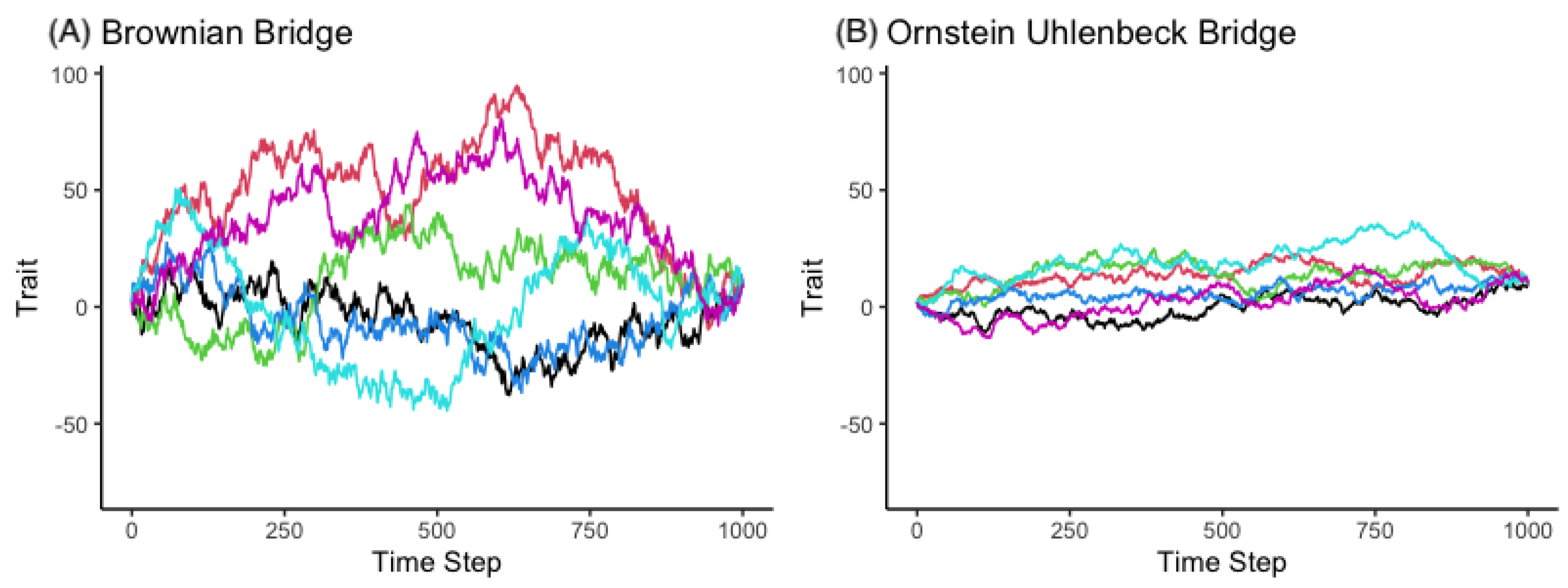
2.1.1. The Brownian Bridge

The Brownian bridge is a well-known continuous-time stochastic process defined as $y_t:=\left(W_t\right|W_0=a,W_T=b),t\in [0,T]$, where $W\left(t\right)$ is a Wiener process with $W_0=a$ and an independent Gaussian increment and continuous paths. In the literature, the Brownian bridge has been broadly applied in many fields. For instance, Buchin et al. [21] used the Brownian bridge to study the linear movement between sample points under the circumstance that the trajectory data are with high uncertainty.

Since the probability density p for the Brownian motion to the Fokker–Plank equation subject to $p(x,t|a,0)=\delta (x)$ is given by

$$p(x,t|0,0)=\frac{1}{\sigma \sqrt{2\pi t}}\exp \left(-\frac{x^2}{2{\sigma }^{2}t}\right),$$

(6)

and due to the process being both space and time homogeneous for the Brownian motion, the expression for $p(b,T|x,t)$ is the same as for $p(b-x,T-t|0,0)$, implying

$$p(b,T|x,t)=\frac{1}{\sigma \sqrt{2\pi (T-t)}}\exp \left(-\frac{{(b-x)}^2}{2{\sigma }^2(T-t)}\right).$$

(7)

Using Equation (5) and adopting the derivation in [20], the coefficient $c_T$ for the Brownian bridge is shown in Equation (8)

$$c_T(x,t)=0+{\sigma }^2\frac{\partial }{\partial x}log\left(\frac{1}{\sigma \sqrt{2\pi (T-t)}}·\exp \left(-\frac{{(b-x)}^2}{2{\sigma }^2(T-t)}\right)\right)=\frac{b-x}{T-t}.$$

(8)

Hence, the Brownian bridge random variable $y_t$ solves the SDE in Equation (9)

$$d{y}_t=\frac{b-y_t}{T-t}dt+\sigma d{W}_t,y\left(0\right)=a.$$

(9)

The solution of Equation (9) can be obtained by the variation of constants method [22] and is shown in Equation (10)

$$y_t=a(1-\frac{t}{T})+b\frac{t}{T}+\sigma (T-t){\int }_0^t\frac{1}{T-s}d{W}_s.$$

(10)

Equation (10) is used to simulate the trajectory given the starting and end values under the Brownian bridge.

Take the expectation of $y_t$ and $y_t^2$ and using the Itô isometry property, the expected value and variance of $y_t$ are shown in Equation (11) and Equation (12), respectively.

$$E\left[y_t\right]=a+(b-a)\frac{t}{T},$$

(11)

and

$$Var\left(y_t\right)={\sigma }^2\frac{t(T-t)}{T}.$$

(12)

Note that Equation (12) implies that the most uncertainty is in the middle of the bridge, with zero uncertainty at the nodes.

2.1.2. The OU Bridge

The OU bridge [20] can be constructed by utilizing the transition density of the OU process given in Equation (13).

$$p(x,t|0,0)=\frac{1}{\sigma \sqrt{2\pi \kappa (\alpha ,t)}}\exp \left(-\frac{{(x-\theta (1-\exp (-\alpha t)))}^2}{2{\sigma }^2\kappa (\alpha ,t)}\right),$$

(13)

where $\kappa (\alpha ,t)=\frac{1-\exp (-2\alpha t)}{2\alpha }$.

The expression of $p(b,T|x,t)$ is shown in Equation (14)

$$p(b,T|x,t)=\frac{1}{\sigma \sqrt{2\pi \kappa (\alpha ,(T-t\left)\right)}}\exp \left(-\frac{{(b-\theta -(x-\theta )\exp \left(-\alpha (T-t)\right))}^2}{2{\sigma }^2\kappa (\alpha ,(T-t))}\right).$$

(14)

Using Equation (5) with $b(x,t)=\alpha (\theta -x)$ and $\sigma (x,t)=\sigma$, the drift coefficient $c_T$ for the Ornstein–Uhlenbeck bridge subject to $p(x,0|a,0)=\delta (x)$ solves the forward Kolmogorov equation and is expressed in Equation (15)

$$\begin{array}{cc}\hfill c_T(x,t)& =\alpha (\theta -x)+{\sigma }^2\frac{\partial }{\partial x}logp(b,T|x,t)\hfill \\ & =\alpha (\theta -x)+\frac{[b-\theta -(x-\theta \left)\exp \right(-\alpha (T-t)\left)\right]\exp (-\alpha (T-t\left)\right)}{\kappa (\alpha ,T-t)}.\hfill \end{array}$$

(15)

Note that when $\alpha$ approaches 0, it can be algebraically verified that the $c_T(x,t)$ in Equation (15) for the OU bridge converges to the $c_T(x,t)$ in Equation (8) for the Brownian bridge.

The stochastic differential equation for the OU bridge is thus given by   

$$d{y}_t=\left[\alpha (\theta -y_t)+\frac{[b-\theta -(y_t-\theta )\exp (-\alpha (T-t))]\exp (-\alpha (T-t))}{\kappa (\alpha ,T-t)}\right]dt+\sigma d{W}_t,y\left(0\right)=a,$$

(16)

which can be simplified into   

$$d{y}_t+\alpha coth\left(\alpha (T-t)\right)y_{t}dt=\{\alpha (b-\theta )csch\left(\alpha (T-t)\right)+\theta coth\left(\alpha (T-t)\right)\}dt+\sigma d{W}_t,y\left(0\right)=a,$$

(17)

where coth and csch are hyperbolic tangent and hyperbolic cosecant functions, respectively.

The solution $y_t$ to the Equation (17) for the OU bridge can be obtained by applying the variation of constants method by two steps [22]. First, the homogeneous solution of Equation (17) can be obtained by solving the first-order linear differential equation

$$d{y}_t+\alpha coth\left(\alpha (T-t)\right)y_{t}dt=0.$$

(18)

The ordinary differential equation in Equation (18), given $y\left(0\right)=a$, has the solution

$$y_c\left(t\right)=\frac{a}{sinh\left(\alpha T\right)}sinh\left(\alpha (T-t)\right).$$

(19)

Second, the particular solution $y_p\left(t\right)=k\left(t\right)sinh\left(\alpha (T-t)\right)$ for Equation (17) can be obtained by solving   

$$d{y}_p\left(t\right)+\alpha coth\left(\alpha (T-t)\right)y_p\left(t\right)dt=\alpha (b-\theta )csch\left(\alpha (T-t)\right)dt+\theta coth\left(\alpha (T-t)\right)dt+\sigma d{W}_t.$$

(20)

which yield the solution   

$$y_p\left(t\right)=(b-\theta )\frac{sinh\left(\alpha t\right)}{sinh\left(\alpha T\right)}+\theta \left[1-\frac{sinh\left(\alpha \right(T-t\left)\right)}{sinh\left(\alpha T\right)}\right]+\sigma sinh\left(\alpha (T-t)\right){\int }_0^t\frac{1}{sinh\left(\alpha \right(T-s\left)\right)}d{W}_s.$$

(21)

Therefore, the full solution for the OU bridge in Equation (17) is

$$y\left(t\right)=y_c\left(t\right)+y_p\left(t\right).$$

(22)

Taking the expectation of $y_t$ and $y_t^2$ and using the Itô isometry property, the expected value and the variance of $y_t$ are

$$E\left[y_t\right]=a\frac{sinh\left(\alpha \right(T-t\left)\right)}{sinh\left(\alpha T\right)}+(b-\theta )\frac{sinh\left(\alpha t\right)}{sinh\left(\alpha T\right)}+\theta \left[1-\frac{sinh\left(\alpha \right(T-t\left)\right)}{sinh\left(\alpha T\right)}\right],$$

(23)

and

$$Var\left(y_t\right)={\sigma }^2{sinh}^2\left(\alpha (T-t)\right){\int }_0^t{csch}^2\left(\alpha (T-s)\right)ds.$$

(24)

Note that the OU bridge also reduces to the Brownian bridge when the force $\alpha$ approaches zero. This property can be algebraically verified by directly computing the limit of the first two moments (${lim}_{\alpha \to 0}{E}_{\mathrm{OU}}\left[y_t\right]=E_{\mathrm{BM}}\left[y_t\right]$ and ${lim}_{\alpha \to 0}Va{r}_{\mathrm{OU}}\left[y_t\right]=Va{r}_{\mathrm{BM}}\left[y_t\right]$). Therefore, $E\left[y_t\right]$ in Equation (23) converges to $E\left[y_t\right]$ in Equation (11), and $Var\left[y_t\right]$ in Equation (24) converges to $Var\left[y_t\right]$ in Equation (12), respectively.

Sample paths for the Brownian bridge and for the Ornstein–Uhlenbeck bridge are shown in Figure 1.

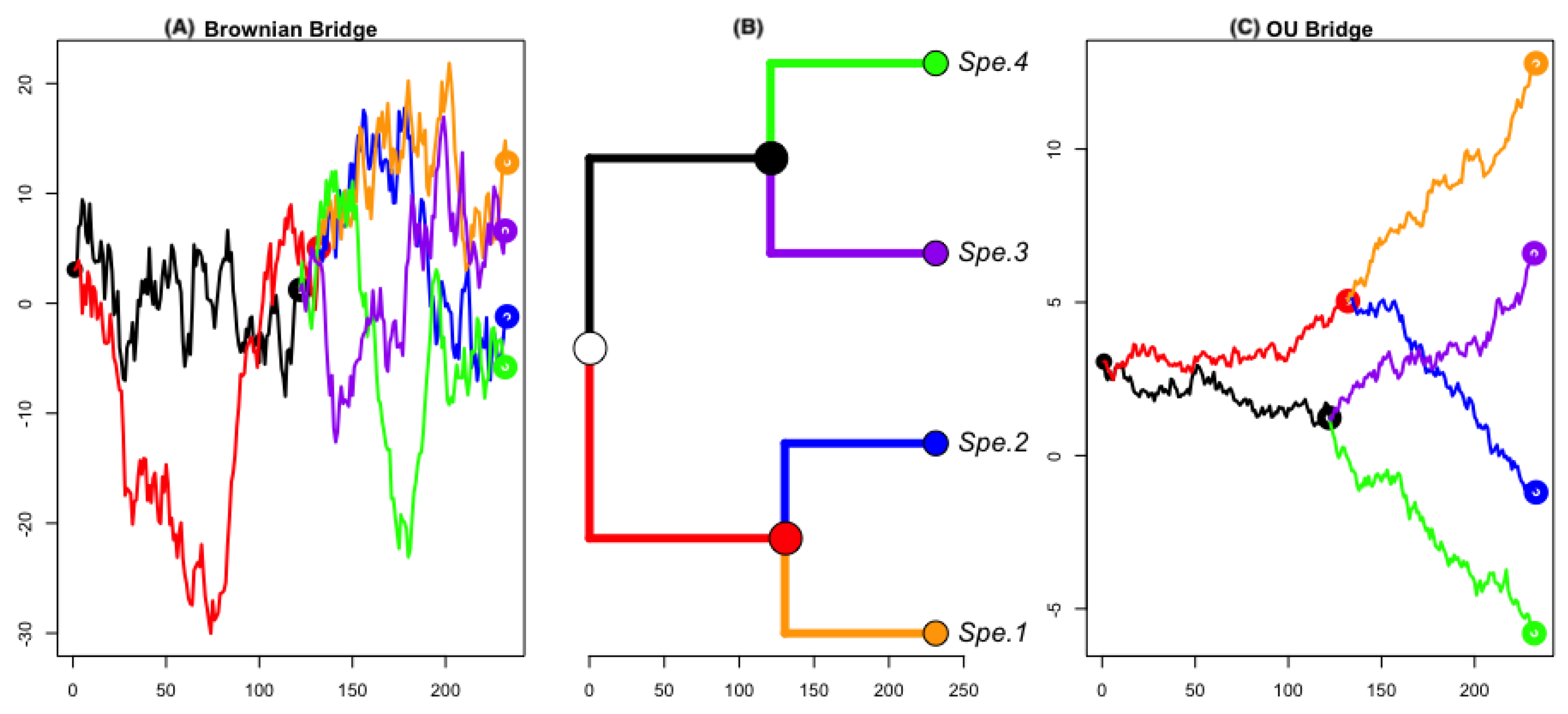
2.2. Bridge Process along Phylogenetic Tree

In this section, we implement the bridge process for trait evolution along a root phylogenetic tree. A rooted phylogenetic tree $\mathcal{T}$ has a fixed topology equipped with branch lengths that are represented as evolutionary times (e.g., the six horizontal lengths ${\nu }_1,\cdots ,{\nu }_6$ shown in the Figure 2B). Let ${\left\{{\nu }_k\right\}}_{k=1}^m$ be the set of branches, where m is the number of branches and let ${\mathit{Y}}_t={(y_{1,t},y_{2,t},\cdots ,y_{n,t})}^T$ be a stochastic trait vector of n species with the dependency described by the tree topology. To implement the bridge process for trait evolution, each branch ${\nu }_k$ is first divided into fine grids. Denote the integer $N_k,k=1,2,\cdots ,m$ as the number of grids on the kth branch. Samples of $y_t$ are then drawn from the path space of the discrete version of Equation (4). Here, the Euler–Maruyama method [23] is used to approximate the numerical solution of the SDE in Equation (4), which is shown in Equation (25)

$$y_{i+1}=y_i+c_T(y_i,t_i,\mathrm{\Theta }){\Delta }_i+\sigma (y_i,t_i,\mathrm{\Theta })\Delta W_i,$$

(25)

where ${\Delta }_i=t_{i+1}-t_i$, $\Delta W_i=W_{i+1}-W_i$; $c_T(y_i,t_i,\mathrm{\Theta })=\frac{b-y_i}{t_{i+1}-t_i}$, $\sigma (y_i,t_i,\mathrm{\Theta })=\sigma$ for the Brownian bridge model, and $\alpha (\theta -y_i)+\frac{[b-\theta -(y_i-\theta )\exp (-\alpha (t_{i+1}-t_i))]\exp (-\alpha (t_{i+1}-t_i))}{\kappa (\alpha ,t_{i+1}-t_i)}$, $\kappa (\alpha ,t_{i+1}-t_i)=\frac{1-\exp (-2\alpha (t_{i+1}-t_i))}{2\alpha }$ and $\sigma (y_i,t_i,\mathrm{\Theta })=\sigma$ for the OU bridge model.

We then use Equation (25) to generate the trajectories of ${\left\{y_i\right\}}_{i=1}^{N_k}$ on each branch constraint on the topology of the tree $\mathcal{T}$. Sample paths generated under the bridge models along a four-taxa balanced phylogenetic tree is shown in Figure 2.

Prior to generating the full trajectories along the tree, trait values at the internal nodes of the tree are required. Then, the bridge process can be applied therein on each branch. Since only the tree and the trait value observed at the tip (${\mathit{Y}}_{\mathrm{tip}}={(y_1,y_2,\cdots ,y_n)}^T$) are available, we obtained samples of the internal nodes as follows [24,25,26]: Let ${\mathit{Y}}_{\mathrm{node}}$ be the trait vector of internal nodes, and let $\mathrm{\Sigma }$ be the covariance matrix of the trait vector ${\mathit{Y}}_{\mathrm{full}}=({\mathit{Y}}_{\mathrm{tip}},{\mathit{Y}}_{\mathrm{node}})$, represented as

$$\mathrm{\Sigma }=\left(\begin{array}{cc}{\mathrm{\Sigma }}_{\mathrm{tip}}& {\mathrm{\Sigma }}_{\mathrm{tip},\mathrm{node}}\\ {\mathrm{\Sigma }}_{\mathrm{node},\mathrm{tip}}& {\mathrm{\Sigma }}_{\mathrm{node}}\end{array}\right),$$

(26)

where those $\mathrm{\Sigma }$s in the RHS of Equation (26) can be determined according to the corresponding model of trait evolution. Since the joint distribution of ${\mathit{Y}}_{\mathrm{full}}$ under the bridge model is unknown, we instead using the Brownian motion (BM) model and Ornstein–Uhlenbeck (OU) model to obtain the estimates of the internal nodes [27,28]. For the BM model, $\mathrm{\Sigma }=[{\sigma }_{ij}^2]={\sigma }^2{g}_{ij}$, where $g_{ij}$ is the element representing the shared branch length between a pair of nodes. For the OU model, $\mathrm{\Sigma }=\left[{\sigma }_{ij}^2\right]={\sigma }^2\exp (-2\alpha (1-g_{ij}))(1-\exp (-2\alpha g_{ij}))/\left(2\alpha \right)$, where $\alpha >0$ is the force parameter [29,30]. Since both the BM model and the OU model are multivariate normal, the distribution of ${\mathit{Y}}_{\mathrm{node}}$ conditioned on ${\mathit{Y}}_{\mathrm{tip}}$ is again a normal distribution, as shown in Equation (27)

$${\mathit{Y}}_{\mathrm{node}}|{\mathit{Y}}_{\mathrm{tip}}\sim \mathrm{MVN}({\mu }_{\mathrm{tip}},{\mathrm{\Sigma }}_{\mathrm{tip}}),$$

(27)

where

$${\mu }_{\mathrm{node}}={\mu }_{\mathrm{tip}}+{\mathrm{\Sigma }}_{\mathrm{tip},\mathrm{node}}{\mathrm{\Sigma }}_{\mathrm{tip}}^{-1}({\mathit{Y}}_{\mathrm{tip}}-{\mu }_{\mathrm{tip}})\mathrm{and}{\mathrm{\Sigma }}_{\mathrm{node}}={\mathrm{\Sigma }}_{\mathrm{tip}}-{\mathrm{\Sigma }}_{\mathrm{node},\mathrm{tip}}{\mathrm{\Sigma }}_{\mathrm{tip}}^{-1}{\mathrm{\Sigma }}_{\mathrm{tip},\mathrm{node}}.$$

(28)

Hence, given the tip ${\mathit{Y}}_{\mathrm{tip}}$ and tree $\mathcal{T}$, samples of ${\mathit{Y}}_{\mathrm{node}}$ can be drawn accordingly. Since the tree topology represents the dependency of the trait variable, the simulation starts from the root node of the tree and adopts the tree traversal algorithm [31], where one-dimensional bridge process is applied to generate the trajectories on each branch.

3. Result

3.1. Simulation

The simulation is used to describe the state space of $y_t$ given the known parameters $\mathrm{\Theta }$ on each branch of the tree. Balanced trees and comb trees of $4, 8, 32, 64$, and 128 taxa were generated by the R ape package [32]. Trait vectors at the tips ${\mathit{Y}}_{\mathrm{tips}}$ of the tree were simulated using fastBM in the R package phytools [19] with rate parameter $\sigma =1$ and root value $\mu =0$ under the BM model for the Brownian bridge model and with parameters $\alpha =0.05,\theta =1,\sigma =1.85$, and root $\mu =0$ under the OU model for the OU bridge model. The internal node state $Y_{\mathrm{node}}$ is then estimated using Equation (28). For each size of tree, 1000 trajectories are simulated on each branch. Below, we report the simulation results for the 4 taxa case for the left tree case. The results of the balanced tree using taxa $8, 32, 64, 128$ and the results of comb tree using taxa $4, 8, 32, 64, 128$ can be accessed through the link listed in Appendix A.1.

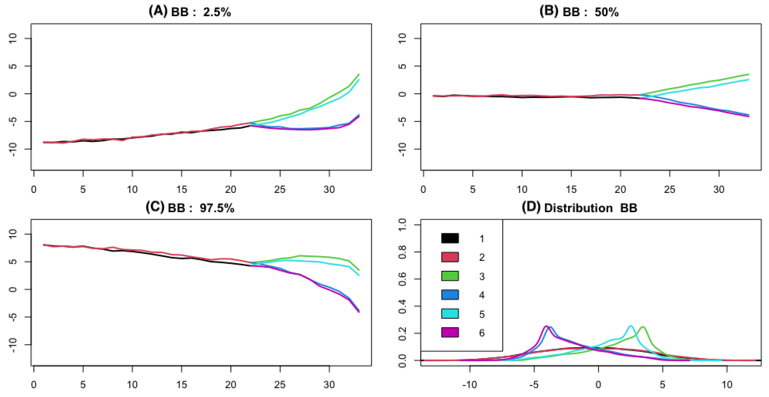
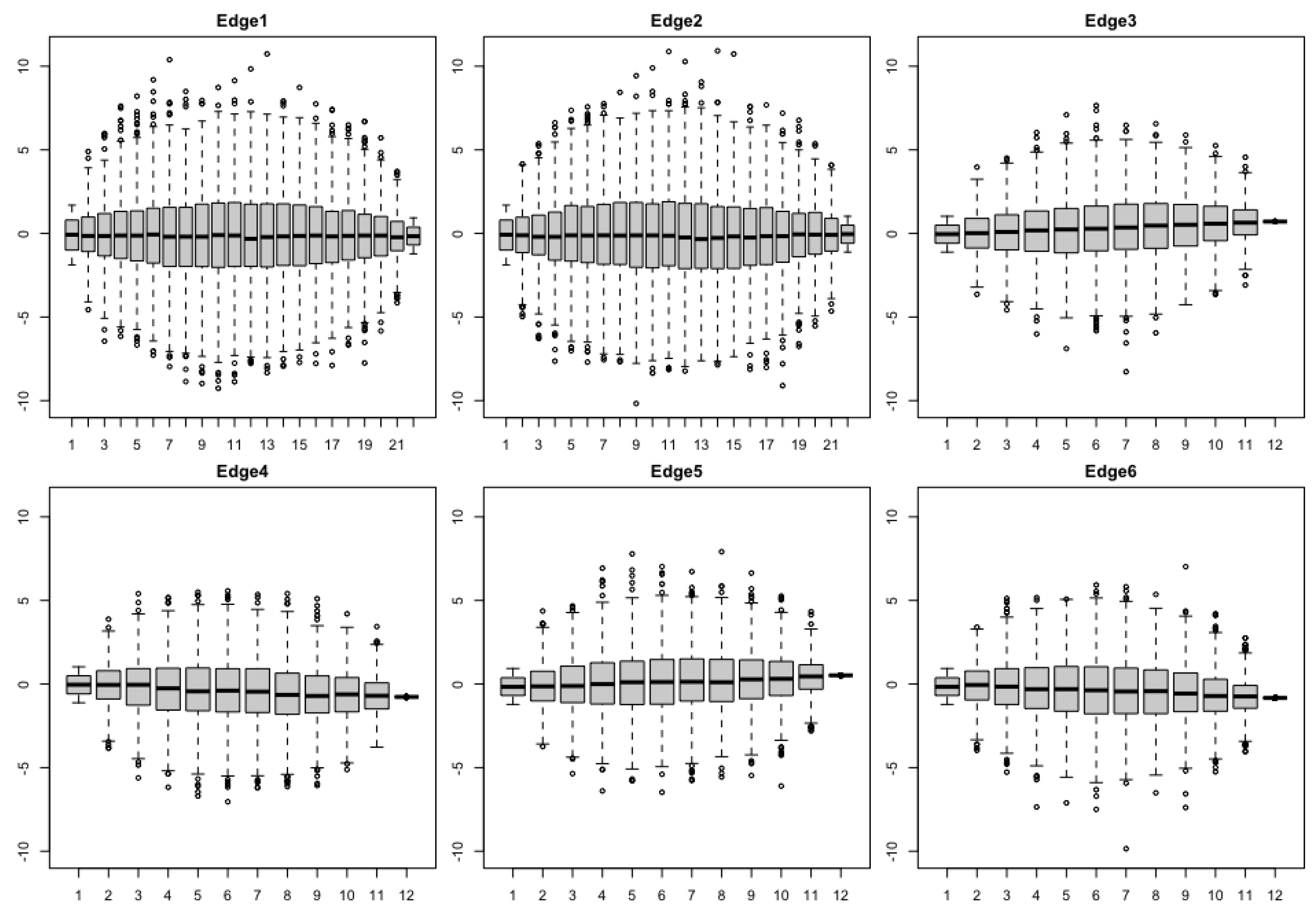
3.1.1. The Brownian Bridge Model

The distribution of the trajectories under the Brownian bridge model for each branch of the four taxa balanced tree is reported by the 2.5%, 50%, and 97.5% level trajectories, the density plots in Figure 3, summary statistics in

Table 1. Summary statistics for the trajectories simulated under the Brownian bridge model using a balanced tree of 4 taxa. Each row of the Table represents the results in the branch corresponding to the branch number in Figure 3 bottom right panel. The last row is the summary statistics for all trajectories. The Min., 1st Qu., Median, Mean, 3rd Qu., Max., sd., skewness, and kurtosis are reported in each column, respectively.

	Min	1st Qu.	Median	Mean	3rd Qu.	Max.	sd	skewness	kurtosis
br1	−12.842	−3.382	−0.580	−0.584	2.216	11.676	3.846	0.008	2.522
br2	−12.106	−3.245	−0.349	−0.345	2.615	10.770	3.945	−0.020	2.417
br3	−6.202	0.097	2.208	1.646	3.506	8.484	2.500	−0.695	2.929
br4	−9.297	−3.812	−2.541	−2.018	−0.454	6.123	2.466	0.662	2.985
br5	−8.042	−0.601	1.361	0.898	2.560	8.592	2.421	−0.628	3.029
br6	−9.762	−4.107	−2.878	−2.362	−0.899	6.092	2.443	0.700	3.030
full	−12.842	−3.204	−0.474	−0.462	2.293	11.676	3.467	0.004	2.469

, and the boxplots in Figure 4.

Table 1 reports the summary statistics of the trajectories on each branch under the Brownian bridge model. From Table 1, the trajectories on each branch vary widely, as the difference between the Min and Max of the samples are large on each branch. This result is also supported by the sd column where the values of the standard deviation are considerably large ($sd=2.421$ for branch 5 and $sd=3.945$) when comparing with the $\sigma =1$ used for simulation.

The skewness computed by $b_1=\left(\frac{1}{nS}{\sum }_{s=1}^S{\sum }_{i=1}^n(y_{is}-{\overline{y}}_s)\right)/\left(\frac{1}{nS-1}{\sum }_{s=1}^S{\sum }_{i=1}^n{(y_{is}-{\overline{y}}_s)}^{3/2}\right)$ and the kurtosis computed by $g_2=\left(\frac{1}{nS}{\sum }_{s=1}^S{\sum }_{i=1}^n{(y_{is}-{\overline{y}}_s)}^4\right)/{\left(\frac{1}{nS}{\sum }_{s=1}^S{\sum }_{i=1}^n{(y_{is}-{\overline{y}}_s)}^2\right)}^2$ using $S=1000$ replicates for the six branches are reported in Table 1. In this trial, the distributions of trajectories under the Brownian Bridges model for branch 1 (black: from time 0 until branching) and for branch 2 (red: from time 0 until branching) are more symmetric ($b_1\approx 0$) but platykurtic ($g_2<3$), for branch 3 (green) and branch 5 (sky blue) are negative skew ($b_1<0$) and kurtic ($g_2\approx 3$), and of branch 4 (blue) and branch 6 (purple) are positive skew ($b_1>0$) and kurtic ($g_2\approx 3$). The skewness for all samples is $0.004$ and the kurtosis for all samples is $2.469$ meaning that the distribution of the trajectories under the Brownian bridge model is symmetric and platykurtic (less outliers are produced than the normal distribution).

Figure 4 shows the boxplots of the trajectories of each branch for the four-taxa balanced tree. On each panel, it can be seen that from the leftmost to the middle then to the rightmost, the interquartile range (IQR: the height of the gray box) increases and reaches its maximum at the middle, then decreases. This indicates that the samples have the largest range drawn in the middle stage compared to samples drawn from other stages. The result is concordant with the property of the Brownian bridge that the middle accounts for the most uncertainty.

3.1.2. The OU Bridge Model

The distribution of the trajectories under the Ornstein–Uhlenbeck model for each branch of the four-taxa balanced tree is reported by the 2.5%, 50%, and 97.5% level trajectories, the density plots in Figure 5, summary statistics in

Table 2. Summary statistics for the trajectories simulated under the Ornstein–Uhlenbeck bridge model using a balanced tree of 4 taxa. Each row of the Table represents the results in the branch corresponding to the branch number in Figure 5 bottom right panel. The last row is the summary statistics for all trajectories. The Min., 1st Qu., Median, Mean, 3rd Qu., Max., sd., skewness, and kurtosis are reported in each column, respectively.

	Min	1st Qu.	Median	Mean	3rd Qu.	Max.	sd	skewness	kurtosis
br1	−1.816	1.074	1.599	1.623	2.282	5.063	0.856	−0.004	3.005
br2	−2.699	0.029	0.539	0.555	1.140	4.071	0.843	0.036	3.194
br3	−2.617	0.083	0.877	0.878	1.679	4.165	0.925	−0.028	2.623
br4	−4.150	−1.856	−0.986	−0.977	−0.084	2.472	1.009	0.017	2.310
br5	−1.359	1.927	2.349	2.358	2.750	5.396	0.751	−0.124	4.078
br6	−0.653	1.935	2.354	2.367	2.772	6.497	0.758	−0.068	3.884
full	−4.150	0.182	1.207	1.124	2.194	6.497	1.364	−0.447	2.981

, and the boxplots in Figure 6.

Table 2 shows the summary statistics for the trajectories on each branch under the Ornstein–Uhlenbeck bridge model. From Table 2, with $\alpha =0.05,\theta =1,\sigma =1.85$, the trajectories vary in a narrower range compared to the trajectories generated under the Brownian bridge model. In the sd column, the standard deviation of the trajectories across all branches varies within 1.5 unit, which is smaller than the $\sigma =1.85$. As expected, due to the stabilizing property of the OU bridge model, the range of sampled trajectories are relatively narrower. The skewness and kurtosis using $S=1000$ replicates for the six branches are reported in Table 2. In this trial, the distributions of the Ornstein–Uhlenbeck bridge on each branch are less skewed; branch 1 and branch 2 are more kurtic; the corresponding $g_2$s are closed to 3; branch 3 and branch 4 are platykurtic $g_2<3$; and branch 5 and branch 6 are leptokurtic $g_2>3$. The overall skewness is $-0.447$, and the overall kurtosis is $2.981$, meaning that less outliers were sampled from the OU bridge model. We notice readers that the distributions of the trajectories on each branch under the two bridge models depend both on the parameters and on the size of tree. See more discussion for the impact of the distribution on the size of the tree in Section 4.

Figure 6 shows the boxplots of the trajectories for each branch in the four-taxa balanced tree. Similar to the result of the Brownian bridge, the OU bridge also accounts for the most uncertainty in the middle. In each panel, the largest IQR (height of the gray box) can be located in the middle and then decreases toward both ends.

3.2. Empirical Study by Traitgram

The two bridge models are applied to analyze a real dataset [33] where the corresponding traitgrams for mapping the evolution of the body mass in marsupial species are generated to overview the change in trait values. The phylogenetic tree is shown in Figure 7A, where 14 marsupial species are included and their body masses are shown in

Table 3. The body mass of the 14 marsupial species.

	Species	Body Mass (kg)
1	Pseudocheirus peregrinus	0.65
2	Petauroides volans	1.10
3	Trichosurus vulpecula	2.20
4	Thylogale thetis	4.30
5	Macropus giganteus	24.45
6	Macropus robustus	13.90
7	Macropus eugenii	4.62
8	Macropus parma	3.80
9	Bettongia penicillata	1.10
10	Potorous tridactylus	0.90
11	Vombatus ursinus	27.90
12	Lasiorhinus latifrons	23.10
13	Phascolarctos cinereus	6.70
14	Caluromys philander	0.43

.

Prior to analysis, the body mass data are logarithm transformed. The parameter $\sigma =0.010$ used for the traitgram under the Brownian bridge model is estimated by the Brownian motion model [27]. The parameter set $(\alpha ,\theta ,\sigma )=(0.008,10.045,0.009)$ used for the traitgram under the OU bridge model is estimated by the OU model [3]. Both parameter estimates are obtained by applying the functions mvBM and mvOU in the R package mvMORPH package [28]. We modified several functions (contMap and plot.contMap) in the R package phytools [19] and use them for our bridge models to generate traitgrams.

Revell  [19] used the interpolating method to average between two successive grids. The states along each edge is interpolated using equation $y_k=({\nu }_j{y}_i+{\nu }_i{y}_j)/({\nu }_i+{\nu }_j)$ which is the weighted average of $y_i$ and $y_j$. We also report the traitgram under the interpolating method in Figure 7 (right panel).

The traitgrams using marsupial data under the Brownian bridge model and the OU bridge model are shown in Figure 8.

The Traitgrams using a smaller phylogeny of five taxa marsupial species are shown in Figure 9, where the visualization of color change along the edges of the tree are presented. In Figure 9, the traitgram using the weighted method [13] shows that change in trait values is in a monotonic manner; the traitgram using the Brownian bridge model shows that trait values can vary drastically within each branch, and the traitgram using the OU bridge model shows that trait values can be gradually and randomly changed within each branch.

4. Discussion

When comparing work in the literature, the interpolating method [13] is based on the belief that trait evolution shall gradually change with trends. Our bridge models instead take an alternative point of view and assume that a trait is allowed to fluctuate tremendously (the Brownian bridge model) or is limited to change in a mild and stably manner (the OU bridge model).

Notice that the simulation result for the distribution of model trajectories of the four-taxa tree case is reported here. However, there remains challenges to describe the distribution of the two bridge models for general cases. First, one can envision that the statistical measure of the distribution of trajectories (e.g., skewness and kurtosis) depends on the values of parameters. Second, the distribution of model trajectories may depend on the size of the tree. For a bifurcated rooted tree with $n=2^k$ taxa, there are $3\times 2^{k-1}$ branches. While a 4-taxa balanced tree has 6 branches, a 64-taxa balanced tree would have 96 branches. This size condition does increase the difficulty of the inference on the distribution of bridge models. Therefore, specifying the distribution for the trajectories remains an interesting question that may require further investigation and more intensive simulations.

Due to the deficiency of the trait data (only the tip trait data is available), we also encounter a challenge of estimating parameters (the inverse problem) for our bridge model. Castiglione et al. [35] developed models that integrated the tip data and the fossil data for phylogenetic comparative analysis. In the future, one may consider developing models that integrate fossil data for mapping the trait evolution.

While the PCMs developed for studying continuous trait evolution mainly use the Gaussian process family; there are also PCMs that use non-Gaussian processes to model trait evolution [36,37]. Those PCMs mainly serve as tools to address the questions from evolutionary biology. The two bridge models presented here merely serve as add-on tools to hopefully reveal useful information embedded in the past.

5. Conclusions

Two Gaussian bridge processes, the Brownian bridge and the Ornstein–Uhlenbeck bridge, are proposed for stochastic trait mapping to describe trait evolution along a phylogenetic tree. The Brownian bridge model allows trait values randomly and fluctuated tremendously, while the OU bridge model assumes a trait shall randomly change in a more stable manner. The simulation study shows that the two models perform well and are consistent with the mathematical property of the bridge process that the middle accounts for the most uncertainty. The two novel models are applied to analyze a real dataset of marsupial body mass evolution where the evolution trajectories for the 14 species are displayed in the traitgram. The two models provide community-novel tools for mapping trait evolution under different evolutionary assumptions. The links for the scripts to generate the Figures and Tables in this work can be accessed in Appendix A.2.

References

1. Hall, B.; Hallgrimsson, B. Strickberger’s Evolution; Jones & Bartlett Learning: Burlington, MA, USA, 2008. [Google Scholar]
2. Butler, M.; King, A. Phylogenetic comparative analysis: A modeling approach for adaptive evolution. Am. Nat. 2004, 164, 683–695. [Google Scholar] [CrossRef]
3. Beaulieu, J.; Jhwueng, D.C.; Boettiger, C.; O’Meara, B. Modeling stabilizing selection: Expanding the Ornstein-Uhlenbeck model of adaptive evolution. Evolution 2012, 66, 2369–2383. [Google Scholar] [CrossRef]
4. Freckleton, R.P. Fast likelihood calculations for comparative analyses. Methods Ecol. Evol. 2012, 3, 940–947. [Google Scholar] [CrossRef]
5. Felsenstein, J. Phylogeny and the comparative method. Am. Nat. 1985, 125, 1–15. [Google Scholar] [CrossRef]
6. O’Meara, B.; Ané, C.; Sanderson, M.; Wainwright, P. Testing different rates of continuous trait evolution using likelihood. Evolution 2006, 60, 922–933. [Google Scholar] [CrossRef] [PubMed]
7. Hansen, T.F.; Martins, E.P. Translating between microevolutionary process and macroevolutionary patterns: The correlation structure of interspecific data. Evolution 1996, 50, 1404–1417. [Google Scholar] [CrossRef]
8. Martins, E.P. Estimation of ancestral states of continuous characters: A computer simulation study. Syst. Biol. 1999, 48, 642–650. [Google Scholar] [CrossRef]
9. Felsenstein, J. Inferring Phylogenies; Sinauer Associates: Sunderland, MA, USA, 2004; Volume 2. [Google Scholar]
10. Cornwell, W.; Nakagawa, S. Phylogenetic comparative methods. Curr. Biol. 2017, 27, R333–R336. [Google Scholar] [CrossRef]
11. De Mendoza, R.S.; Gómez, R.O.; Tambussi, C.P. The lacrimal/ectethmoid region of waterfowl (Aves, Anseriformes): Phylogenetic signal and major evolutionary patterns. J. Morphol. 2020, 281, 1486–1500. [Google Scholar] [CrossRef]
12. Hansen, T.F.; Pienaar, J.; Orzack, S.H. A comparative method for studying adaptation to a randomly evolving environment. Evolution 2008, 62, 1965–1977. [Google Scholar] [CrossRef]
13. Revell, L.J.; Harmon, L.J.; Collar, D.C. Phylogenetic signal, evolutionary process, and rate. Syst. Biol. 2008, 57, 591–601. [Google Scholar] [CrossRef]
14. Revell, L.J. Ancestral character estimation under the threshold model from quantitative genetics. Evolution 2014, 68, 743–759. [Google Scholar] [CrossRef] [PubMed]
15. Blomberg, S.P.; Garland, T.; Ives, A.R. Testing for phylogenetic signal in comparative data: Behavioral traits are more labile. Evolution 2003, 57, 717–745. [Google Scholar] [CrossRef] [PubMed]
16. Revell, L.J. Phylogenetic signal and linear regression on species data. Methods Ecol. Evol. 2010, 1, 319–329. [Google Scholar] [CrossRef]
17. Weiblen, G. Correlated evolution in fig pollination. Syst. Biol. 2004, 53, 128–139. [Google Scholar] [CrossRef]
18. Revell, L.J.; Collar, D.C. Phylogenetic analysis of the evolutionary correlation using likelihood. Evol. Int. J. Org. Evol. 2009, 63, 1090–1100. [Google Scholar] [CrossRef]
19. Revell, L.J. Two new graphical methods for mapping trait evolution on phylogenies. Methods Ecol. Evol. 2013, 4, 754–759. [Google Scholar] [CrossRef]
20. Szavits-Nossan, J.; Evans, M.R. Inequivalence of nonequilibrium path ensembles: The example of stochastic bridges. J. Stat. Mech. Theory Exp. 2015, 2015, P12008. [Google Scholar] [CrossRef]
21. Buchin, K.; Sijben, S.; Arseneau, T.; Willems, E.P. Detecting movement patterns using Brownian bridges. In Proceedings of the 20th International Conference on Advances in Geographic Information Systems, ACM, Redondo Beach, CA, USA, 6–9 November 2012; pp. 119–128. [Google Scholar]
22. Boyce, W.E.; Di Prima, R.C.; Meade, D.B. Elementary Differential Equations and Boundary Value Problems; Wiley: New York, NY, USA, 1992; Volume 9. [Google Scholar]
23. Platen, E.; Bruti-Liberati, N. Numerical Solution of Stochastic Differential Equations with Jumps in Finance; Springer Science & Business Media: Berlin/Heidelberg, Germany, 2010; Volume 64. [Google Scholar]
24. Joy, J.B.; Liang, R.H.; Mc Closkey, R.M.; Nguyen, T.; Poon, A.F. Ancestral reconstruction. PLoS Comput. Biol. 2016, 12, e1004763. [Google Scholar] [CrossRef] [Green Version]
25. Schluter, D.; Price, T.; Mooers, A.Ø.; Ludwig, D. Likelihood of ancestor states in adaptive radiation. Evolution 1997, 51, 1699–1711. [Google Scholar] [CrossRef] [PubMed]
26. Pagel, M. Detecting character correlation on phylogenies: A general method for the comparative analysis of discrete characters. Proc. R. Soc. Lond. B 2000, 255, 37–45. [Google Scholar]
27. Harmon, L.J.; Weir, J.T.; Brock, C.D.; Glor, R.E.; Challenger, W. GEIGER: Investigating evolutionary radiations. Bioinformatics 2008, 24, 129–131. [Google Scholar] [CrossRef] [Green Version]
28. Clavel, J.; Escarguel, G.; Merceron, G. mvMORPH: An R package for fitting multivariate evolutionary models to morphometric data. Methods Ecol. Evol. 2015, 6, 1311–1319. [Google Scholar] [CrossRef]
29. Jhwueng, D.C. Assessing the goodness of fit of phylogenetic comparative methods: A meta-analysis and simulation study. PLoS ONE 2013, 8, e67001. [Google Scholar] [CrossRef] [PubMed] [Green Version]
30. Boucher, F.C.; Démery, V. Inferring bounded evolution in phenotypic characters from phylogenetic comparative data. Syst. Biol. 2016, 65, 651–661. [Google Scholar] [CrossRef] [PubMed] [Green Version]
31. Morris, J. Traversing binary trees simply and cheaply. Inf. Process. Lett. 1979, 9, 197–200. [Google Scholar] [CrossRef]
32. Paradis, E.; Schliep, K. ape 5.0: An environment for modern phylogenetics and evolutionary analyses in R. Bioinformatics 2018, 35, 526–528. [Google Scholar] [CrossRef]
33. Klaassen, M.; Nolet, B.A. Stoichiometry of endothermy: Shifting the quest from nitrogen to carbon. Ecol. Lett. 2008, 11, 785–792. [Google Scholar] [CrossRef]
34. Kumar, S.; Stecher, G.; Suleski, M.; Hedges, S.B. TimeTree: A Resource for Timelines, Timetrees, and Divergence Times. Mol. Biol. Evol. 2017, 34, 1812–1819. [Google Scholar] [CrossRef]
35. Castiglione, S.; Serio, C.; Mondanaro, A.; Melchionna, M.; Carotenuto, F.; Di Febbraro, M.; Profico, A.; Tamagnini, D.; Raia, P. Ancestral State Estimation with Phylogenetic Ridge Regression. Evol. Biol. 2020, 47, 220–232. [Google Scholar] [CrossRef]
36. Blomberg, S.P.; Rathnayake, S.I.; Moreau, C.M. Beyond Brownian motion and the Ornstein-Uhlenbeck process: Stochastic diffusion models for the evolution of quantitative characters. Am. Nat. 2020, 195, 145–165. [Google Scholar] [CrossRef] [PubMed]
37. Jhwueng, D.C. Modeling rate of adaptive trait evolution using Cox–Ingersoll–Ross Process: An approximate Bayesian computation approach. Comput. Stat. Data Anal. 2020, 145, 106924. [Google Scholar] [CrossRef]
Figure 1. A simulation of the trajectories of two Gaussian bridge processes. (A): the Brownian Bridge. (B): the Ornstein–Uhlenbeck bridge. Six trajectories are simulated. Each trajectory starts at a = 2 and ends at b = 10 , and parameter values are set to σ = 2 for the Brownian bridge and ( θ , α , σ ) = ( 0 , 1 , 2 ) for the OU bridge. N = 1000 steps and horizon of simulation T = 1 (i.e., d t = T / N = 0.001 ) are used to generate the samples.
Mathematics 09 01998 g001
Figure 2. The trajectories simulation along a phylogenetic tree. (A): the Brownian bridge, (B): a balanced tree of 4 species, and (C): the OU bridge. The horizontal axis represents the time grid from 0 to 250, while the vertical axis represents the trait values. In each panel, the circled dots represent the internal nodes. The trajectories simulated under the Brownian bridge model using the parameter σ = 2 have values between −30 and 20, while the trajectories simulated under the OU bridge model using the parameter ( α , θ , σ ) = ( 0.01 , 1.88 , 1 ) have values between −10 and 15.
Mathematics 09 01998 g002
Figure 3. Trajectories mapping along a 4-taxa balanced phylogenetic tree under the Brownian bridge method. The mapping at the 2.5 % ,   50 % , and 97.5 % are shown at the plots (A), (B), and (C), respectively. The plot (D) shows the overall distribution of trajectories for each branch. The six edges have length (steps) of sizes 10 ,   10 ,   20 ,   10 ,   30 ,   10 , respectively. The parameter is set to σ = 1 to generate the trajectories.
Mathematics 09 01998 g003
Figure 4. Boxplots for the 1000 samples simulated on each time grid of each edge under the Brownian bridge model using a 4 taxa balanced tree.
Mathematics 09 01998 g004
Figure 5. Trajectories mapping along a 4-taxa balanced phylogenetic tree under the Ornstein–Uhlenbeck bridge model. The mapping at the 2.5 % ,   50 % , and 97.5 % are shown at the plots (A), (B), and (C), respectively. The plot (D) shows the overall distribution of trajectories for each branch The six edges have length (steps) of sizes 10 ,   10 ,   20 ,   10 ,   30 ,   10 , respectively. The parameter is set to α = 0.05 , θ = 1 , σ = 1.85 to generate the trajectories.
Mathematics 09 01998 g005
Figure 6. Boxplots for the 1000 samples simulated on each time grid on each edge under the Ornstein–Uhlenbeck bridge model.
Mathematics 09 01998 g006
Figure 7. (A): the phylogenetic tree of 14 marsupial species. Tree is generated by using the TimeTree server [34] where taxon names of the 14 species were entered. Then the server returns the divergence time for a pair of species of all species in the group; (B): a projection of the phylogeny into a space defined by phenotype and time since the root under the weighted average method for the marsupial species. The trait values at the tip of the 14 tips is shown in Table 3.
Mathematics 09 01998 g007
Figure 8. (A): the Brownian bridge mapping; (B): the OU bridge mapping. Traits are marked via increasing the transparency on each branch. For the Brownian bridge, the traitgram is generated using the parameter σ = 0.010 . For OU bridge, the traitgram is generated by the parameters ( α , θ , σ ) = ( 0.008 , 10.045 , 0.009 ) .
Mathematics 09 01998 g008
Figure 9. The traitgram of 5 marsupial species in [33]. (A): the traitgram from [19] that used the interpolation. (B): the traitgram under the Brownian bridge generated by σ = 0.005 . (C): the traitgram under the Ornstein–Uhlenbeck bridge generated by ( α , θ , σ ) = ( 0.044 , 10.416 , 0.005 ) .
Mathematics 09 01998 g009