Article

Sequential Interval Reliability for Discrete-Time Homogeneous Semi-Markov Repairable Systems

by
Vlad Stefan Barbu
1,
Guglielmo D’Amico
2,* and
Thomas Gkelsinis
1
1
Laboratory of Mathematics Raphaël Salem, University of Rouen-Normandy, UMR 6085, Avenue de l’Université, BP. 12, F76801 Saint-Étienne-du-Rouvray, France
2
Department of Economics, University “G. d’Annunzio” of Chieti-Pescara, 66013 Pescara, Italy
*
Author to whom correspondence should be addressed.
Mathematics 2021, 9(16), 1997; https://doi.org/10.3390/math9161997
Submission received: 10 July 2021 / Revised: 17 August 2021 / Accepted: 19 August 2021 / Published: 20 August 2021

Abstract

:
In this paper, a new reliability measure, named sequential interval reliability, is introduced for homogeneous semi-Markov repairable systems in discrete time. This measure is the probability that the system is working in a given sequence of non-overlapping time intervals. Many reliability measures are particular cases of this new reliability measure that we propose; this is the case for the interval reliability, the reliability function and the availability function. A recurrent-type formula is established for the calculation in the transient case and an asymptotic result determines its limiting behaviour. The results are illustrated by means of a numerical example which illustrates the possible application of the measure to real systems.

1. Introduction

This paper is concerned with reliability indicators for semi-Markov systems. As it is well known (see, e.g., [1,2,3,4,5,6]), semi-Markov processes represent an important modelling tool for practical problems in reliability, survival analysis, financial mathematics, and manpower planning, among other applied domains. The attractiveness of these processes comes from the fact that the sojourn time in a state can be arbitrarily distributed, as compared to Markov processes, where the sojourn time in a state is constrained to be geometrically or exponentially distributed.
Several researchers have investigated the reliability measures of semi-Markov processes. Examples of discrete-time semi-Markov processes with the associated reliability measures and statistical topics can be found in, e.g., [7,8,9,10], who proposed a semi-Markov chain usage model in discrete time and provided analytical formulas for the mean and variance of the single-use reliability of the system. The evaluation of reliability indicators for continuous-time semi-Markov processes and statistical inference can be found in [11,12,13,14,15]. The readers interested in solving numerically continuous-time semi-Markov processes by using discrete-time semi-Markov processes for solving continuous ones are referred to [16,17,18,19].
In the present work, we propose a new measure for analysing the performance of a system, called the sequential interval reliability (SIR). This generalises the notion of interval reliability, as it is introduced in [20] for discrete-time semi-Markov processes and further studied in [21,22]. In line with the work of [23], we are also interested in a general definition that takes into account the dependence on what is called the final backward. It is worth mentioning that interval reliability was first introduced and studied for continuous-time semi-Markov systems in [24,25]. In those contributions, the interval reliability was expressed in terms of a system of integral equation.
This measure computes the probability that a system is in a working state during a sequence of non-overlapping intervals. This type of measure is of importance in several applications: in reliability, when a system has to perform during consequent time periods; in extreme value theory, where we can be interested in the occurrence of an extreme event during several time periods; in energy studies, where we are interested, for instance, in the electricity consumption that is greater or below a certain threshold; and in financial modelling, in order to create advanced credit scoring models, etc.
This article is structured as follows: in the next section, we introduce the basic semi-Markov notions and notations and we also give the corresponding measures of reliability. The main object of our study, namely sequential interval reliability, is introduced in Section 3. Then, we first perform transient analysis, providing a recurrence formula for computing the SIR. Second, we furnish an asymptotic result, as a time of interest that extends to infinity. A numerical example is provided in Section 4, illustrating some aspects of our theoretical work.

2. Discrete-Time Semi-Markov Processes and Reliability Measures

Let us consider a random system with finite state space E = { 1 , , s } , s < and let ( Ω , A , P ) be a probability space. We assume that the evolution in time of the system is governed by a stochastic process Z = ( Z k ) k N , defined on ( Ω , A , P ) with values in E ; in other words, Z k gives the state of the system at time k . Let T = ( T n ) n N , defined on ( Ω , A , P ) with values in Z , be the successive time points when state changes in ( Z k ) k N occur (the jump times) and let J = ( J n ) n N , defined on ( Ω , A , P ) with values in E , be the successively visited states at these time points. We denote by X = ( X n ) n N the successive sojourn times in the visited states, i.e., X n + 1 = S n + 1 S n , n N . The relation between the process Z and the process J of the successively visited states is given by Z k = J N ( k ) , or, equivalently, J n = Z T n , n , k N , where:
N ( k ) : = max { n N T n k }
is the discrete-time counting process of the number of jumps in [ 0 , k ] N .
Definition 1 
(Semi-Markov chain SMC and Markov renewal chain MRC). If we have:
P ( J n + 1 = j ,   T n + 1 T n = k | J n = i ,   J n 1 , , J 0 ,   T n , , T 0 ) = P ( J n + 1 = j ,   T n + 1 T n = k | J n = i ) ,
then Z = ( Z k ) k is called a semi-Markov chain (SMC) and ( J , T ) = ( J n , T n ) n is called a Markov renewal chain (MRC).
Throughout this paper, we assume that the MRC or SMC are homogeneous with respect to the time in the sense that Equation (2) is independent of n . Thus, we will work under the following assumption:
Assumption 1. 
The SMC (or, equivalently, the MRC) is assumed to be homogeneous in time.
It is clear that, if ( J , T ) is a MRC, then J = ( J n ) n N is a Markov chain with state space E , called the embedded Markov chain of the MRC ( J , T ) (or of the SMC Z).
Definition 2. 
For a semi-Markov chain, under Assumption 1, we define:
  • The semi-Markov core matrix ( q i j ( k ) ) i , j E , k N , q i j ( k ) = P ( J n + 1 = j , T n + 1 T n = k | J n = i ) ;  
  • The initial distribution ( μ i ) i E , μ i = P ( J 0 = i ) = P ( Z 0 = i ) ;  
  • The transition matrix ( p i j ) i , j E of the embedded Markov chain J = ( J n ) n , p i j = P ( J n + 1 = j | J n = i ) ;  
  • The conditional sojourn time distribution ( f i j ( k ) ) i , j E , k N , f i j ( k ) = P ( T n + 1 T n = k | J n = i ,   J n + 1 = j ) ;  
  • The sojourn time distribution in a state ( h i ( k ) ) i E , k N , h i ( k ) = P ( T n + 1 T n = k | J n = i ) .
Note that:
q i j ( k ) = p i j f i j ( k ) .
Remark 1. 
We would like to draw the attention to a specific terminological matter that we encountered in the literature of discrete-time semi-Markov processes with finite or countable state space and that may lead to terminological confusion.
Some authors use the term “semi-Markov kernel” of discrete-time SM processes for P ( J n + 1 = j ,   T n + 1 T n = k | J n = i ) (see, e.g., [1,7,8,10,19,20,22]). Other authors use the term “semi-Markov kernel” of discrete-time SM processes for P ( J n + 1 = j ,   T n + 1 T n k | J n = i ) (see, e.g., [21,23,26,27,28]), while the quantity P ( J n + 1 = j ,   T n + 1 T n = k | J n = i ) can have several names, for instance semi-Markov core matrix. In this article, we used this second terminology.
In the authors’ opinion, this terminological confusion stems from the following reasons:
  • On the one hand, when working in discrete time and calling P ( J n + 1 = j ,   T n + 1 T n k | J n = i ) , k N , the (discrete-time) semi-Markov kernel, this is achieved by using exactly the same term as in continuous time, where P ( J n + 1 = j ,   T n + 1 T n t | J n = i ) , t R represents the (continuous-time) semi-Markov kernel.
  • On the other hand, when working in discrete time and calling P ( J n + 1 = j ,   T n + 1 T n = k | J n = i ) , k N , the (discrete-time) semi-Markov kernel, this is done by analogy with continuous time, since for a discrete-time finite/countable state-space, a Markov or sub-Markov kernel is determined by the behaviour on singleton events (the probability mass function defines the distribution).
In any case, all this discussion is only a matter of notational convenience.
Clearly, a semi-Markov chain is uniquely determined a.s. by an initial distribution ( μ i ) i E and a semi-Markov core matrix ( q i j ( k ) ) i , j E , k N or, equivalently, by an initial distribution ( μ i ) i E , a Markov transition matrix ( p i j ) i , j E and conditional sojourn time distributions ( f i j ( k ) ) i , j E , k N .
Our work will be carried out under the following assumptions:
Assumption 2. 
Transitions to the same state are not allowed, i.e., p i i 0 for all i E .
Assumption 3. 
There are no instantaneous transitions, i.e., q i j ( 0 ) 0 for all i , j E .
Clearly, Assumption 2 is equivalent to q i i ( k ) = 0 for all i E , k N , and Assumption 3 is equivalent to f i j ( 0 ) 0 for all i , j E ; note that this implies that T is a strictly increasing sequence.
For the conditional sojourn time distribution and sojourn time distribution in a state, one can consider the associated cumulative distribution functions defined by
F i j ( k ) : = P ( T n + 1 T n k | J n = i ,   J n + 1 = j ) = t = 1 k f i j ( t ) ; H i ( k ) : = P ( T n + 1 T n k | J n = i ) = t = 1 k h i ( t ) .
For any distribution function F ( · ) , we can consider the associated survival/reliability function defined by
F ¯ ( k ) : = 1 F ( t ) .
Consequently, we have:
F ¯ i j ( k ) : = P ( T n + 1 T n > k | J n = i ,   J n + 1 = j ) = 1 t = 0 k f i j ( t ) = t = k + 1 f i j ( t ) ; H ¯ i ( k ) : = P ( T n + 1 T n > k | J n = i ) = 1 t = 0 k h i ( t ) = t = k + 1 h i ( t ) .
To investigate the reliability behaviour of a semi-Markov system, we split the space E into two subsets: U for the up-states and D for the down-states, with E = U D and E = U D = . For simplicity, we consider U = { 1 , , s 1 } and D = { s 1 + 1 , , s } .
Two important reliability measures of a system are the reliability (or survival) function at time k N , denoted by R ( k ) , and the (instantaneous) availability function at time k N , denoted by A ( k ) , defined, respectively, by
R ( k ) : = P ( Z 0 U , , Z k U ) , A ( k ) : = P ( Z k U ) .
If ever we condition on the initial state, we obtain the corresponding conditional reliability (or survival) function at time k N given that { Z 0 = i } , i U , denoted by R i ( k ) , and the conditional (instantaneous) availability function at time k N given that { Z 0 = i } , i E , denoted by A i ( k ) , is defined, respectively, by
R ( k ) : = P ( Z 0 U , , Z k U Z 0 = i ) ,   i U , A ( k ) : = P ( Z k U Z 0 = i ) ,   i E .
Let us now define the interval reliability, introduced in [20] as the probability that the system is in up-states during a time interval.
Definition 3 
(Interval reliability, conditional interval reliability, cf. [20]). For k , p N and i E , the interval reliability I R ( k , p ) and conditional interval reliability I R i ( k , p ) given the event { Z 0 = i } are, respectively, defined by
I R ( k , p ) : = P ( Z l U , l [ k , k + p ] ) ;  
I R i ( k , p ) : = P ( Z l U , l [ k , k + p ] Z 0 = i ) .
For k , p N and i E , it is clear that we have the following properties of the interval reliability and conditional interval reliability (cf. Proposition 1 and Remark 1 of [20]):
R ( k + p ) I R ( k , p ) A ( k + p ) ;
I R i ( 0 , p ) = R i ( p ) ;
I R i ( k , 0 ) = A i ( k ) .

3. Sequential Interval Reliability

Let us consider a repairable system. In this section, we introduce a new reliability measure that we will call sequential interval reliability. This will generalise the notion of interval reliability presented before, in the sense that we are looking at the probability that the system is in working mode during two or several non-overlapping intervals.
More precisely, let us consider t ̲ : = ( t i ) i = 1 , , N and p ̲ : = ( p i ) i = 1 , , N two time sequences such that:
  • t 1 > 0 , t i < t i + 1 for all i = 1 , , N 1 ;
  • p i 0 for all i = 1 , , N ;
  • t i + p i < t i + 1 for all i = 1 , , N 1 .
It is clear that, in this case, { [ t i , t i + p i ] } i = 1 , , N is a sequence of non-overlapping real intervals.
For a sequence t ̲ : = ( t i ) i = 1 , , N indexes k 1 , k 2 N , k 1 k 2 , we will also use the notation t k 1 : k 2 : = ( t i ) i = k 1 , , k 2 .
Definition 4 
(Sequential interval reliability). Let ( Z k ) k N be a discrete time semi-Markov system and let t ̲ : = ( t i ) i = 1 , , N and p ̲ : = ( p i ) i = 1 , , N , N N , be two time sequences such that { [ t i , t i + p i ] } i = 1 , , N is a sequence of non-overlapping real intervals. We assume that Assumptions 1–3 hold true.
  • We define the sequential interval reliability, S I R ( N ) ( t ̲ , p ̲ ) , as the probability that the system is in the up-states U during the time intervals { [ t i , t i + p i ] } i = 1 , , N , meaning that:
    S I R ( N ) ( t ̲ , p ̲ ) : = P ( Z l U ,   for   all   l [ t i , t i + p i ] ,   i = 1 , , N ) ;
  • For v N and k E , we define the conditional sequential interval reliability, S I R k ( N ) ( v ; t ̲ , p ̲ ) , as the conditional probability that the system is in the up-states U during the time intervals { [ t i , t i + p i ] } i = 1 , , N , given the event ( k , v ) : = { Z 0 = k , B 0 = v } = { J N ( 0 ) = k , T N ( 0 ) = v } , meaning that:
    S I R k ( N ) ( v ; t ̲ , p ̲ ) : = P ( Z l U ,   for   all   l [ t i , t i + p i ] ,   i = 1 , ,   N Z 0 = k ,   B 0 = v ) = P ( k , v ) ( Z l U ,   for   all   l [ t i ,   t i + p i ] , i = 1 , , N ) ,  
    where B t : = t T N ( t ) is the backward time process associated to the semi-Markov process.
Note that we have the obvious relationship between the sequential interval reliability and the conditional sequential interval reliability:
S I R ( N ) ( t ̲ , p ̲ ) = k E μ k S I R k ( N ) ( 0 ; t ̲ , p ̲ ) .
For notational convenience, we will set:
S I R k ( N ) ( t ̲ , p ̲ ) : = S I R k ( N ) ( 0 ;   t ̲ , p ̲ ) = P ( Z l U ,   for   all   l [ t i ,   t i + p i ] ,   i = 1 , , N Z 0 = k ) .
Remark 2. 
Under the previous notation, we have:
  • If t i + p i = t i + 1 1 for all i = 1 , , N 1 , and v = 0 , then S I R k ( N ) ( 0 ; t ̲ , p ̲ ) = I R ( t 1 , t N + p N t 1 ) ;  
  • If t 1 = 0 , t i + p i = t i + 1 1 for all i = 1 , , N 1 , k U and v = 0 , then S I R k ( N ) ( 0 ; t ̲ , p ̲ ) = R k ( t N + p N ) ;  
  • If p i = 0 for all i = 1 , , N , and v = 0 , then S I R k ( N ) ( 0 ; t ̲ , p ̲ ) = P k ( Z t i U , i = 1 , , N ) = : S A k ( N ) ( t ̲ ) ;   this function denoted by S A k ( N ) ( t ̲ ) can be called the sequential availability function;
  • If there exists a j { 1 , , N } such that t i = 0 for i < j and t h = t j for h j , p i = 0 for all i = 1 , , N , and v = 0 , then S I R k ( N ) ( 0 ; t ̲ , p ̲ ) = A ( t j ) , the availability function is computed in t j .

3.1. Transient Analysis

We will now investigate the recursive formula for computing the sequential interval reliability of a discrete-time semi-Markov system.
Proposition 1. 
Let ( Z k ) k N be a discrete time semi-Markov system, assuming Assumptions 1–3 hold true and let t ̲ : = ( t i ) i = 1 , , N and p ̲ : = ( p i ) i = 1 , , N , N N , be two time sequences such that { [ t i , t i + p i ] } i = 1 , , N is a sequence of non-overlapping real intervals. Let v N be the value of the backward process at time t = 0 and k E be the initial state. Then, the conditional sequential interval reliability, S I R k ( N ) ( v ;   t ̲ , p ̲ ) , satisfies the following equation:
S I R k ( N ) ( v ;   t ̲ ,   p ̲ ) = g k ( N ) ( v ;   t ̲ ,   p ̲ ) + r E θ = 1 t 1 q k r ( v + θ ) H ¯ k ( v ) S I R r ( N ) ( 0 ;   t ̲ θ 1 1 : N ,   p ̲ ) ,
where 1 1 : N is a vector of 1s of length N , and g k ( N ) ( v ;   t ̲ , p ̲ ) is given by
g k ( N ) ( v ;   t ̲ ,   p ̲ ) : = 1 { k U } H ¯ k ( t N + p N + v ) H ¯ k ( v ) + θ = t 1 + 1 t 1 + p 1 r E m U v = 0 t 1 + p 1 θ q k r ( v + θ ) H ¯ k ( v ) R r m b ( v ;   t 1 + p 1 θ ) S I R m ( N 1 ) ( v ;   t 2 : N 1 2 : N ( t 1 + p 1 ) ,   p 2 : N ) + j = 2 N θ = t j t j + p j r E q k r ( v + θ ) H ¯ k ( v ) S I R r ( N j + 1 ) 0 ;   ( θ , t j + 1 : N 1 j + 1 : N θ ) ,   ( t j + p j θ , p j + 1 : N ) + j = 1 N 1 θ = t j + p j + 1 t j + 1 1 r E q k r ( v + θ ) H ¯ k ( v ) S I R r ( N j ) ( 0 ; t j + 1 : N 1 j + 1 : N θ , p j + 1 : N ) ,
where 1 { k U } is the indicator function of the event { k U } and R i j b ( v ;   k ) is the reliability with final backward defined by
R i j b ( v ;   k ) : = P ( Z s U ,   for   all   s { 0 , , k v } ,   Z k = j ,   B k = v Z 0 = i ,   T N ( 0 ) = 0 ) .
Proof. 
Before proceeding with the proof, let us introduce the notation:
Z ( t ̲ , p ̲ ) : = Z t 1 , , Z t 1 + p 1 , , Z t 2 , , Z t 2 + p 2 , , Z t N , , Z t N + p N .
From the definition of the SIR, it is clear that
S I R k ( N ) ( v ; t ̲ , p ̲ ) = P ( k , v ) Z ( t ̲ , p ̲ ) U N + i = 1 N p i .
Let us consider now the r.v. T 1 and observe that the events { T 1 > t N + p N } , { T 1 < t 1 } , { T 1 j = 1 N [ t j , t j + p j ] } and { T 1 j = 1 N 1 [ t j + p j + 1 , t j + 1 1 ] } are mutually exclusive. Consequently, we can write (14) as follows:
S I R k ( N ) ( v ;   t ̲ ,   p ̲ ) = P ( k , v ) Z ( t ̲ , p ̲ ) U N + i = 1 N p i ,   T 1 > t N + p N + P ( k , v ) Z ( t ̲ , p ̲ ) U N + i = 1 N p i ,   T 1 < t 1 + P ( k , v ) Z ( t ̲ , p ̲ ) U N + i = 1 N p i ,   T 1 j = 1 N [ t j , t j + p j ] + P ( k , v ) Z ( t ̲ , p ̲ ) U N + i = 1 N p i ,   T 1 j = 1 N 1 [ t j + p j + 1 ,   t j + 1 1 .
We need to compute the four terms of the right-hand side of (15); let us denote them by R T 1 , R T 2 , R T 3 and R T 4 , respectively.
First, through a straightforward computation, we obtain
R T 1 = 1 { k U } H ¯ k ( t N + p N + v ) H ¯ k ( v ) .
Second, using the double expectation formula and conditioning with respect to ( J 1 , T 1 ) , we immediately obtained the second term given by
R T 2 = r E θ = 1 t 1 1 q k r ( v + θ ) H ¯ k ( v ) S I R r ( N ) ( 0 ;   t ̲ θ 1 1 : N ,   p ̲ ) .
Third, using the double expectation formula, conditioning with respect to ( J 1 , T 1 ) , summing over all the possible values of T 1 and splitting the computation according to the interval to which T 1 belongs, a quite long computation yields:
R T 3 = r E q k r ( v + t 1 ) H ¯ k ( v ) S I R r ( N ) ( 0 ;   t ̲ t 1 1 1 : N ,   p ̲ ) + θ = t 1 + 1 t 1 + p 1 r E m U v = 0 t 1 + p 1 θ q k r ( v + θ ) H ¯ k ( v ) R r m f ( v ;   t 1 + p 1 θ ) S I R m ( N 1 ) ( v ;   t 2 : N 1 2 : N ( t 1 + p 1 ) ,   p 2 : N ) + j = 2 N θ = t j t j + p j r E q k r ( v + θ ) H ¯ k ( v ) S I R r ( N j + 1 ) 0 ;   ( θ , t j + 1 : N 1 j + 1 : N θ ) ,   ( t j + p j θ , p j + 1 : N ) .
Furthermore, fourth, using the double expectation formula, conditioning with respect to ( J 1 , T 1 ) and summing over all the possible values of T 1 , we obtain:
R T 4 = 1 { k U } j = 1 N 1 θ = t j + p j + 1 t j + 1 1 r E q k r ( v + θ ) H ¯ k ( v ) S I R r ( N j ) ( 0 ;   t j + 1 : N 1 j + 1 : N θ ,   p j + 1 : N ) .
Substituting these four terms in (15), we obtain the recurrence formula given in (11) and (12).  □
If no initial backward is considered, taking v = 0 in Equation (11), we immediately obtain the following recursive formula for the sequential interval reliability of a discrete-time semi-Markov system, given the initial state.
Corollary 1. 
Let ( Z k ) k N be a discrete time semi-Markov system, assuming Assumptions 1–3 hold true and let t ̲ : = ( t i ) i = 1 , , N and p ̲ : = ( p i ) i = 1 , , N , N N , be two time sequences such that { [ t i ,   t i + p i ] } i = 1 , , N is a sequence of non-overlapping real intervals. Then, the sequential interval reliability, S I R ( N ) ( t ̲ ,   p ̲ ) , satisfies the following equation:
S I R k ( N ) ( t ̲ ,   p ̲ ) = g k ( N ) ( t ̲ ,   p ̲ ) + r E θ = 1 t 1 q k r ( θ ) S I R r ( N ) ( t ̲ θ 1 1 : N ,   p ̲ ) ,
where we have set g k ( N ) ( t ̲ ,   p ̲ ) : = g k ( N ) ( 0 ;   t ̲ ,   p ̲ ) .
The next result provides a formula for computing the reliability with the final backward R i j b ( v ; k ) defined in Equation (13).
Lemma 1. 
For a discrete time semi-Markov system ( Z k ) k N , under Assumptions 1–3, let us define the entrance probabilities e i j ( n ) , i ,   j E ,   n N by e i j ( n ) = the probability that the system that entered state i at time 0 will enter state j at time n . Under the previous notations, the reliability with the final backward R i j b ( v ;   k ) defined in Equation (13) is given by
R i j b ( v ;   k ) = H ¯ j ( v ) e i j q ˜ ( k v ) ,
where e i j q ˜ ( k v ) represents the entrance probabilities for the semi-Markov system (cf. [27]) associated with the semi-Markov core matrix:
q ˜ ( k ) = q U U ( k ) q U D ( k ) 1 s s 1 0 1 s 1 0 , k N ,
with q U U ( k ) and q U D ( k ) being the partitions of the matrix q ( k ) according to U × U and U × D .
Proof. 
First, it can be easily seen that:
R i j b ( v ;   k ) = H ¯ j ( v ) P ( Z k v = j ,   Z k v 1 j ,   Z s U ,   s = 0 ,   1 ,   ,   k v Z 0 = i ) .
Second, note that P ( Z k v = j ,   Z k v 1 j ,   Z s U ,   s = 0 ,   1 ,   ,   k v Z 0 = i ) ,   i ,   j E , represent the entrance probabilities for the semi-Markov system associated to the semi-Markov core matrix q ˜ ( k ) . See also Proposition 5.1 of [1] for the use of the semi-Markov system associated to the semi-Markov core matrix q ˜ ( k ) in reliability computation.
Third, in order to compute the entrance probabilities, one can use the recurrence formulas (see [27]):
e i j ( n ) = δ i j δ ( n ) + r = 1 s m = 1 n p i r f i r ( m ) e r j ( n m ) ,
where δ i j : = 1 if i = j , δ i j : = 0 if i j , δ ( n ) : = 1 if n = 0 , δ ( n ) = 0 if n 0 .  □
Looking at the recurrence relationship given in Proposition 1 for computing the conditional sequential interval reliability with initial backward S I R k ( N ) ( v ; t ̲ ,   p ̲ ) , and taking into account that, for N = 1 , we obtain the interval reliability with the initial backward, and see that we need a formula for computing the interval reliability with the initial backward, denoted by I R k ( v ; t ,   p ) and defined by
I R k ( v ; t ,   p ) : = P ( Z l U ,   l [ t , t + p ] Z 0 = k ,   B 0 = v ) .
The next result provides a formula for computing this quantity.
Lemma 2. 
Under the previous notations, the interval reliability with initial backward I R k ( v ;   t ,   p ) is given by
I R k ( v ;   t ,   p ) = 1 H ¯ k ( v ) H ¯ k ( v + t + p ) 1 { k U } + j U θ = t t + p q k j ( v + θ ) R j ( t + p θ ) 1 { k U } + j E θ = 1 t 1 q k j ( v + θ ) I R j ( t θ , p ) .
Proof. 
The proof is a quite straightforward adaptation of a more general result presented in [21]. □
The next result provides a series of inequalities between sequential interval reliability, sequential availability, conditional reliability and conditional availability.
Proposition 2. 
Let ( Z k ) k N be a discrete time semi-Markov system, assuming Assumptions 1–3 hold true, and let k E and v N .
  • For any t 1 : N and p 1 : N , N N , such that { [ t i , t i + p i ] } i = 1 ,   ,   N is a sequence of non-overlapping real intervals, and for s N we have:
    R k ( v , t N + p N ) S I R k ( N ) ( v ; t 1 : N , p 1 : N ) S I R k ( N ) ( v ; t 1 : s , p 1 : s ) S A k ( N ) ( v ; t 1 : N + p 1 : N ) S A k ( s ) ( v ; t 1 : s + p 1 : s ) A k ( v ; t s + p s ) .
  • For any t 1 : N , a 1 : N and b 1 : N , N N , such that a i b i , i = 1 , , N , and { [ t i , t i + a i ] } i = 1 ,   ,   N and { [ t i , t i + b i ] } i = 1 ,   ,   N are two sequences of non-overlapping real intervals, then we have:
    S I R k ( N ) ( v ; t 1 : N , b 1 : N ) S I R k ( N ) ( v ; t 1 : N , a 1 : N ) .
  • For any t 1 : N , p 1 : N , x 1 : N , w 1 : N , N N , such that { [ t i , t i + p i ] } i = 1 ,   ,   N and { [ x i , x i + w i ] } i = 1 ,   ,   N are two sequences of non-overlapping real intervals such that t 1 : N + p 1 : N = x 1 : N + w 1 : N , and t 1 : N x 1 : N (element-wise), then we have:
    S I R k ( N ) ( v ; x 1 : N , w 1 : N ) S I R k ( N ) ( v ; t 1 : N , p 1 : N ) .
Proof. 
For any k E and v N , let us define the set Ω ( k , v ) by
Ω ( k ,   v ) : = { ω Ω Z 0 ( ω ) = k , B 0 ( ω ) = v } .
The first point is obtained noticing that, for s N , we have:
ω Ω ( k , v ) Z s U ,   s = 1 ,   ,   t N + p N ω Ω ( k , v ) Z ( t 1 : N , p 1 : N ) U N + i = 1 N p i ω Ω ( k , v ) Z ( t 1 : s , p 1 : s ) U s + i = 1 s p i ω Ω ( k , v ) Z ( t 1 : N + p 1 : N , 0 1 : N ) U N ω Ω ( k , v ) Z ( t 1 : s + p 1 : s , 0 1 : s ) U s ω Ω ( k , v ) Z t s + p s U .
Applying the probability on this chain of inequalities and taking into account the definitions of reliability, sequential reliability, availability and sequential availability, we obtain the inequalities given in (25).
In order to prove the second point, we first observe that a i b i ,   i = 1 ,   ,   N , implies that the two sequences of non-overlapping real intervals { [ t i ,   t i + a i ] } i = 1 , , N and { [ t i ,   t i + b i ] } i = 1 , , N are such that [ t i , t i + a i ] [ t i , t i + b i ] ,   i = 1 ,   ,   N . Thus, we have:
ω Ω ( k , v ) Z ( t 1 : N , b 1 : N ) U N + i = 1 N b i ω Ω ( k , v ) Z ( t 1 : N , a 1 : N ) U N + i = 1 N a i ,
which implies that S I R k ( N ) ( v ; t 1 : N , b 1 : N ) S I R k ( N ) ( v ; t 1 : N , a 1 : N ) , so we obtain (26).
To prove the last point, since t 1 : N x 1 : N and t 1 : N + p 1 : N = x 1 : N + w 1 : N , we have that [ t i , t i + p i ] [ x i , x i + w i ] ,   i = 1 ,   ,   N . Consequently, we have:
ω Ω ( k , v ) Z ( x 1 : N , w 1 : N ) U N + i = 1 N w i ω Ω ( k , v ) Z ( t 1 : N , p 1 : N ) U N + i = 1 N p i ,
which implies that S I R k ( N ) ( v ; x 1 : N , w 1 : N ) S I R k ( N ) ( v ; t 1 : N , p 1 : N ) , so we obtain (27). □

3.2. Asymptotic Analysis

We can investigate the asymptotic analysis of sequential interval reliability S I R k ( N ) ( v ; t 1 : N ,   b 1 : N ) , by letting t 1 tend towards infinity. The next result given in Theorem 1 answers this question.
Let t ̲ : = ( t i ) i = 1 , , N and p ̲ : = ( p i ) i = 1 , , N , N N , be two time sequences such that { [ t i , t i + p i ] } i = 1 ,   ,   a n d N is a sequence of non-overlapping real intervals. Let us denote by l i : = t i t i 1 , i = 2 , , N .
Theorem 1. 
Let us consider an ergodic semi-Markov chain such that Assumptions 1–3 hold true and the mean sojourn times m i in any state i are finite, m i < , i E , where m i is the mean time of the distribution ( h i ( k ) ) k N , i E . Then, under the previous notations, we have:
lim t 1 S I R k ( N ) ( v ;   t ̲ ,   p ̲ ) = lim t 1 S I R ( N ) ( t ̲ ,   p ̲ ) = 1 i E ν ( i ) m i j U ν ( j ) t 1 0 g j ( N ) ( t ̲ ,   p ̲ ) ,
where ( ν ( i ) ) i E represents the stationary distribution of the embedded Markov chain ( J n ) n N .
Before giving the proof of this result, we first need some preliminary notions and results.
First, let us recall some definitions related to the matrix convolution product. Let us denote by M E the set of real matrices on E × E and by M E ( N ) the set of matrix-valued functions defined on N , with values in M E . For A M E ( N ) , we write A = ( A ( k ) ; k N ) , where, for k N fixed, A ( k ) = ( A i j ( k ) ; i ,   j E ) M E . Let I M E be the identity matrix and 0 M E be the null matrix. Let us also define I : = ( I ( k ) ; k N ) as the constant matrix-valued function whose value for any nonnegative integer k is the identity matrix, that is, I ( k ) : = I for any k N . Similarly, we set 0 : = ( 0 ( k ) ; k N ) , with 0 ( k ) : = 0 for any k N .
Let A , B M E ( N ) be two matrix-valued functions. The matrix convolution product A B is the matrix-valued function C M E ( N ) defined by
C i j ( k ) : = r E l = 0 k A i r ( k l ) B r j ( l ) ,   i ,   j E ,   k N ,
or, in matrix form:
C ( k ) : = l = 0 k A ( k l ) B ( l ) ,   k N .
It can be easily checked whether the identity element for the matrix convolution product in discrete time exists, and whether it is unique and given by δ I = ( d i j ( k ) ; i ,   j E ) M E ( N ) defined by
d i j ( k ) : = 1 ,   if   i = j and   k = 0 ,   0 ,   elsewhere ,  
or, in matrix form:
δ I ( k ) : = I ,   if   k = 0 ,   0 ,   elsewhere .
The power in the sense of convolution is straightforwardly defined using the previous definition of the matrix convolution product given in (29). For A M E ( N ) , a matrix-valued function and n N , the n-fold convolution A ( n ) is the matrix-valued function recursively defined by
A i j ( 0 ) ( k ) : = d i j ( k ) = 1 ,   if   i = j   and   k = 0 , 0 , elsewhere , A i j ( 1 ) ( k ) : = A i j ( k ) ,  
A i j ( n ) ( k ) : = r E l = 0 k A i r ( l ) A r j ( n 1 ) ( k l ) ,   n 2 ,   k N ,  
that is:
A ( 0 ) : = δ I , A ( 1 ) : = A and A ( n ) : = A A ( n 1 ) , n 2 .
Second, let us introduce two sets of functions that will be useful for our study. Thus, let us define:
A : = f : { ( t ̲ ,   p ̲ ) N N × N N t i t i + 1 , i = 1 , , N 1 } R
and, for l ̲ N N 1 , p ̲ N N :
B l ̲ ,   p ̲ : = f ˜ : N R f ˜ ( t 1 ) = f ˜ ( t 1 ;   l ̲ ,   p ̲ ) ,  
where, by writing f ˜ ( t 1 ; l ̲ ,   p ̲ ) , we mean that the function f ˜ is a function of the variable t 1 , while l ̲ , p ̲ are some parameters.
Let us consider a map between the two sets, Φ : A B l ̲ , p ̲ defined by
Φ ( f ( t ̲ , p ̲ ) ) : = f ˜ ( t 1 ; l ̲ ,   p ̲ ) ,
where l i : = t i t i 1 , i = 2 , , N .
The map Φ allows to represent a function f ( t ̲ , p ̲ ) A as an element of the set B l ̲ , p ̲ , that is to say as a parametric function of one variable, namely t 1 . One can easily check that Φ is bijective and linear.
The last point before giving the proof of Theorem 1 will be to introduce a new matrix convolution product, important for our framework, and to see the relationship with the classical matrix convolution product.
Definition 5. 
Let A M E ( N ) be a matrix-valued function and let b = ( b 1 , , b s ) be a vector-valued function such that every component b r A , r E . The matrix convolution product ¯ is defined by
( A ¯ b ) k ( t ̲ , p ̲ ) : = r E θ = 1 t 1 A k r ( θ ) b r ( t ̲ θ 1 1 : N , p ̲ ) ,
or, in matrix form:
( A ¯ b ) ( t ̲ , p ̲ ) : = θ = 1 t 1 A ( θ ) b ( t ̲ θ 1 1 : N , p ̲ ) .
The next result will give a relationship between this new introduced matrix convolution product (cf. Definition 5) and the classical one defined in (29).
Proposition 3. 
Let q M E ( N ) be a semi-Markov semi-Markov core matrix and let f = ( f 1 , , f s ) be a vector-valued function such that every component f r A , r E . Then:
Φ ( ( q ¯ f ) ( t ̲ ,   p ̲ ) ) = ( q f ˜ ) ( t 1 ; l 2 : N , p ̲ ) .
Proof. 
From the additivity of the map Φ , we have:
Φ ( ( q ¯ f ) ( t ̲ , p ̲ ) ) k = r E θ = 1 t 1 Φ ( q k r ( θ ) f r ( t ̲ θ 1 1 : N , p ̲ ) ) = r E θ = 1 t 1 q k r ( θ ) f r ( t ̲ θ 1 1 : N ,   p ̲ ) = r E θ = 1 t 1 q k r ( θ ) f ˜ r ( t 1 θ ;   l 2 : N ,   p ̲ ) = ( q f ˜ ) k ( t 1 ;   l 2 : N ,   p ̲ ) .
Proof 
(Proof of Theorem 1). First of all, it is important to notice that we have:
lim t 1 S I R k ( N ) ( v ; t 1 : N , p 1 : N ) = lim t 1 S I R ( N ) ( t 1 : N , p 1 : N ) ,
provided that this limit exists. Consequently, since our interest now is in a limiting result, in order to investigate the asymptotic behaviour of S I R k ( N ) ( v ; t 1 : N , p 1 : N ) as t 1 goes to we can consider the initial backward v = 0 . Thus, the expression of sequential interval reliability that we will take into account in the next computations will be S I R ( N ) ( t 1 : N , p 1 : N ) , that is recurrently obtained through Relation (20).
The main idea of this proof is to consider S I R k ( N ) as a function of the variable t 1 and also on other additional parameters; then, we will apply the Markov renewal theory (cf. [1]) to this function of t 1 . Using Proposition 3 and applying the function Φ defined in (32) to the left and right hand sides of Equation (20), we obtain:
S I R ˜ ( N ) ( t 1 ;   l 2 : N ,   p ̲ ) = g ˜ ( t 1 ;   l 2 : N ,   p ̲ ) + q S I R ˜ ( N ) ( t 1 ;   l 2 : N ,   p ̲ ) ,
where S I R ˜ ( N ) : = Φ ( S I R ( N ) ) and g ˜ : = Φ ( g ) .
It is clear that Equation (33) is an ordinary Markov renewal equation (MRE) in variable t 1 , with parameters ( l 2 : N ,   p ̲ ) . The solution of this MRE is well known (cf. [1]) and it is given by
S I R ˜ ( N ) ( t 1 ;   l 2 : N ,   p ̲ ) = ( ψ g ˜ ) ( t 1 ;   l 2 : N ,   p ̲ ) ,
or element-wise, using Proposition 3:
S I R ˜ k ( N ) ( t 1 ;   l 2 : N ,   p ̲ ) = r E θ = 1 t 1 ψ k r ( θ ) g r ( t ̲ θ 1 1 : N ,   p ̲ ) ,
where the matrix-valued function ψ = ( ψ ( k ) ; k N ) is given by
ψ ( k ) = n = 0 k q ( n ) ( k ) ,   k N .
Since S I R ˜ k ( N ) ( t 1 ; l 2 : N , p ̲ ) = Φ ( S I R k ( N ) ( t ̲ ,   p ̲ ) ) = S I R k ( N ) ( t ̲ , p ̲ ) , we obtain:
S I R k ( N ) ( t ̲ ,   p ̲ ) = S I R ˜ k ( N ) ( t 1 ;   l 2 : N ,   p ̲ ) = r E θ = 1 t 1 ψ k r ( θ ) g r ( t ̲ θ 1 1 : N ,   p ̲ ) .
Consequently:
lim t 1 S I R ( N ) ( t ̲ ,   p ̲ ) = lim t 1 S I R ˜ k ( N ) ( t 1 ;   l 2 : N ,   p ̲ ) .
Let us now compute the second limit using the key Markov renewal Theorem (cf. [1]). First, we observe that:
g ˜ k ( t 1 ;   l 2 : N ,   p ̲ ) = g k ( t ̲ ,   p ̲ ) = P ( k , 0 ) ( Z l U ,   for   all   l [ t i , t i + p i ] ,   i = 1 ,   ,   N ,   T 1 > t 1 ) P ( k ,   0 ) ( Z l U ,   l [ t 1 ,   t 1 + p 1 ] ,   T 1 > t 1 ) = g k ( t 1 ,   p 1 ) R k ( t 1 + p 1 ) .
Using this result, we have:
t 1 0 g ˜ k ( t 1 ;   l 2 : N ,   p ̲ ) t 1 0 R k ( t 1 + p 1 ) = E ( k ,   0 ) ( T D ) ,
where T D is the lifetime of the system. Thus, we are under the hypotheses of the key Markov renewal theorem and we obtain:
lim t 1 S I R ( N ) ( t ̲ ,   p ̲ ) = lim t 1 μ ψ g ˜ ( t 1 ;   l 2 : N ,   p ̲ ) = i E μ i j U 1 μ j j t 1 0 g j ( N ) ( t ̲ ,   p ̲ ) = 1 i E ν ( i ) m i j U ν ( j ) t 1 0 g j ( N ) ( t ̲ ,   p ̲ ) ,
where μ j j is the mean recurrence time to state j for the semi-Markov chain. □

4. A Numerical Example

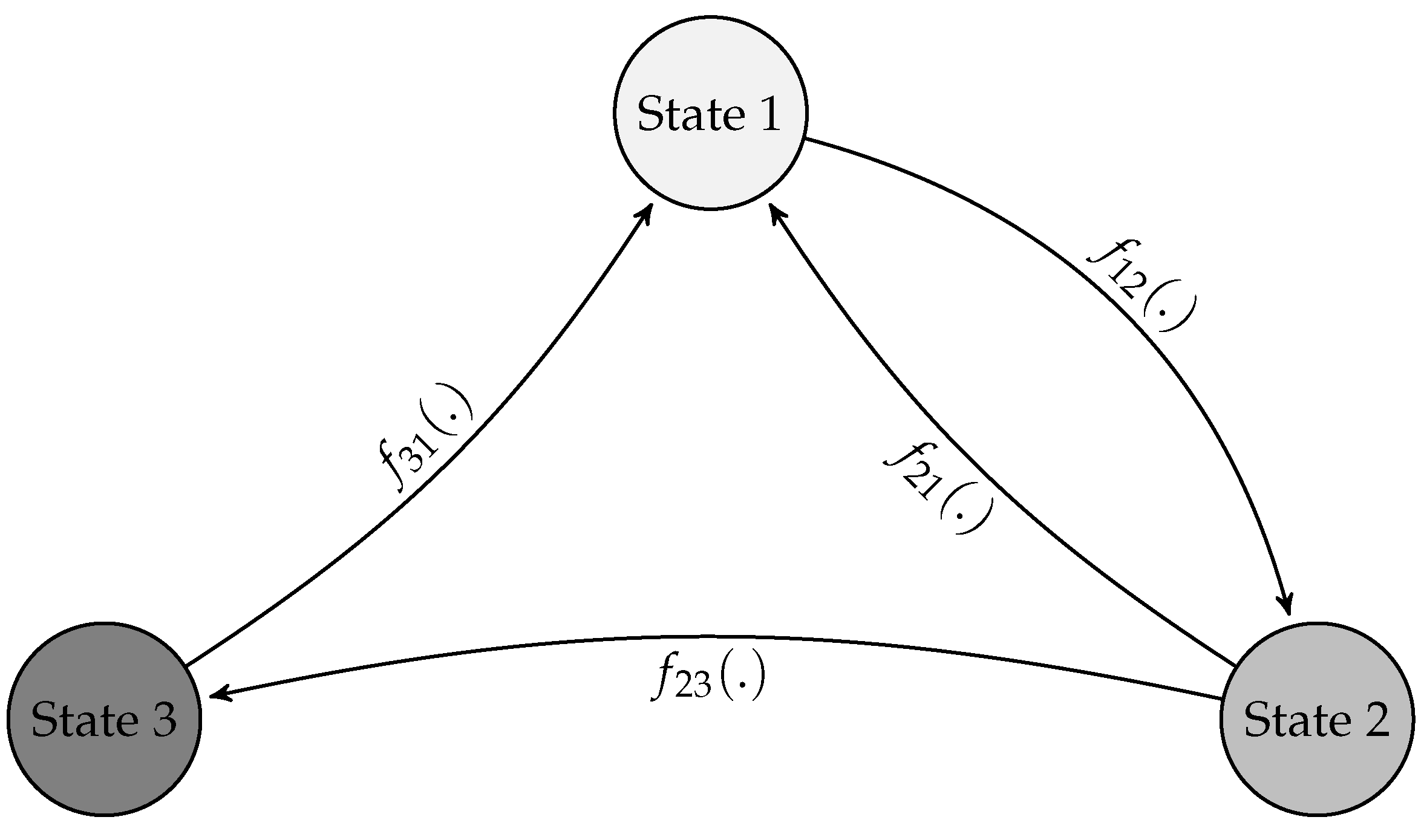
In this section, we will present a numerical example considering a semi-Markov model that governs a repairable system. The setting is as follows: the state space is E = { 1 , 2 , 3 } , the operational states are the first two, U = { 1 , 2 } , and the non-working state is the last one, D = { 3 } .
The transitions of the repairable semi-Markov model are given in the flowgraph of Figure 1.
The transition matrix p of the EMC J and the initial distribution μ are given by
p = 0 1 0 0.8 0 0.2 1 0 0 , μ = ( 1 ,   0 ,   0 ) .
Now, let X i j be the conditional sojourn time of the SMC Z in state i given that the next state is j ( j i ). The conditional sojourn times are given as follows:
X 12   Geometric ( 0.2 ) , X 21   discrete Weibull ( 0.8 , 1.2 ) , X 23   discrete Weibull ( 0.6 , 1.2 ) , X 31   discrete Weibull ( 0.9 , 1.2 ) ,
In the following figures, we investigate the semi-Markov repairable system in terms of the proposed reliability measures studied in Section 3.
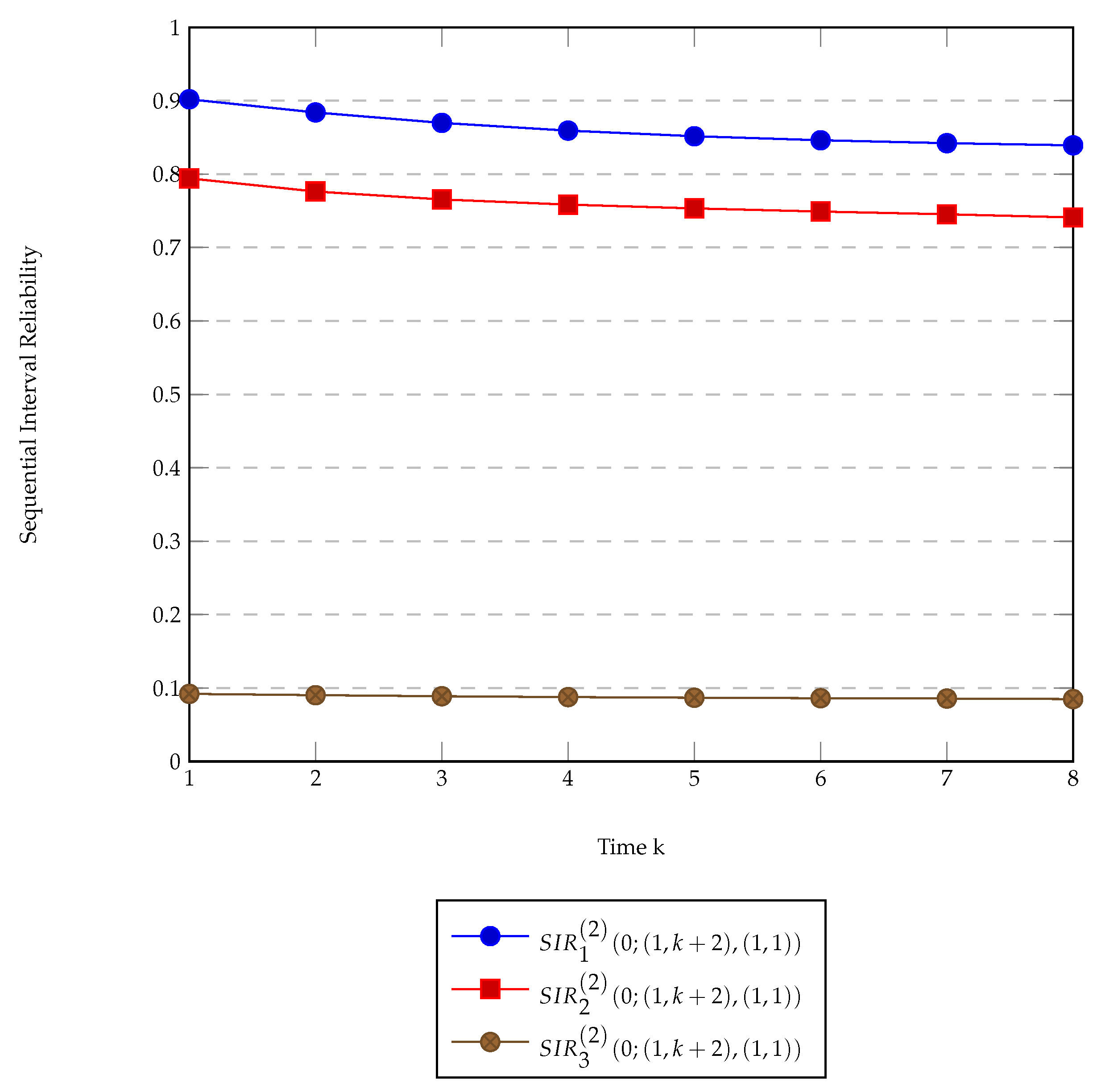
Figure 2 illustrates the conditional sequential interval reliability for two time intervals moving equally through the time with the same length (one time unit). That is the probability that the system will be operational in the time intervals ( k ,   k + 1 ) and ( k + 2 ,   k + 3 ) for k { 1 , 2 , 3 , 4 , 5 , 6 , 7 , 8 } . We have to note that, as the time k passes, then the system tends to converge to the asymptotic sequential interval reliability S I R ( 2 ) ( 0 ; t ̲ , p ̲ ) = 0.6603 , as given in Theorem 1. Furthermore, the sequential interval reliability S I R ( 2 ) ( 0 ; ( k ,   k + 2 ) , ( 1 ,   1 ) ) is equal to the conditional one S I R 1 ( 2 ) ( 0 ; ( k ,   k + 2 ) , ( 1 ,   1 ) ) due to the fact that the only possible initial state is the first one. The point here is to study the probability of a system being operational during different time periods with the same working duration and a fixed time distance between them, equal to one time unit.
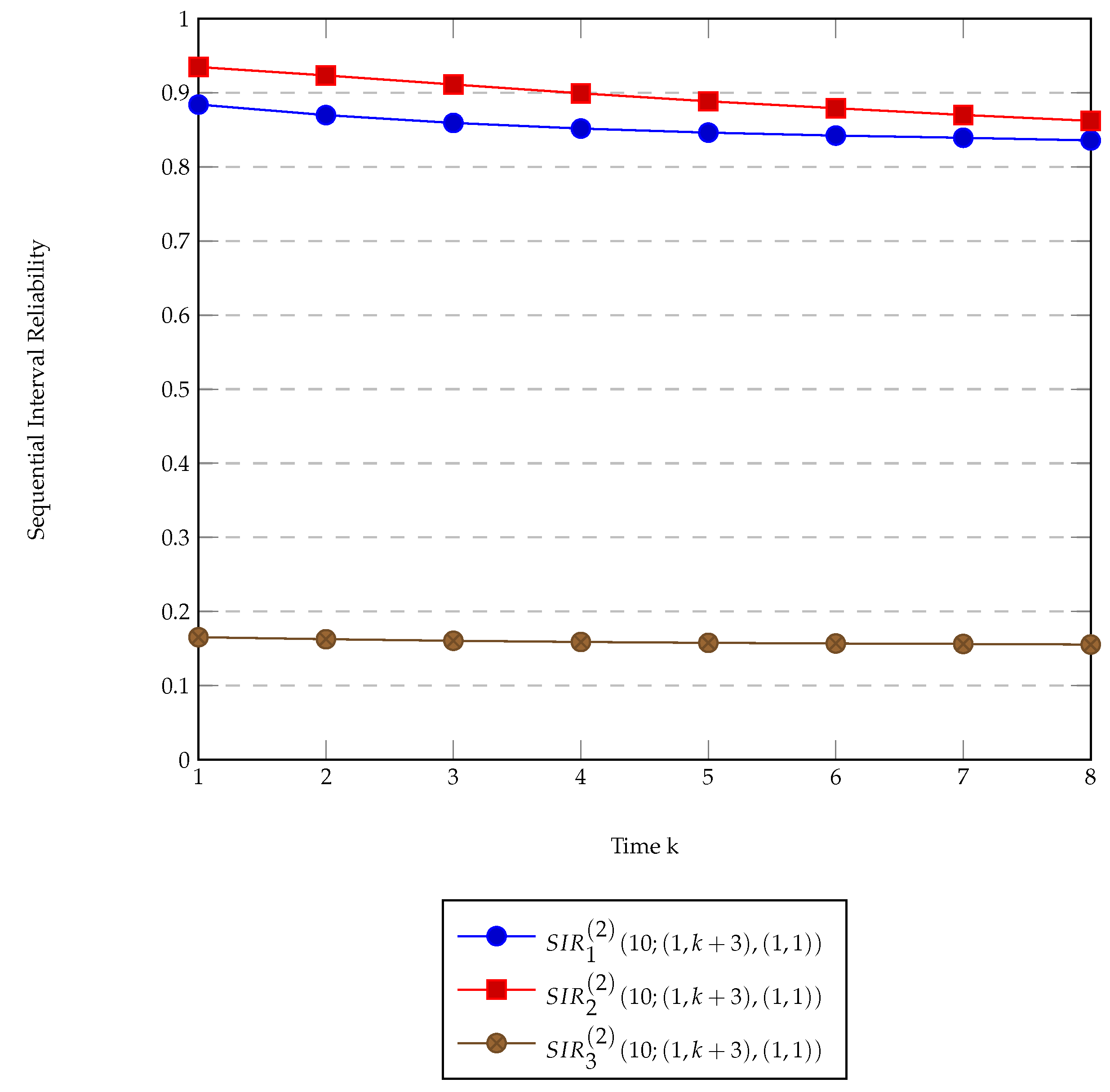
Then, Figure 3 examines the probability that the system is working during two time periods, with same working duration (equal to one time unit) and increasing the time distance between them. We considered the first interval to be fixed equal to ( 1 , 2 ) and the other moving apart with step 1 each time and be ( k + 2 , k + 3 ) for k { 1 , 2 , 3 , 4 , 5 , 6 , 7 , 8 } . It can be easily seen that the probability of the system will be still working in both time intervals and is a decreasing function of time k , which means that the two time intervals are far enough apart for the system to be operational. Note that the probability of the system starting from the non-working state 3 to be in the up-states is sufficiently small.
As in all the previous cases, the concept of the initial backward did not play a role in the simulations (Figure 2 and Figure 3), and in Figure 4, the sequential interval reliability with the initial backward v = 10 is examined. The first time interval is considered as fixed, ( 1 , 2 ) , and the other one is moving apart with step 1 each time and it is ( k + 3 ,   k + 4 ) for k { 1 , 2 , 3 , 4 , 5 , 6 , 7 , 8 } .
From the point of view of real applications, the proposed reliability measures can be applied to a huge variety of physical phenomena which they characterised from time dependence. In the literature, a lot of research works are presented for modelling a variety of such phenomena via semi-Markov processes, from financial [23] to power demand [29]. D’Amico et al. ([23,26]) proposed a semi-Markov model and associated reliability measures for constructing a credit risk model that solves problems arising from the non-Markovianity nature of the phenomenon. Further developments and recent contributions on this aspect are provided in [28,30,31].
The characteristics of semi-Markov chains which allow for no-memoryless sojourn time distributions, permit considering the duration problem in an effective way. Indeed, it is possible to define and compute different probabilities of changing state, default probabilities included, taking into account the permanence of time in a rating class. This aspect is crucial in credit rating studies because the duration dependence of transition probabilities naturally translates in many financial indicators, which change their values according to the time elapsed in the last rating class, see, e.g., [32].
In the case of financial modelling (see, e.g., [33]), the presented results could be applied in order to create advanced credit scoring models. A financial asset, similarly to government bond, usually takes a “grade” based on the reliability of the country to pay the debt (also known as creditworthiness). These grades strongly affect the interest rates of the country’s debt and they are clearly separated. Let us consider the following set of states, from a simple point of view, as the ratings:
E = { A , B , C } .
If the country bond receives a rating in the set U = { A , B } , this means that it is thought to be creditworthy and can borrow money from the markets with reasonable interest rates. On the contrary, if the rating is within the set D = { C } , then the country cannot borrow money from the markets due to very high interest rates caused from its problems for repaying the debt. D’Amico et al. [23] proposed flexible reliability measures based on semi-Markov processes for constructing a credit risk model that solves the problems arising from the non-Markovianity nature of the phenomenon. Following that work, the measures proposed in the present paper can be applied in the same way as follows:
  • The conditional sequential interval reliability with final backward S I R k ( N ) ( v ;   t ̲ ,   p ̲ ) gives the probability that the bond remains creditworthy in a sequence of different time intervals { [ t i , t i + p i ] } i = 1 ,   ,   N given its current rating and assuming a secondary process B t . This measure allows us to estimate the credit risk of the asset for different time periods and at the same time by knowing the complete trajectory of the system due to the backward process B t .
  • The sequential interval reliability S I R ( N ) ( v ;   t ̲ ,   p ̲ ) which gives the probability that the bond remains creditworthy in a sequence of different time intervals { [ t i , t i + p i ] } i = 1 ,   ,   N without taking into account the current rating. To implement this measure, we have to know the initial probability of the system being in each state.
It became clear that these measures have applications in a variety of stochastic phenomena due to their flexibility and their ability to significantly extend our knowledge about the process evolution. They can solve problems and provide answers for systems that can shift from failure to operational states, from a probabilistic point of view. Finally, they can be considered as generalisations of the classical measures of reliability for semi-Markov processes.

5. Concluding Remarks

This paper presents a new reliability indicator, called sequential interval reliability (SIR), which is evaluated for a discrete-time homogeneous semi-Markov repairable system. This indicator includes as particular cases several functions that are frequently used in reliability studies, such as the reliability and availability functions, as well as the interval reliability function.
The paper contains new theoretical results on both the transient and the asymptotic cases. More precisely, a recurrent-type equation is established for the calculation of the SIR function in the transient case and a limit theorem establishes its asymptotic behaviour. These results generalise corresponding known results for standard reliability indicators. The possibility to apply our results to real systems is shown by implementing a numerical example where the theoretical results are illustrated from a practical point of view. The paper leaves unresolved several aspects among which an important role is played by the application of the proposed indicator in different applied problems involving the use of real data.

Author Contributions

Conceptualization, G.D.; data curation, T.G.; formal analysis, V.S.B. and G.D.; methodology, G.D.; software, V.S.B. and T.G.; supervision, V.S.B.; validation, V.S.B. and T.G.; writing–original draft, V.S.B. and T.G. All authors have read and agreed to the published version of the manuscript.

Funding

Guglielmo D’Amico acknowledges the financial support by the University G. d’Annunzio of Chieti-Pescara, Italy (FAR2020).

Institutional Review Board Statement

Not applicable.

Informed Consent Statement

Not applicable.

Data Availability Statement

Not applicable.

Acknowledgments

The authors would like to express their gratitude to Professors Panagiotis-Christos Vassiliou and Andreas C. Georgiou for the opportunity to submit the present manuscript to the Special Issue Markov and Semi-Markov Chains, Processes, Systems and Emerging Related Fields for possible publication. The authors also wish to express their appreciation to the anonymous referees as well as to the editorial assistance of Devin Zhang for the time dedicated to our paper and for the valuable suggestions and constructive comments that improved both the quality and the presentation of the manuscript.

Conflicts of Interest

The authors declare no conflict of interest.

References

  1. Barbu, V.S.; Limnios, N. Semi-Markov Chains and Hidden Semi-Markov Models toward Applications—Their Use in Reliability and DNA Analysis; Lecture Notes in Statistics; Springer: New York, NY, USA, 2008; Volume 191. [Google Scholar]
  2. Janssen, J.; Manca, R. Applied Semi-Markov Processes; Springer: New York, NY, USA, 2006. [Google Scholar]
  3. Limnios, N.; Oprisan, G. Semi-Markov Processes and Reliability; Birkhäuser: Boston, UK, 2001. [Google Scholar]
  4. McClean, S. Semi-Markov models for manpower planning. In Semi-Markov Models; Janssen, J., Ed.; Springer: Berlin/Heidelberg, Germany, 1986; pp. 283–300. [Google Scholar]
  5. Papadopoulou, A.; Vassiliou, P.-C.G. Asymptotic behaviour of nonhomogeneous semi-Markov systems. Linear Algebra Its Appl. 1994, 210, 153–198. [Google Scholar] [CrossRef] [Green Version]
  6. Silvestrov, D.; Silvestrov, S. Nonlinearly Perturbed Semi-Markov Processes; Springer: Berlin/Heidelberg, Germany, 2017. [Google Scholar]
  7. Barbu, V.S.; Boussemart, M.; Limnios, N. Discrete-time semi-Markov model for reliability and survival analysis. Commun. Stat. Theory Methods 2004, 33, 2833–2868. [Google Scholar] [CrossRef]
  8. Barbu, V.S.; Limnios, N. Discrete time semi-Markov processes for reliability and survival analysis—A nonparametric estimation approach. In Parametric and Semiparametric Models with Applications to Reliability, Survival Analysis and Quality of Life; Balakrishnan, N., Nikulin, M., Mesbah, M., Limnios, N., Eds.; Birkhäuser: Basel, Switzerland, 2004; pp. 487–502. [Google Scholar]
  9. D’Amico, G. Single-use reliability computation of a semi-Markovian system. Appl. Math. 2014, 59, 571–588. [Google Scholar] [CrossRef] [Green Version]
  10. Trevezas, S.; Limnios, N. Exact MLE and asymptotic properties for nonparametric semi-Markov models. J. Nonparametr. Stat. 2011, 23, 719–739. [Google Scholar] [CrossRef] [Green Version]
  11. Limnios, N. Dependability analysis of semi-Markov systems. Reliab. Eng. Syst. Saf. 1997, 55, 203–207. [Google Scholar] [CrossRef]
  12. Limnios, N.; Ouhbi, B. Nonparametric estimation of some important indicators in reliability for semi-Markov processes. Stat. Methodol. 2006, 3, 341–350. [Google Scholar] [CrossRef]
  13. Ouhbi, B.; Limnios, N. Nonparametric reliability estimation of semi-Markov processes. J. Stat. Plan. Inference 2003, 109, 155–165. [Google Scholar] [CrossRef]
  14. Votsi, I.; Gayraud, G.; Barbu, V.S.; Limnios, N. Hypotheses testing and posterior concentration rates for semi-Markov processes. In Statistical Inference for Stochastic Processes; Springer: Berlin/Heidelberg, Germany, 2021. [Google Scholar]
  15. Wang, Y.; Shahidehpour, M.; Guo, C. Applications of survival functions to continuous semi-Markov processes for measuring reliability of power transformers. J. Mod. Power Syst. Clean Energy 2017, 5, 959–969. [Google Scholar] [CrossRef]
  16. Blasi, A.; Janssen, J.; Manca, R. Numerical treatment of homogeneous and non-homogeneous semi-Markov reliability models. Commun. Stat. Theory Methods 2004, 33, 697–714. [Google Scholar] [CrossRef]
  17. Corradi, G.; Janssen, J.; Manca, R. Numerical treatment of homogeneous semi-Markov processes in transient case—A straightforward approach. Methodol. Comput. Appl. Probab. 2004, 6, 233–246. [Google Scholar] [CrossRef]
  18. Moura, M.D.C.; Droguett, E.L. Mathematical formulation and numerical treatment based on transition frequency densities and quadrature methods for non-homogeneous semi-Markov processes. Reliab. Eng. Syst. Saf. 2009, 94, 342–349. [Google Scholar] [CrossRef]
  19. Wu, B.; Maya, B.I.G.; Limnios, N. Using semi-Markov chains to solve semi-Markov processes. In Methodology and Computing in Applied Probability; Springer: Berlin/Heidelberg, Germany, 2020. [Google Scholar]
  20. Georgiadis, S.; Limnios, N. Interval reliability for semi-Markov systems in discrete time. J. Soc. Fr. Stat. 2014, 153, 152–166. [Google Scholar]
  21. D’Amico, G.; Manca, R.; Petroni, F.; Selvamuthu, D. On the computation of some interval reliability indicators for semi-Markov systems. Mathematics 2021, 9, 575. [Google Scholar] [CrossRef]
  22. Georgiadis, S.; Limnios, N. Nonparametric estimation of interval reliability for discrete-time semi-Markov systems. J. Stat. Theory Pr. 2015, 10, 20–39. [Google Scholar] [CrossRef] [Green Version]
  23. D’Amico, G.; Janssen, J.; Manca, R. Initial and final backward and forward discrete time non-homogeneous semi-Markov credit risk models. Methodol. Comput. Appl. Probab. 2010, 12, 215–225. [Google Scholar] [CrossRef]
  24. Csenki, A. On the interval reliability of systems modelled by finite semi-Markov processes. Microelectron. Reliab. 1994, 34, 1319–1335. [Google Scholar] [CrossRef]
  25. Csenki, A. An integral equation approach to the interval reliability of systems modelled by finite semi-Markov processes. Reliab. Eng. Syst. Saf. 1995, 47, 37–45. [Google Scholar] [CrossRef]
  26. D’Amico, G.; Jacques, J.; Manca, R. Homogeneous semi-Markov reliability models for credit risk management. Decis. Econ. Financ. 2005, 28, 79–93. [Google Scholar] [CrossRef]
  27. Howard, R. Dynamic Probabilistic Systems; Wiley: New York, NY, USA, 1971; Volume 2. [Google Scholar]
  28. Vassiliou, P.-C.G. Non-homogeneous semi-Markov and Markov renewal processes and change of measure in credit risk. Mathematics 2021, 9, 55. [Google Scholar] [CrossRef]
  29. Perman, M.; Senegacnik, A.; Tuma, M. Semi-Markov models with an application to power-plant reliability analysis. IEEE Trans. Reliab. 1997, 46, 526–532. [Google Scholar] [CrossRef]
  30. Vasileiou, A.; Vassiliou, P.-C.G. An inhomogeneous semi-Markov model for the term structure of credit risk spreads. Adv. Appl. Probab. 2006, 38, 171–198. [Google Scholar] [CrossRef]
  31. Vassiliou, P.-C.G. Semi-Markov migration process in a stochastic market in credit risk. Linear Algebra Its Appl. 2014, 450, 13–43. [Google Scholar] [CrossRef]
  32. D’Amico, G.; Janssen, J.; Manca, R. Downward migration credit risk problem: A non-homogeneous backward semi-Markov reliability approach. J. Oper. Res. Soc. 2016, 67, 393–401. [Google Scholar] [CrossRef]
  33. Bulla, J.; Bulla, I. Stylized facts of financial time series and hidden semi-Markov models. Comput. Stat. Data Anal. 2006, 51, 2192–2209. [Google Scholar] [CrossRef] [Green Version]
Figure 1. Semi-Markov model.
Mathematics 09 01997 g001
Figure 2. Sequential interval reliability plot with equally moving intervals.
Mathematics 09 01997 g002
Figure 3. Sequential interval reliability plot with intervals moving apart.
Mathematics 09 01997 g003
Figure 4. Sequential interval reliability plot with the initial backward ( v = 10 ) and intervals moving apart.
Mathematics 09 01997 g004
Publisher’s Note: MDPI stays neutral with regard to jurisdictional claims in published maps and institutional affiliations.

