Abstract
In this paper, we are interested in the study of a Caputo time fractional advection–diffusion equation with nonhomogeneous boundary conditions of integral types and . The existence and uniqueness of the given problem’s solution is proved using the method of the energy inequalities known as the “a priori estimate” method relying on the range density of the operator generated by the considered problem. The approximate solution for this problem with these new kinds of boundary conditions is established by using a combination of the finite difference method and the numerical integration. Finally, we give some numerical tests to illustrate the usefulness of the obtained results.
1. Introduction
Fractional Partial Differential Equations (FPDEs) have become very important in recent years due to their use in several mathematical models. FPDEs are considered as the generalization of a partial differential equation (PDE) of an integer order of an arbitrary order. These generalizations play an essential role in engineering, physics and applied mathematics. Due to the properties of Fractional Differential Equations , different models are created for complex phenomena using FPDEs, for example, in electroanalytical chemistry, viscoelasticity [1,2], porous environment, fluid flow, thermodynamic [3,4], diffusion transport, rheology [5,6,7], electromagnetism, signal processing [8], electrical network [9] and others [10,11,12]. Some relevant applications of fractional differential equations in the modeling of tribo-fatigue systems and new materials can be mentioned as methods for the experimental study of friction in an active system [13], the volumetric damage state of the tribofatigue system in [14], the tribo-fatigue damage transition and mapping for wheel material under rolling–sliding contact condition [15]; this study is based on construction of a tribo-fatigue damage map of high-speed railway wheel material under different tangential forces and contact pressure conditions through JD-1 testing equipment. Several problems have been mentioned in modern physics and technology using partial differential equations where the nonlocal conditions are described by integrals as and . These integral conditions are of great interest due to their applications in many fields: In population dynamics, heat diffusion–advection, models of blood circulation, chemical engineering thermoelasticity [16]. The existence and uniqueness of the solution of these problems have been studied by many authors [17,18,19,20]. Some results have been obtained by construction of a variational formulation which depends on the choice of spaces and their norms, Lax–Milgram theorem, Poincaré theorem, fixed point theory and Laplace transforms. For the numerical study of FPDE with classical boundary nonlocal conditions, we can cite the works of A. Alikhanov [21,22,23], Meerschaert, M.M, S. Shen and F Liu [24,25], El-Nabulsi, R.A [26,27,28] and others [29,30,31,32,33]. Among these authors we can cite Yuriy Povstenko [34] who studied the time fractional diffusion-wave equation with classic boundary conditions. Taki and Bouziani [35] have studied a problem of FPDE which has the boundary condition of integral type with respect to time derivative of order In this paper, we are interested in a new problem of FPDE with two boundary conditions of integrals types; and . We consider the time fractional advection–diffusion equation, obtained by replacing the second-order time derivative in standard wave equation with a fractional derivative of order and classical boundary conditions with integral boundary conditions. The physical interpretation of the fractional derivative is that it represents a degree of memory in the diffusing material. For the theoretical study, we use the energy inequalities method to prove the existence and the uniqueness. The numerical study is based on the application of a combination of the finite difference method with a numerical integration method to obtain an approximate solution of the proposed problem. We use a uniform space–time discretization. The Caputo fractional operator of order is approximated by a scheme called , and the integer-order differential operators are approximated by central and advanced numerical schemes. Stability and convergence of the numerical scheme obtained show that the method used is conditionally stable and convergent. Numerical tests carried out give very satisfactory results; that is, the values of the approximate solution are very close to the exact solution. All numerical and graphical results obtained are produced using MATLAB software.
2. Notions and Preliminaries
First we need a definition of Caputo derivative to explain the problem that we shall study in this work: Let denote the gamma function. For any positive non-integer value the Caputo derivative is defined as follows:
Definition 1
(See [17]). Let us denote by the space of continuous functions with compact support in and its bilinear form is given by
where
For , we have and The bilinear form (1) is considered as scalar product on when it is not complete.
Definition 2
(See [18]). We denote by
the completion of for the scalar product defined by (1).The norm associated to the scalar product is
Lemma 1
(See [12]). For all we obtain
Definition 3
(See [12]). Let X be a Banach space with the norm , and let u: be an abstract function; by we denote the norm of the element at a fixed t.
We denote by the set of all measurable abstract functions from into X such that
Lemma 2.
(Cauchy inequality with ε) (See [12]). For all and arbitrary variables a,b we have the following inequality:
Definition 4
(See [2]). The left Caputo derivative for can be expressed as
Definition 5
(See [2]). The integral of order α of the function is defined by:
Lemma 3
(See [12]). For all real we have the inequality
Lemma 4
(See [35]). For all real we have the inequality
3. Theoretical Study
In this section, we prove the existence and uniqueness of the strong solution and its dependence on the data of the problem of fractional partial differential equations (FPDEs) with boundary conditions of integral type.
3.1. Position of the Problem
In the rectangular domain
we consider the fractional differential equation:
With Equation (4), we associate the initial conditions:
and the purely integral conditions
where et g are known continuous functions.
Hypothesis 1.
(1) For all , we assume that
(2) For all there exist and such that
this hypothesis is equivalent to the following one.
There exists such that: Every positive number could be written as with and ε
(3) The functions and satisfy the following compatibility conditions
Our proof consists of three essential steps:
- Reformulation of the problem into a problem with homogeneous conditions.
- The uniqueness of the solution to the problem using the a priori estimate method.
- The existence of the solution of the problem based on the density of the range of the operator generated by the abstract formulation of the problem.
3.2. Reformulation of the Problem
We transform a problem ((4)–(6)) with nonhomogeneous integral conditions to the equivalent problem with homogeneous integral conditions by introducing a new unknown function defined by
where
Now we study a new problem with homogeneous integral conditions
where
and
Thus, instead of seeking for solution v of problems (4)–(6), we establish the existence and the uniqueness of the solution u of problem (15)
The solution v is simply given by:
3.3. Energy Inequality Method and Consequences
To prove the existence of the solution, we use the energy inequality method known also as the “a priori estimate” method, which consists mainly of reformulating problem (15) in an equivalent operational form:
where the operator acts from B to F, where B is a Banach space of functions with the finite norm:
and F is a Hilbert space consisting of all the elements with the finite norm:
Let the domain of the operator be the set of all functions u such that and u satisfy the integral conditions (6).
Theorem 1.
We proved the uniqueness of the solution in the case of existence, and we have
Corollary 1.
The operator L from B to F has a closure .
Proof.
See [18]. □
The a priori estimate (19) can be extended to cover the strong solution of problem (15) by passing to the limit.
Corollary 2.
The range of the operator is closed in F and
Consequently, the strong solution of the problem is unique if it exists, and depends continuously on
3.4. Existence of the Solution
To prove the existence, it suffices to prove that is dense in F; that is, its orthogonal is reduced to the singleton
Theorem 2.
Let us suppose that assumptions (7) and (8) and integral conditions (6) are filled, and for and for all , we have
then ω is almost everywhere in
Proof.
We can rewrite Equation (30) as follows
We express the function in terms of u as follows:
Substituting by its representation (32) into (31), integrating by parts and taking into account conditions (6) and assumptions (7) and (8), we obtain:
□
Using condition (6) under assumptions, we find
By Lemmas 2–4 we obtain
Then
We obtain
So in which gives in
4. Numerical Study
In this section we present the numerical technique that we will apply to the problem considered above, and we illustrate the schemes obtained with well-chosen applications.
4.1. Finite Difference Method
4.1.1. Discretization of the Problem
We consider a uniform subdivision of intervals and as follows
We denote by the approximate solution of at point , and L the operator defined by
where
From the Taylor development of function v at the point we have
The discretization of Caputo derivative fractional operator [25] with is defined by
Writing fractional differential Equation (4) in point , we find
Then
where
To eliminate , we use initial condition (5); we find
Therefore,
For relation (41) gives
By conditions (6), and the trapeze method we obtain,
For
For
Matrix’s form
We denote by
To solve the system (45) we can apply one of the direct methods.
4.1.2. General Case
It is readily seen that, for
where
Lemma 5.
If the numerical scheme (41) is equivalent to
Proof.
From scheme (41), we have
□
So
Using conditions (6), and by trapeze method we obtain,
For
For
Matrix’s form
We take expression (49) for and Equations (50) and (51) to formulate the matrix systems:
where
is square matrix defined by
and
In order to prove system (52) has a unique solution we denote as an eigenvalue of the matrix , and is a nonzero eigenvector corresponding to
We choose i such that
Then
Therefore
Substituting the values of into (53), and taking into account that , are negative and we get:
For
For
For
From the above we conclude for
If then
If and then all eigenvalues of matrix are strictly positive; therefore, is invertible.
4.2. Stability and Convergence
4.2.1. Stability
We have
Let be the approximate solution of (49), and the error at point defined by
For we apply (42) and we get
So
Therefore the method is stable.
Lemma 6.
For the scheme (48) is stable and we have
Proof.
We use mathematical induction. □
We assume and where
Then
Therefore, the method is stable.
4.2.2. Convergence
Let be the exact solution and be the approximate solution of scheme (38); we put for .
Then
So
Hence
Taking
for , we get
We have
Hence
We assume: ; .
From (60), we get
We have
Hence
Therefore, the method is convergent.
4.3. Applications
In this section, we give some numerical investigation tests.
The analytical solution is given by
The approximate solution where A.E is the absolute error.
We see in Figure 1, Figure 2 and Figure 3 and Table 1, Table 2 and Table 3 that the absolute error(A.E) gradually decreases when the step takes small values and getting very close to zero. That is, for , , and the absolute error(A.E) decreases towards zero and the approximate solution tends towards the exact solution with the convergence order of
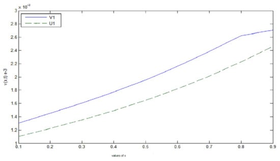
Figure 1.
.
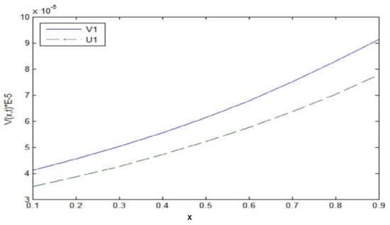
Figure 2.
.
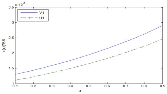
Figure 3.
.

Table 1.
.
Table 2.
, .
Table 3.
.
For (second iteration),
Table 4 shows the absolute error decrease to zero and Figure 4, Figure 5 and Figure 6 show the approximate solution after two steps tend towards the exact solution when close to zero, with convergence order
Table 4.
.
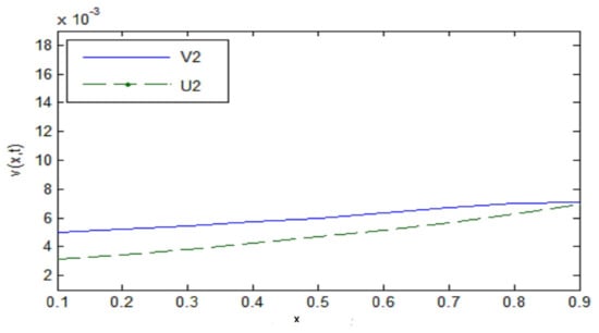
Figure 4.
.
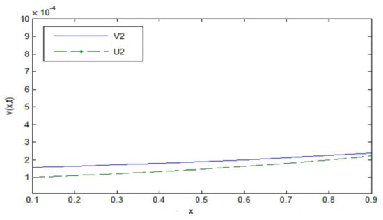
Figure 5.
.
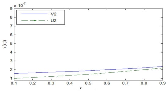
Figure 6.
.
Remark 1.
For space step we find Figure A1 and Figure A2 in Appendix A.
Example 2.
We take:
The analytical solution of this problem is given by
Table 5.
.
Table 6.
.
Table 7.
, .
In this example from Table 5, Table 6 and Table 7 and Figure 7, Figure 8 and Figure 9 we see again for space step the absolute error tends to zero when the time step takes a value close to zero, with convergence order In Figure 9 we take into account x to see the variation of error because it is very close to zero when x

Figure 7.
, .
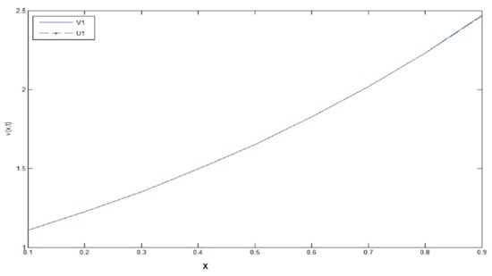
Figure 8.
, .
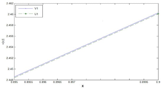
Figure 9.
, , x.
Remark 2.
For the space step we find Figure A3, Figure A4, Figure A5 in Appendix A.
Table 8 shows the error norm for different values of defined by
Table 8.
.
We see in Table 8, for the space step , and for the different values of , the error keeps the same behavior; that is, the error norm tends towards zero when the time step takes values close to zero, with an order of convergence . For (value close to 1) the error is greater compared to the case (value close to 2) due of the fractional operator being approximated by the formula called
5. Conclusions
In this paper, the existence and uniqueness of the solution of a Caputo time fractional problem with nonhomogeneous boundary integral conditions are established. We use the “energy inequality” method which is an efficient functional analysis method.
For the numerical study, these kinds of boundary conditions have been applied for the first time to such problems, where we combined the finite difference method with the numerical integration to obtain the approximate solution. The results obtained by this technique are very encouraging from the point of view that the numerical schemes are stable and convergent.
As further research directions, we aim at studying the same problem using the compact finite difference method in order to obtain more precise results, change the sense of fractional derivatives and/or extend the study to time–space fractional derivatives.
Author Contributions
Conceptualization, S.B., A.M. and A.K.; methodology, S.B. and A.M.; software, S.B.; validation, A.K.; formal analysis, A.K.; investigation, S.B. and A.K.; writing—original draft preparation, S.B.; writing—review and editing, A.K.; visualization, S.B., A.M., A.K.; supervision, A.M. and A.K. All authors have read and agreed to the published version of the manuscript.
Funding
This research received no external funding.
Institutional Review Board Statement
Not applicable.
Informed Consent Statement
Not applicable.
Data Availability Statement
Not applicable.
Conflicts of Interest
The authors declare no conflict of interest.
Appendix A
In Example 1 for
From Table A1 and Table A2 and Figure A1 and Figure A2 with space step , we see that the approximate solution tends to the exact solution when takes values close to zero, with convergence order
Table A1.
The absolute error for .
Table A1.
The absolute error for .
| 5 × 10 | 6 × 10 | 6 × 10 | 7 × 10 | 8 × 10 | 9 × 10 | 10 | 10 | 10 | 10 | 10 |
| 5 × 10 | 6 × 10 | 7 × 10 | 7 × 10 | 8 × 10 | 9 × 10 | 10 | 10 | 10 | 10 | 10 |
| 5 × 10 | 6 × 10 | 7 × 10 | 7 × 10 | 8 × 10 | 9 × 10 | 10 | 10 | 10 | 10 | 10 |
| 6 × 10 | 6 × 10 | 7 × 10 | 7 × 10 | 8 × 10 | 9 × 10 | 10 | 10 | 10 | 10 | 10 |
| 6 × 10 | 6 × 10 | 7 × 10 | 7 × 10 | 8 × 10 | 9 × 10 | 10 | 10 | 10 | 10 | 10 |
| 6 × 10 | 6 × 10 | 7 × 10 | 7 × 10 | 8 × 10 | 9 × 10 | 10 | 10 | 10 | 10 | 10 |
| 6 × 10 | 6 × 10 | 7 × 10 | 8 × 10 | 8 × 10 | 9 × 10 | 10 | 10 | 10 | 10 | 10 |
| 6 × 10 | 6 × 10 | 7 × 10 | 8 × 10 | 8 × 10 | 9 × 10 | 10 | 10 | 10 | 10 | 10 |
| 6 × 10 | 6 × 10 | 7 × 10 | 8 × 10 | 8 × 10 | 9 × 10 | 10 | 10 | 10 | 10 | 10 |
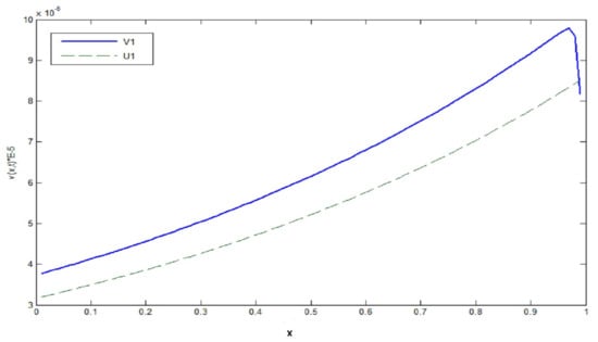
Figure A1.
.
Table A2.
The absolute error for .
Table A2.
The absolute error for .
| 5 × 10 | 6 × 10 | 6 × 10 | 7 × 10 | 8 × 10 | 8 × 10 | 9 × 10 | 10 | 10 | 10 | 10 |
| 5 × 10 | 6 × 10 | 6 × 10 | 7 × 10 | 8 × 10 | 9 × 10 | 9 × 10 | 10 | 10 | 10 | 10 |
| 5 × 10 | 6 × 10 | 6 × 10 | 7 × 10 | 8 × 10 | 9 × 10 | 9 × 10 | 10 | 10 | 10 | 10 |
| 5 × 10 | 6 × 10 | 7 × 10 | 7 × 10 | 8 × 10 | 9 × 10 | 10 | 10 | 10 | 10 | 10 |
| 5 × 10 | 6 × 10 | 7 × 10 | 7 × 10 | 8 × 10 | 9 × 10 | 10 | 10 | 10 | 10 | 10 |
| 5 × 10 | 6 × 10 | 7 × 10 | 7 × 10 | 8 × 10 | 9 × 10 | 10 | 10 | 10 | 10 | 10 |
| 6 × 10 | 6 × 10 | 7 × 10 | 7 × 10 | 8 × 10 | 9 × 10 | 10 | 10 | 10 | 10 | 10 |
| 6 × 10 | 6 × 10 | 7 × 10 | 7 × 10 | 8 × 10 | 9 × 10 | 10 | 10 | 10 | 10 | 10 |
| 6 × 10 | 6 × 10 | 7 × 10 | 8 × 10 | 8 × 10 | 9 × 10 | 10 | 10 | 10 | 10 | 10 |
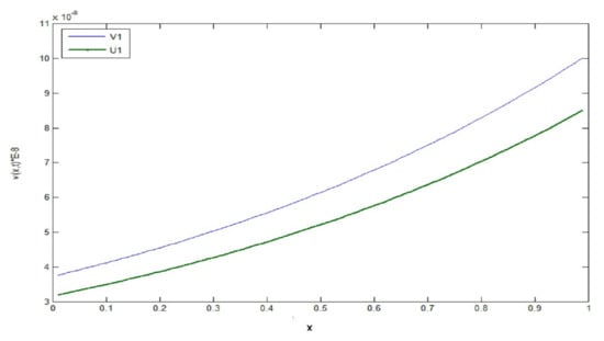
Figure A2.
.
In Example 2, for ,
The Figure A3, Figure A4, Figure A5 show where the space step is fixed at and the time step decreases towards zero , the approximate solution tends to the exact solution , in the case where we see that the two curves of and are almost identical.
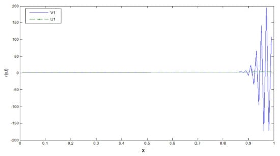
Figure A3.
.
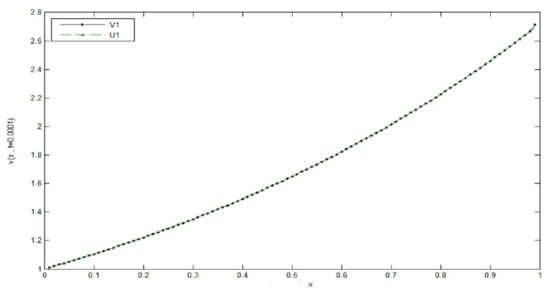
Figure A4.
.
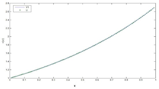
Figure A5.
.
References
- Mainardi, F. Fractional diffusive waves in viscoelastic solids. Nonlinear Waves Solids 1995, 137, 93–97. [Google Scholar]
- Podlubny, I. Fractional Differential Equations; Academic Press: San Diego, CA, USA, 1999. [Google Scholar]
- He, J.H. Approximate analytical solution for seepage flow with fractional derivatives in porous media. Comput. Methods Appl. Mech. Eng. 1998, 167, 57–68. [Google Scholar] [CrossRef]
- Kilbas, A.A.; Srivastava, H.M.; Trujillo, J.J. Theory and Applications of Fractional Differential Equations; Elsevier: Amsterdam, The Netherlands, 2006. [Google Scholar]
- Alikhanov, A.A. Boundary value problems for the di usion equation of the variable order in differential and difference settings. Appl. Math. Comput. 2012, 219, 3938–3946. [Google Scholar]
- Li, X.J.; Xu, C.J. Existence and uniqueness of the weak solution of the space-time fractional diffusion equation and a spectral method approximation. Commun. Comput. Phys. 2010, 8, 1016–1051. [Google Scholar]
- Smit, W.; de Vries, H. Rheological models containing fractional derivatives. Rheol. Acta 1970, 9, 525–534. [Google Scholar] [CrossRef]
- Monje, C.A.; Chen, Y.; Vinagre, B.M.; Xue, D.; Feliu, V. Fractional-Order Systems and Controls: Fundamentals and Applications; Springer: London, UK, 2010. [Google Scholar]
- Enacheanu, O. Fractal Modeling of Electrical Networks. Ph.D. Thesis, Joseph Fourier University, Grenoble, France, October 2008; pp. 47–53. [Google Scholar]
- Kaufmann, E.R.; Mboumi, E. Positive solutions of a boundary value problem for a nonlinear. fractional differential equation. Electron. J. Qual. Theory Differ. Equ. 2007, 3, 1–11. [Google Scholar] [CrossRef]
- Furati, K.M.; Tatar, N. An existence result for a nonlocal fractional differential problem. J. Fract. Calc. 2004, 26, 43–51. [Google Scholar]
- Mesloub, S. Existence and uniqueness results for a fractional two-times evolution problem with constraints of purely integral type. Math. Methods Appl. Sci. 2016, 39, 1558–1567. [Google Scholar] [CrossRef]
- Sosnovskii, L.A.; Komissarov, V.V.; Shcherbakov, S.S. A Method of Experimental Study of Friction in a Active System. J. Frict. Wear 2012, 33, 174–184. [Google Scholar] [CrossRef]
- Shcherbakov, S.S. State of volumetric damage of tribo-fatigue systeme. Strength Mater. 2013, 45, 171–178. [Google Scholar] [CrossRef]
- He, C.; Liu, J.; Wang, W.; Liu, Q. The Tribo-Fatigue Damage Transition and Mapping for Wheel Material under Rolling-Sliding Contact Condition. Materials 2019, 12, 4138. [Google Scholar] [CrossRef] [Green Version]
- Day, W.A. A decreasing property of solutions of parabolic equations with applications to thermoelasticity. Quart. Appl. Math. 1983, 40, 319–330. [Google Scholar] [CrossRef] [Green Version]
- Anguraj, A.; Karthikeyan, P. Existence of solutions for fractional semilinear evolution boundary value problem. Commun. Appl. Anal. 2010, 14, 505–514. [Google Scholar]
- Jesus, M.-V.; Ahcene, M. Existence, uniqueness and numerical solution of a fractional PDE with integral conditions. Nonlinear Anal. Model. Control 2019, 24, 368–386. [Google Scholar]
- Benchohra, M.; Graef, J.R.; Hamani, S. Existence results for boundary value problems with nonlinear fractional differential equations. Appl. Anal. 2008, 87, 851–863. [Google Scholar] [CrossRef]
- Daftardar-Gejji, V.; Jafari, H. Boundary value problems for fractional diffusion-wave equation. Aust. J. Math. Anal. Appl. 2006, 3, 1–8. [Google Scholar]
- Alikhanov, A.A. On the stability and convergence of nonlocal difference schemes. Differ. Equ. 2010, 46, 949–961. [Google Scholar] [CrossRef]
- Alikhanov, A.A. A new difference scheme for the time fractional diffusion equation. J. Comput. Phys. 2015, 280, 424–438. [Google Scholar] [CrossRef] [Green Version]
- Alikhanov, A.A. Stability and convergence of difference schemes for boundary value problems for the fractional-order diffusion equation. Comput. Math. Math. Phys. 2016, 56, 561–575. [Google Scholar] [CrossRef]
- Meerschaert, M.M.; Tadjeran, C. Finite difference approximations for fractional advection dispersion flow equations. J. Comput. Appl. Math. 2004, 172, 65–77. [Google Scholar] [CrossRef] [Green Version]
- Shen, S.; Liu, F. Error analysis of an explicit finite difference approximation for the space fractional diffusion. Anziam J. 2005, 46, C871–C887. [Google Scholar] [CrossRef] [Green Version]
- El-Nabulsi, R.A. Finite Two-Point Space without Quantization on Noncommutative Space from a Generalized Fractional Integral Operator. Complex Anal. Oper. Theory 2018, 12, 1609–1616. [Google Scholar] [CrossRef]
- El-Nabulsi, R.A. The fractional Boltzmann transport equation. Comput. Math. Appl. 2011, 62, 1568–1575. [Google Scholar] [CrossRef] [Green Version]
- El-Nabulsi, R.A. Nonlocal-in-time kinetic energy in nonconservative fractional systems, disordered dynamics, jerk and snap and oscillatory motions in the rotating fluid tube. Int. J. Non-Linear Mech. 2017, 93, 65. [Google Scholar] [CrossRef]
- Yan, B.H.; Yu, L.; Yang, Y.H. Study of oscillating flow in rolling motion with the fractional derivative Maxwell model. Prog. Nucl. Energy 2011, 53, 132–138. [Google Scholar] [CrossRef]
- Li, X.; Yang, X.; Zhang, Y. Error estimates of mixed finite element methods for timefractional Navier-Stokes equations. J. Sci. Comput. 2017, 70, 500–515. [Google Scholar] [CrossRef]
- Yildirim, A. Analytical approach to fractional partial differential equations in fluid mechanics by means of the homotopy perturbation method. Int. J. Numer. Methods Heat Fluid Flow 2010, 20, 186–200. [Google Scholar] [CrossRef]
- Zhou, Y.; Peng, L. On the time-fractional Navier–Stokes equations. Comput. Math. Appl. 2017, 73, 874–891. [Google Scholar] [CrossRef]
- Yu, B.; Jiang, X.Y.; Xu, H.Y. A novel compact numerical method for solving the two-dimensional non-linear fractional reaction-subdiffusion equation. Numer. Algorithms 2015, 68, 923–950. [Google Scholar] [CrossRef]
- Povstenko, Y. Linear Fractional Diffusion-Wave Equation for Scientists and Engineers; Springer: Berlin/Heidelberg, Germany, 2010. [Google Scholar]
- Oussaeif, T.-E.; Bouziani, A. Existence and uniqueness of solutions to parabolic fractional differential equations with integral conditions. Electron. J. Differ. Equ. 2014, 2014, 1–10. [Google Scholar]
Publisher’s Note: MDPI stays neutral with regard to jurisdictional claims in published maps and institutional affiliations. |
© 2021 by the authors. Licensee MDPI, Basel, Switzerland. This article is an open access article distributed under the terms and conditions of the Creative Commons Attribution (CC BY) license (https://creativecommons.org/licenses/by/4.0/).