1. Introduction
When a shallow soil stratum is highly compressible and of low bearing capacity to support the load transmitted by the superstructure, piles are principally used to transmit the loads to the underlying stiffer soil strata of a higher bearing capacity. Various precious approaches have been proposed to analyze the laterally loaded piles, including the subgrade reaction approach [
1,
2] and p-y approach [
3,
4]. In the subgrade reaction approach, the supporting soil is idealized as a series of lateral elastic springs and the relationship between lateral applied force and lateral deflection pattern of a pile is treated as linear- elastic over the depth of the pile. Moreover, the subgrade reaction modulus is obtained through fitting with relevant numerical solutions [
5,
6]. In the p-y approach the soil is conveniently simulated by a series of independent non-linear springs varying with the depth, and the soil–pile interface responses are captured by representing the soil nonlinear springs with p-y curves along the pile length. Several researchers on the piles subjected to lateral loads continued to be unabated in which the soil is considered as a continuum-based model. In these studies, different approaches such as the finite element approach [
7], boundary element approach [
8], and finite difference approach [
9], have been introduced to predict the response of laterally loaded piles. A large number of studies have examined the behaviour of the soil–pile interaction of laterally loaded piles considering that the relationship between soil lateral reaction and pile deflection is linear [
10], and the lateral load behaviour of soil is non-linear. Therefore, the development of algebraic expressions via a closed form solution is proposed in this study to predict the non-linear responses of laterally loaded piles in clay strata. The proposed analytical solution in the current study provides a better approach for structural designers to simply solve for the lateral soil reaction, displacement, shear force, and bending moment responses of laterally loaded free-head long piles embedded in homogeneous cohesive soils with a constant lateral subgrade reaction with depth. Consequently, the techniques can be easily applied in practice as an alternative approach to analyse and design laterally loaded long piles. In addition, the proposed solution incorporates the contribution of the Winkler foundation model with the linear elastic-perfect-plastic p-y soil response. The proposed analytical solution is verified by comparing the results obtained for the pile’s deflection and induced bending moment with numerical results using the finite element software ANSYS. The accuracy of the location at which the maximum bending moment occurs, and the magnitude of that maximum bending moment along the pile are further verified analytically by comparing them to those obtained from the FE analysis. In addition, a numerical example is introduced to investigate the effect of the horizontal loads on the depth of the plastic zone.
2. Problem Definition and Formulation
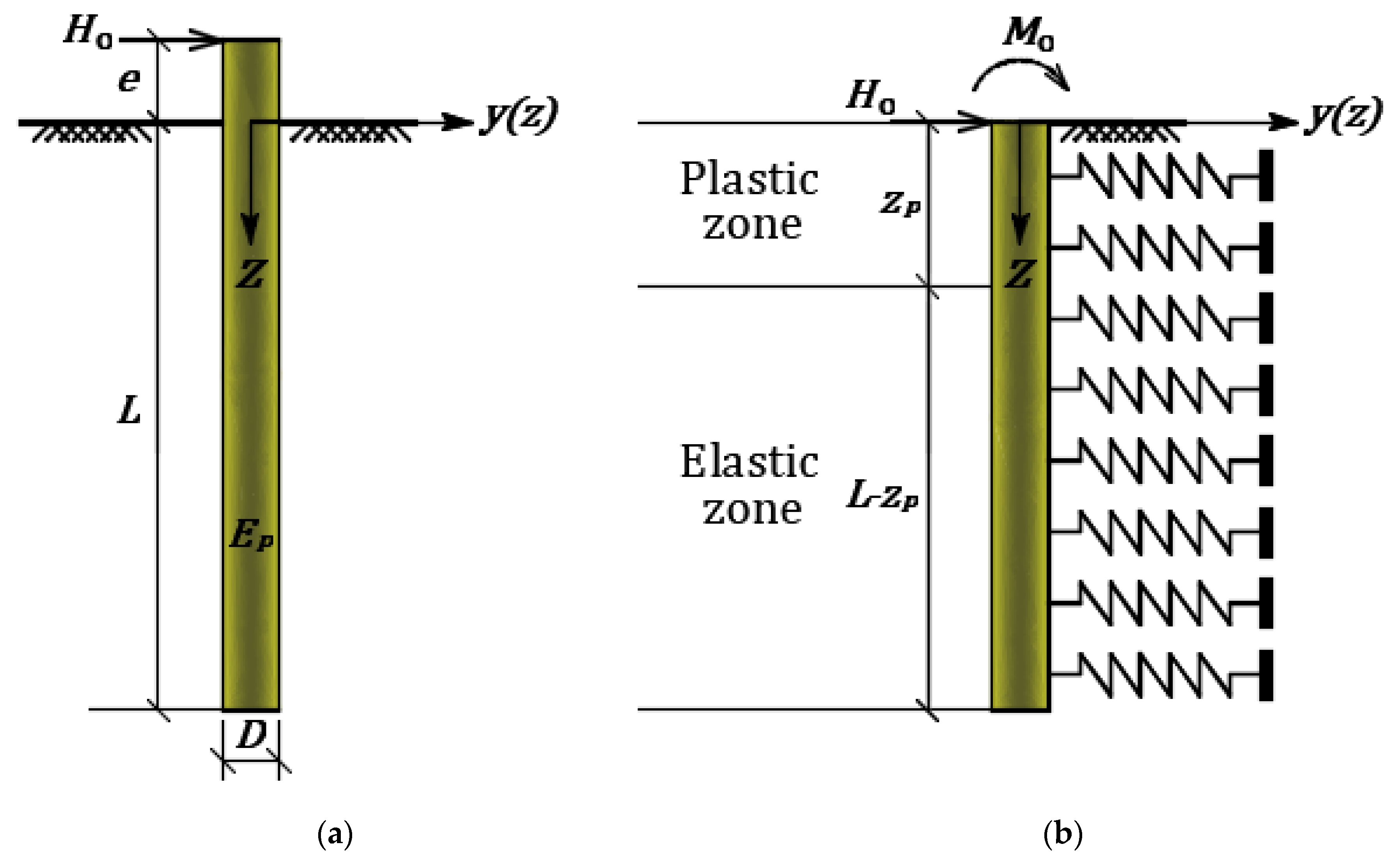
A free-head cylindrical pile of length
L, diameter
D, and Young’s modulus
embedded in a homogeneous clay soil and subjected to lateral load
at an eccentricity,
e above ground surface is schematically shown in
Figure 1a. In order to simulate the pile–soil interaction, the pile shaft is assumed to be perfectly glued to the surrounding soils suggesting that there is no relative movement along the pile–soil interface. Furthermore, a series of springs distributed along the pile shaft are used to characterize that interaction for the pile subjected to the lateral load
and bending moment,
at the ground surface, as shown in
Figure 1b.
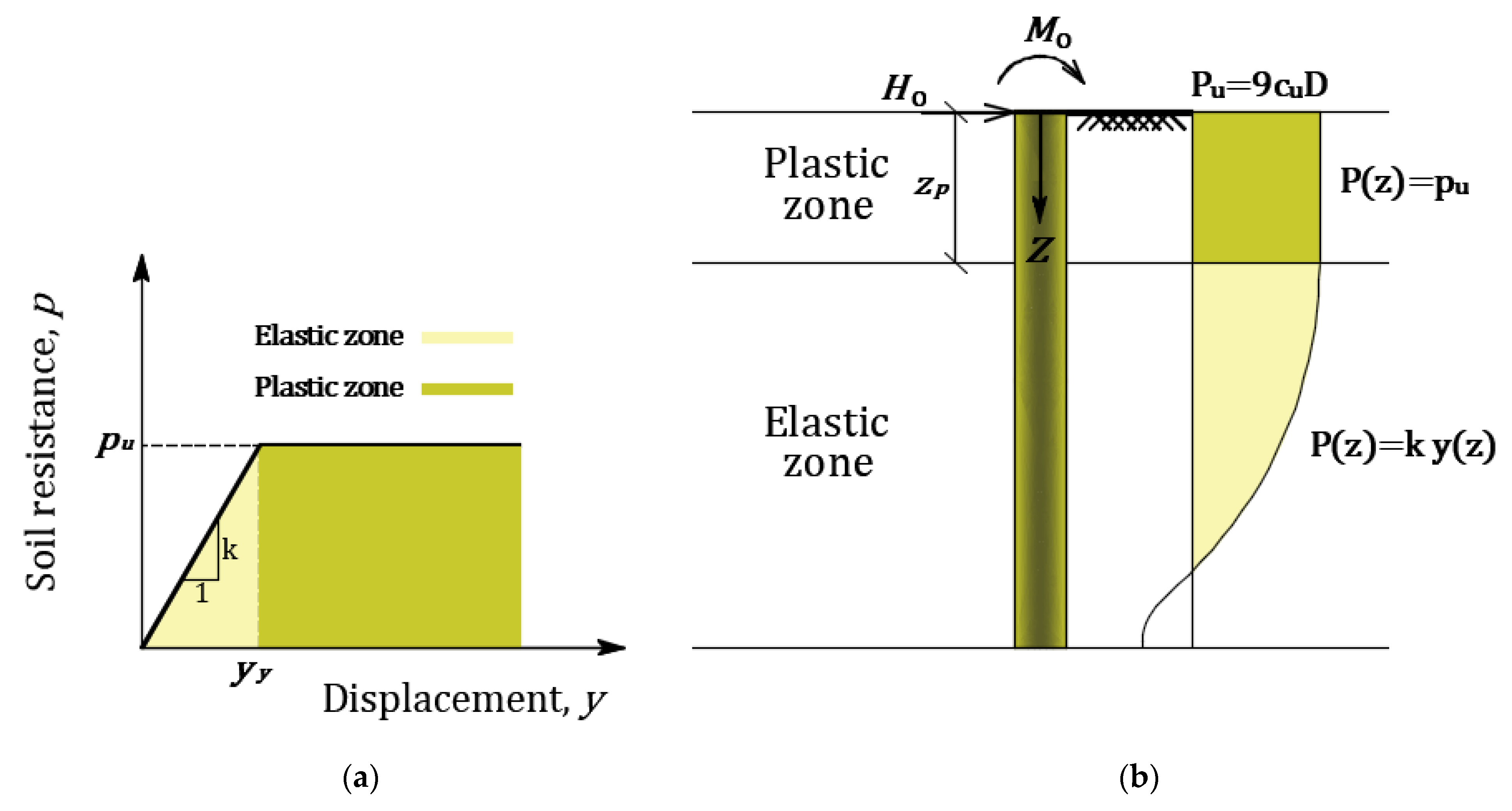
Free-head and fixed-tip boundary conditions are assumed. Therefore, the pile head is unrestrained to rotate and move laterally while the pile base is fully fixed against translation and rotation. Unquestionably, the soil behaves non-linearly under higher lateral load. This nonlinearity is described by the well-known ideal elasto-plastic p-y relationship at any depth. This model is shown in
Figure 2a in which
k is the gradient of the p-y curve that offers the soil modulus at any point
z below the surface along the pile,
is the limiting soil horizontal resistance per unit depth, and
y_
y is the threshold of soil displacement above which the soil is initiated to yield. On the other hand, the soil near the ground surface presumably yields firstly and propagates downward to a depth called plastic depth,
[
11]. Below plastic depth, the soil reaction is linear and still in the elastic state. Accordingly, the lateral soil reaction along the pile shaft may be characterized by two zones: the plastic zone above which extends to a depth
depending on both the applied lateral force and its point of application, and the bottom elastic zone below this depth (see
Figure 1b and
Figure 2b) [
12]. It is worth noting that the limiting lateral force for clay soils increases with depth from
to
at ground surface up to
to
at a depth of about 3D, and beyond this depth it keeps constant [
13]. Where
is the undrained shear strength of the soil,
D is the pile diameter. Consequently, the limiting lateral force is proposed to equal
to the end of the plastic zone (see
Figure 2b) [
14].
3. Mathematical Formulation
In the case of the pile subjected to lateral forces, it tries to push the surrounding soil horizontally in the loading direction to its limit state. Subsequently, the surface soils tend to yield, and the cracks tend to be very shallow. The lateral soil reaction along the pile shaft may be characterized by two zones: the top plastic zone which extends downward to depth
depending on both applied lateral force and its point of application, and the bottom elastic zone below this depth (see
Figure 2).
The governing flexural equation for the response of the soil–pile system according to Winkler’s foundation concept can be written as:
In the above,
E is the modulus of elasticity of concrete,
I is the effective moment of inertia,
y is the lateral deflection of the pile, and
p(
z) is the soil reaction at any point at a depth
z along the axis of the pile which may be described for the elasto-plastic model as:
where
k is the subgrade reaction modulus of the soil,
is the depth of the plastic zone, and
is the lateral limit force below which the soil reaction has a linear relationship with lateral pile deflection.
The integration of Equation (1) considering the boundary and continuity conditions presented in
Table 1 and
Table 2 leads to the analytical solution for piles subjected to lateral loads and embedded in linear-plastic soil.
3.1. Elastic Soil Behaviour
Based on the assumption that the applied lateral force does not exceed the ultimate load
, the relationship between lateral soil resistance per unit pile length and pile lateral deflection under working loads is linear–elastic. Consequently, under this assumption the governing equation of motion can be expressed as:
If one assumes that the modulus of subgrade reaction
k in clay soil is independent of depth [
15], thereby the general solution of Equation (3) is of the form:
where
β is the reciprocal of the characteristic length and
are four independent constant parameters.
Assuming that the pile is infinite and the deflection at the tip of the long piles is negligible, then the lateral deflections at working loads can be simplified as
Further higher derivatives for Equation (5) yields
By substituting Equations (5) and (9) into Equation (3),
for the free-load pile can be assigned as:
where
EI is stiffness of pile section and
D is width or diameter of pile.
Two constant parameters
are obtained for piles subjected to applied horizontal load
and applied bending moment
by imposing the equilibrium conditions for both the bending moment and shear force at pile top using
Table 1. Thereupon, by substituting the boundary conditions into Equations (7) and (8), two integration coefficients
can be determined as:
The deflection along the laterally loaded pile can be obtained by substituting Equations (11) and (12) into Equation (5) as
Consequently, the bending moment
M, and the shear force
V are found by successive differentiation of Equation (13) as:
By setting
, the point of zero shear
can be written as:
Therefore, the maximum bending moment can be obtained as follows:
3.2. Elasto-Plastic Soil Behaviour
Admittedly, the soil behavior under higher lateral load levels is predominantly non-linear. A simple approach proposed by Madhav et al. [
16] reasonably captures this nonlinearity through considering the elastic-plastic subgrade model. Consequently, the non-linear responses for long piles under lateral loading may be obtained through two zones as follows.
3.2.1. Plastic Zone
Through several integrations for Equation (18), the key responses of the pile in the plastic zone can be expressed as follows:
3.2.2. Elastic Zone
The solution of the above equations requires boundary conditions to obtain the unknown parameters
and
. All boundary conditions associated with the above equations must be determined by recourse to the boundary conditions in
Table 2. The equilibrium for the bending moment and shear force at
and compatibility for displacement and slope at
is considered.
By considering equilibrium for shear at the pile head, the undetermined constants
can be determined as:
Subsequently, by imposing the equilibrium for the bending moment at the pile head, the undetermined constants
can be expressed as:
Then, the plastic zone develops at a depth
of the form:
Applying the compatibility for slope at
by equating Equation (21) with Equation (24) yields
where
and
Similarly, applying the compatibility for deflection at
by equating Equation (22) with Equation (23) yields,
Based on Equations (21) and (22), the rotation
and horizontal deflection
of the pile at
can be expressed as
Furthermore, Equation (26) can be re-expressed as:
Applying equilibrium principles at
yields
and
is given by
There are two cases that may arise to obtain the maximum value of the bending moment and the corresponding position.
Case 1: the bending moment occurs in the elastic region.
In this case, the largest bending moment value is assumed to occur in the elastic region. Substituting into Equation (26) with
and equating with zero yields
The depth of maximum bending moment which occurs in elastic zone can be expressed as
Case 2: the bending moment occurs in the plastic region.
This case assumes the occurrence of largest bending moment value is in the plastic region. Proceeding similarly as Case 1, the depth of maximum bending moment which occurs in elastic zone can be expressed as
and its value is
4. Validation of the Proposed Methods
The capability of the proposed analytical solutions presented in this research to predict the lateral behaviour of single piles embedded in a cohesive soil and the corresponding pile responses have been demonstrated and compared with the FE results carried out using ANSYS software.
For this purpose, a concrete pile with length L = 15 m, diameter D = 0.4 m, Poisson’s ratio ν = 0.2, and Young’s modulus of elasticity Ep = 35,000 MPa is embedded in a clay layer with lateral reaction modulus ks = 50,000 kpa and shear strength Cu = 14.4 kpa. The pile head is unrestrained to rotate and move laterally while the pile tip is completely fixed.
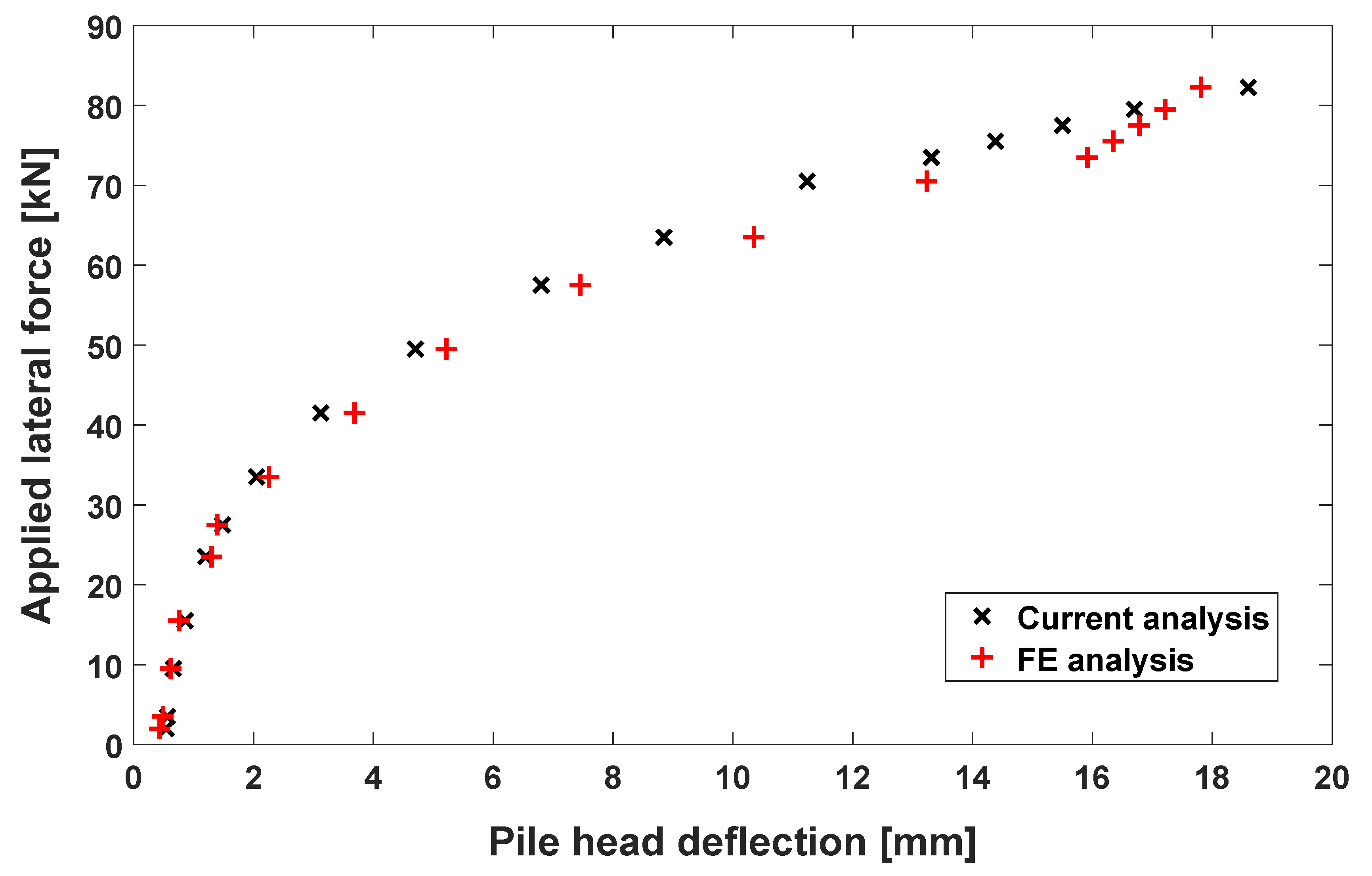
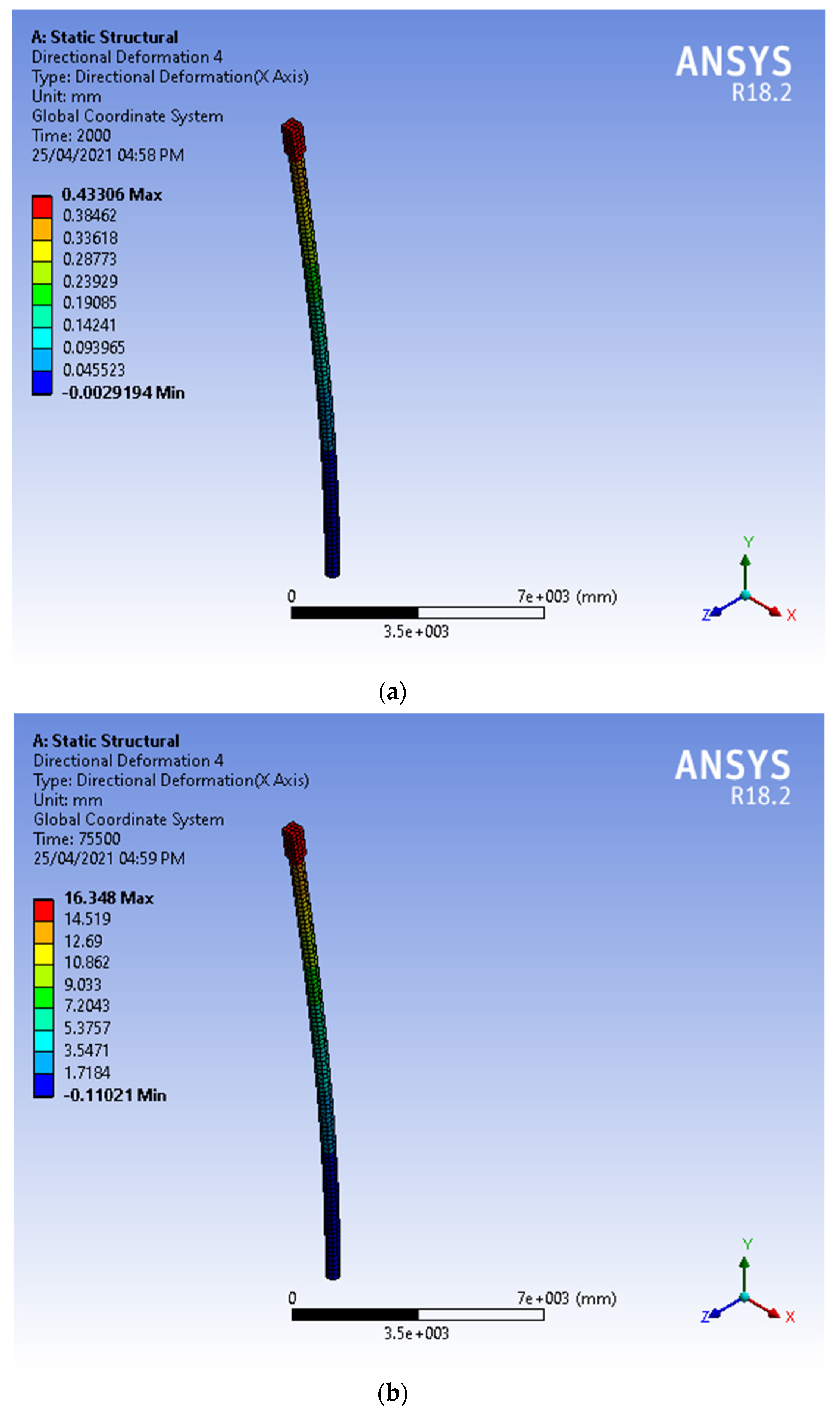
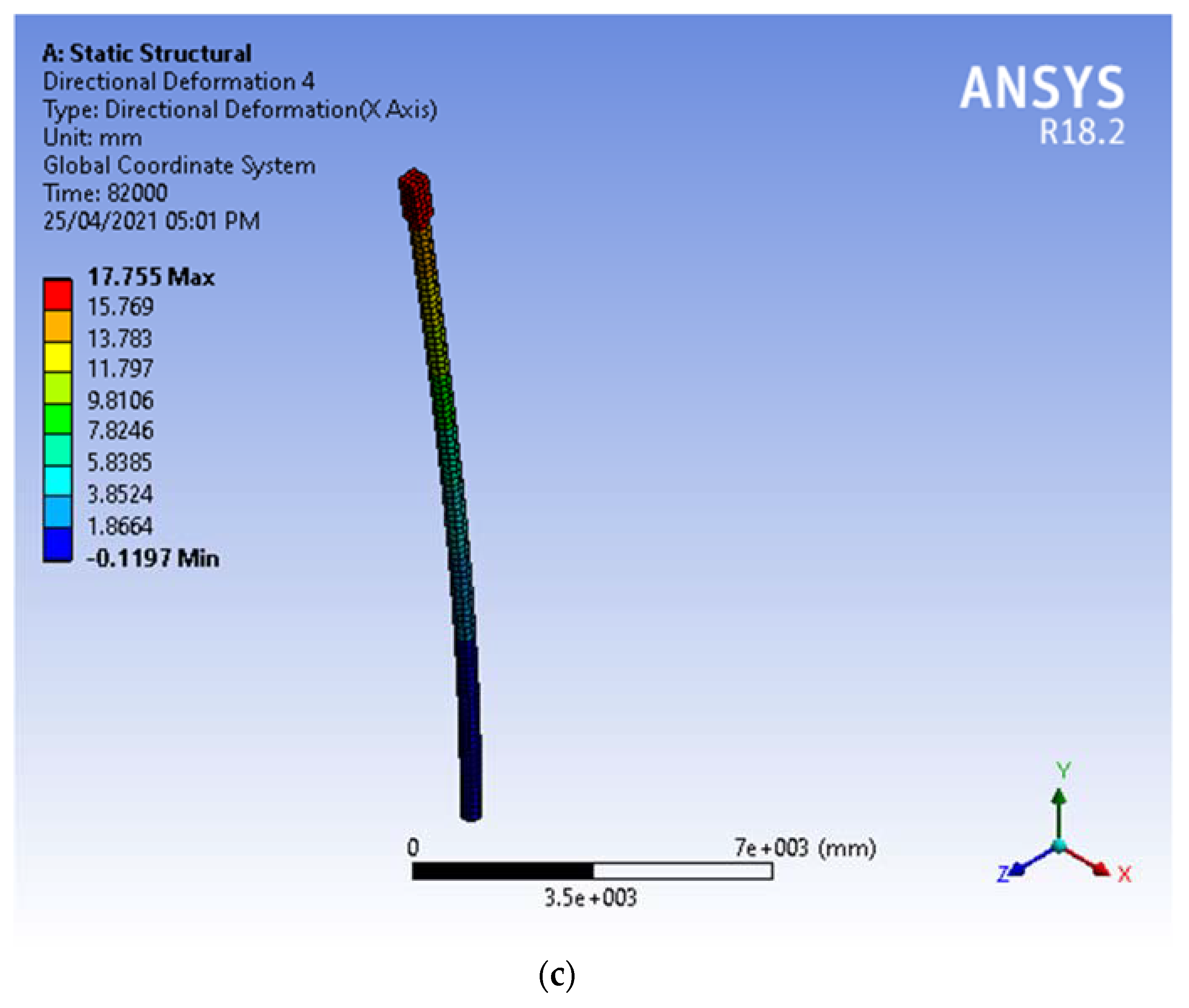
Figure 3 presents the computed pile head deflections versus applied lateral forces for both the analytical solution and FE solution with ANSYS software. The figure indicates that the results of the proposed analytical solution are closer to the results from the FE method. The lateral deflection obtained by the ANSYS workbench 18.2 for different lateral loads, 2, 75.5, and 82 kN are shown in
Figure 4. The captured results obtained from
Figure 3 are compared with those obtained by proposed analytical method as shown in
Table 3. The presented results clearly indicate excellent agreement with the FE solution.
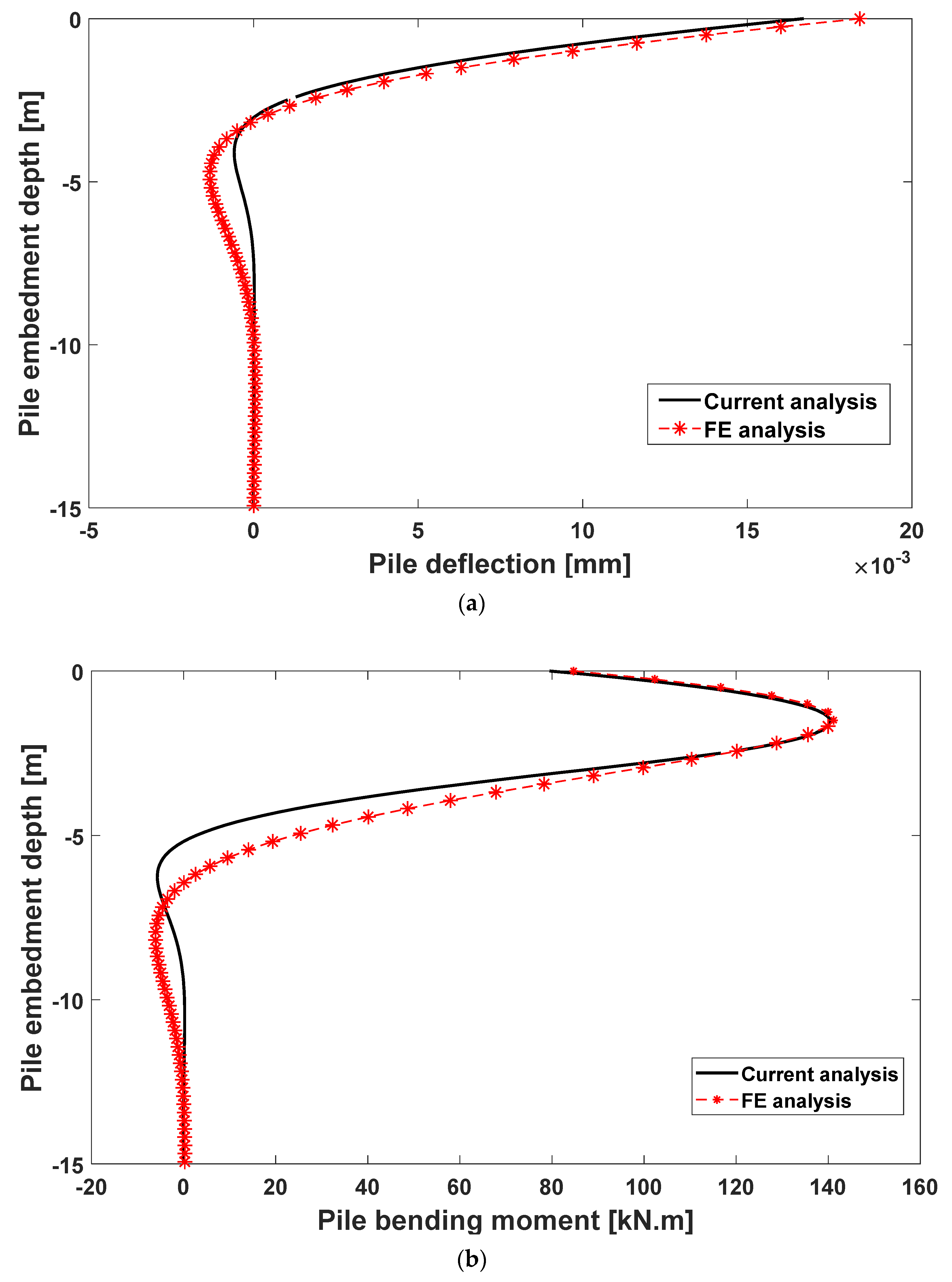
Additionally, to ensure that the proposed solution produces a reliable pile deflection and bending moment not only at the pile head but also for the entire pile length, the lateral deflection and bending moment distribution along the pile shaft are presented and compared with the results of the FE analysis as shown in
Figure 5.
The captured peak lateral deflection and bending moment obtained from the analytical solution are 16.710 mm and 140.459 kN·m, respectively, while the corresponding values obtained from the FE analysis are 17.809 mm and 141.053 kN·m, respectively. The results clearly indicate the agreement between the analytical and FE solutions in calculating peak value for design purposes.
Additionally, it is observed that the lateral deflection and bending moment profiles obtained using the proposed analytical method reach a good agreement with the FE solution.
5. Conclusions
An analytical solution of the lateral response of an infinite pile embedded in homogeneous elasto-plastic soil deposits has been proposed in the current study. The solution is based on conceptual assumptions of the Winkler model which treat the pile as a flexible beam and soil restraint surrounding the pile as a series of non-linear independent springs. The flexural differential equation describing the response of the soil–pile system was solved analytically. Additionally, the location at which the maximum bending moment occurs, and the magnitude of that maximum bending moment along the pile were obtained from the analysis. For verification of the proposed analytical procedure, the obtained results are compared with the FE results, carried out using ANSYS software, showing excellent agreements. The proposed exact solution could efficiently provide a better approach for structural designers to predict the non-linear responses of laterally loaded free-head long piles embedded in clay soil deposits with a uniform subgrade reaction modulus. Additionally, the proposed analytical solution has the advantage that it can provide a better approach for engineers to analyse and design the piles subjected to lateral loads without resorting to a 3D FE analysis, which is time consuming. Consequently, the mathematical forms of the theoretical solutions can be easily applied in practice as an alternative approach to analyse and design laterally loaded long piles.
It is emphasized that the simplified analytical solution obtained in this study is limited by the linearity of the soil–pile system, which often significantly affects the overall responses of the pile and the soil. Therefore, the proposed solution must be modified before applied to a non-linear case. Moreover, further investigation and analyses are needed to analyse the laterally loaded long piles in soil with variable subgrade reactions with depth, or for piles embedded in multilayered soil.


