An Asymptotic Solution for Call Options on Zero-Coupon Bonds

Abstract

We present an asymptotic solution for call options on zero-coupon bonds, assuming a stochastic process for the price of the bond, rather than for interest rates in general. The stochastic process for the bond price incorporates dampening of the price return volatility based on the maturity of the bond. We derive the PDE in a similar way to Black and Scholes. Using a perturbation approach, we derive an asymptotic solution for the value of a call option. The result is interesting, as the leading order terms are equivalent to the Black–Scholes model and the additional next order terms provide an adjustment to Black–Scholes that results from the stochastic process for the price of the bond. In addition, based on the asymptotic solution, we derive delta, gamma, vega and theta solutions. We present some comparison values for the solution and the Greeks.

1. Introduction

Black and Scholes’ [1] solution for European style options assumes a geometric Brownian motion process for the underlying stock price. Many additional asset classes were also assumed to follow this process, and so the Black-Scholes model was used to price options on a variety of asset classes. Since many asset classes have no maturity (stocks, commodity prices, foreign exchange rates), this process seems reasonable. However, it was clear from the outset that this process would not work for most bond prices. To price bonds, and other interest rate securities, researchers turned to modeling interest rates and using the resulting rates to price interest rate securities and their related derivative securities.

In this paper, we propose a process for a zero-coupon bond price directly, and using that process, we derive a partial differential equation (PDE) and an asymptotic solution for a call option on the bond. Our approach of modeling bond price dynamics rather than interest rate dynamics offers several important advantages. First, we are not restricted to assumptions regarding the relationship of interest rates in a term structure, that is, we do not need to assume rates fit a model, such as “Preferred Habitat.” Second, modeling the bond dynamics is computationally simpler than many spot and term structure models with multiple factors. In order for spot and term structure models to provide for reasonable representation of interest rate dynamics, the models often require multiple uncertainty terms with non-constant volatility. This results in computationally complex formulations, which normally require numerical solutions. Finally, the resulting solution to our formulation is similar to the familiar Black–Scholes model for European style call options on stocks. While there are advantages and disadvantages to every approach, modeling bond dynamics directly is more closely aligned with the nature of trading in the asset itself; bonds, like stocks, trade in denominated currencies (models that focus on interest rate dynamics are one-step removed, in the sense that they are inputs into a pricing process for an underlying asset. If we were examining stocks, for instance, one possible way to price options on stocks would be to model dynamics for factors that affect stock price—perhaps a stochastic process for the market risk premium, as an example—then derive a stock price and then price the option. Black and Scholes decided to model the stock price directly. In that vein, we are returning to directly modeling the bond’s price). In this fashion, our approach adds to the literature on option pricing where the underlying asset price is modeled directly.

In what follows, we provide a short review of extant interest rate models. We discuss a stochastic process for the bond price and derive the PDE. We then present the asymptotic solution for a European style call option. Finally, we discuss the properties of our model, including the commonly used Greeks.

2. Previous Literature: Interest Rate Models

Vasicek [2], Rendleman and Bartter [3], Black, Derman and Toy [4], Black and Karasinski [5], are examples of short rate models, where parameters are generally chosen to make the evolution of the spot rate fit the current term structure. In Vasicek [2], the bond’s price follows from an evolution of a spot rate that follows a Markov process. Vasicek [2] uses the specific example of an Ornstein–Uhlenbeck process to derive the representation of the bond price. Rendleman and Bartter [3] discuss the pricing of bond options where interest rates follow a binomial process with parameters chosen so that the price relative (ratio of) interest rates approximate a lognormal distribution. In the study of Black, Derman, and Toy [4], all security prices and rates depend on only one factor, the short rate. The current structure of long rates and their estimated volatilities are used to construct a tree of possible future short rates, which may then be used to value interest-rate-sensitive securities. Black and Karasinski [5] present a short-term interest rate one-factor model for bond and option pricing that allows the target rate, mean reversion and local volatility to vary deterministically through time. The distribution of possible short rates is lognormal in their model, so the rate will not fall below zero. Jamshidian [6] derives a closed-form solution for an option on a zero-coupon bond assuming the process developed by Vasicek [2].

The studies of Ho and Lee [7], Heath, Jarrow and Morton [8,9], Duffie and Kan [10], Brace, Gatarek, and Muiela [11], and Musiela and Rutkowski [12] are examples of term structure models. These models take a given term structure and model its behavior. Ho and Lee [7] derive an arbitrage free discrete trading economy, where bond prices fluctuate according to a single factor path independent binomial process. Securities are priced relative to a term structure of interest rates (spot rate and forward rates). The path independence condition is equivalent to constant volatility in the forward rate process. Heath, Jarrow, and Morton [8,9] develop a framework for pricing interest rate claims based on the term structure of forward rates. The model (HJM for convenience) treats the entire forward rate curve at a point in time as an input, and evolves the curve according to a stochastic process. The stochastic process for the forward rate is the sum of a simple diffusion and a deterministic drift, and is more general than Ho and Lee [7]; the forward rate process may have non-constant volatilities for instance. Duffie and Kan [10] analyze a multifactor model of the term structure, where the yield factors form a Markov process. In Brace, Gatarek, and Muiela [11], a class of term structure models with a volatility of the lognormal type is analyzed in the general HJM framework. The corresponding market forward rates do not explode and are positive and mean reverting. Musiela and Rutkowski [12] describe the properties and problems associated with continuous-time presentations of term-structure models and specify the general properties for wide classes of models.

Two highly recommended, and excellent discussions of interest rate models, and their associated problems, are provided by Björk and Gaspar [13] and Rebonato [14]. Björk and Gaspar present a collection of important topics and conditions for arbitrage free pricing of interest rate claims, including a discussion of the market price of risk, short-rate models, and term structure models. For those just starting to study interest rate models, Section 1 and Section 2 provide a host of useful theorems and definitions. In addition, there is an excellent discussion on the difficulties of operationalizing these models, and how to approach the realization of essentially infinite-dimensional models in finite dimensional space. Rebonato discusses the evolution of interest-rate models from the early short-rate models to more recent developments in term-structure models and provides a far more comprehensive discussion than what can be provided here. In fact, two quotes from Rebonato provide the inspiration for this work:

Therefore, while today’s models are indubitably more effective (at least in certain respects) than the early ones, and, therefore, one can certainly speak of an ‘evolution’ of interest-rate models, this does not necessary imply that certain choices, abandoned in the past, might not have ultimately led a more fruitful description of interest-rate derivatives products if they had been pursued more actively.

[14] (p. 672)

As well as the following:

As for the log-normal assumption for the bond price, this was partly satisfactory, because it did not constrain the price to be smaller than face value, thereby assigning a non-zero probability to negative interest rates…What gave greater discomfort, however, was the so-called pull-to-par problem.

[14] (p. 683)

The pull-to-par issue is an important facet of bond returns, as noted in such works as that of Esquível, Gaspar, and Beleza Sousa [15]. Esquível et al. use pull-to-par returns to analyze implicit default propensities from observed bond prices. While their paper does not explicitly put forth a stochastic process to create bond prices, and instead is based on market data, they do note that one could imagine a stochastic process that might create price realizations:

Although this is not necessary for what follows, we may suppose that it is a stochastic process–defined on a complete probability space $\left(\Omega ,A,\mathbb{P}\right)$–from which some realization is observed.

[15] (p. 82)

The valuation of simple contingent claims under simple continuous time models is no longer novel; however, we believe that there is value in the return to the “pull-to-par” issue and the pursuit of a path “abandoned in the past.” We propose an approach based on the bond’s price, rather than a set of interest rates/forward rates, that better captures the pull-to-par dynamics of a bond than the traditional geometric Brownian motion (we do note that the pull-to-par problem can be handled in the classical short-rate and term-structure models of interest rates, and so when we are referring to addressing the pull-to-par problem, it is with respect to a model of bond price dynamics. We thank an anonymous referee for pointing out our need to clarify this point).

By going back to the bond’s price, we are not limited to processes for interest rates that, due to computational complexities, are typically limited to three factors (or less) to characterize a yield curve (partly to avoid overfitting problems and to allow for some tractability). There is no need to fit a curve or restrict the evolution of rates so that the resulting term structure fits with observable bond prices. By starting with a process for the bond, we can, in a fashion similar to Black and Scholes develop a solution that does not require assumptions about the term structure or the relation of rates across maturities. Our model would also be an example of a stochastic process that could characterize zero coupon bond prices as described by Esquível, Gaspar, and Beleza Sousa [15].

3. Derivation of Bond Options on Zero-Coupon Bonds

3.1. A Process for Zero-Coupon Bonds

To begin, we assume that the zero-coupon bond’s price before maturity can be any positive value, including values higher than par (nominally negative interest rates). We make very few assumptions on the implied interest rates other than rates are made up of two components: a risk-free rate (time value of money) and a risk premium (if the bond is risky). We assume that interest rates in a term structure may or may not be related to such frameworks as those of the “expectations hypothesis,” “preferred habitat theory,” “liquidity preference,” or “market segmentation,” though we are not specifying any specific structure (an excellent discussion of these can be found in the study of Cox, Ingersoll, and Ross [16] in the introduction). As such, the rate implied by our zero-coupon bond price (the process of which is given later) can be expressed as an average of a current short rate and future short rates, if so chosen, that is, the bond’s current price reflects the term structure to its maturity at the current time.

3.2. Model Definition

We start with dynamics for the zero-coupon bond price.

$$dB=B\left(\frac{ln\left(\frac{F}{B}\right)}{T_B-t}\right)dt+\sigma B\left(\frac{T_B-t}{T_B}\right)dz$$

(1)

where B is the price of a zero-coupon bond that is worth F at maturity. T_B is the maturity time for the bond, t is the current time, z is a Brownian motion, and σ is the volatility of the bond’s return at full duration (initial duration, which for the zero-coupon bond equals the bonds maturity). The dz and σ are unique for each bond maturity, and are not to be seen as common terms across all maturities (as noted by an anonymous referee, there is empirical research indicating that only three or four independent stochastic components are needed to describe the market. Our assumption of different Brownian motions across the maturities is made to ensure no arbitrage). The first term (drift term) represents the pull-to-par effect that takes place if the implied interest rate on the bond does not change as time changes. The second term (shock term) represents the riskiness of the bond, which is a function of its duration (in this case, the remaining percent of initial duration). Therefore, the volatility constant, σ, is scaled down over time as the bond’s remaining time to maturity becomes shorter. For simplicity of discussion, we refer to the model as the pull-to-par model (or PTP). Of course, there are many different ways in which the dynamics could be proposed. We chose to try and capture two important characteristics in the bond price dynamics (pull-to-par and duration), while adopting a form that would adjust for the problems of the Black and Scholes geometric Brownian motion described in Rebonato. Yet, the dynamics we chose are still suggestive of that in Black and Scholes, so the derivation and solution will be familiar to many.

While our focus is on characterizing risky bonds, we do note that our process could conceptually represent a risk-free bond (a somewhat trivial result but important in the resulting model, which, like Black and Scholes, has a constant risk-free rate as part of the solution). In the case of a conceptually true risk-free bond, $B_{rf}$, the volatility for it would be ${\sigma }_{rf}=0$, (there would be no uncertainty of any type—no risk premiums) and the term in (1) would result in the bond earning a constant continuously compounded risk-free rate, $r$ (note, the ODE $dB=B\frac{ln\left(\frac{F}{B}\right)}{\left(T_B-t\right)}dt$ has the general solution $B=F{e}^{K\left(t-T_B\right)}$ where K is an arbitrary constant).

In our model, in order for there to be no arbitrage, we need only assume that a risky bond, $B\left(0,T\right)$, with volatility σ, has the following properties:

$$B\left(0,T\right)<B_{rf}\left(0,T\right), \mathrm{and} \sigma >0$$

The resulting initial (expected) rate of return on the risky bond, $r_B$, could therefore be expressed as follows:

$$r_B=r+\lambda$$

where $\lambda$ is the risk-premium(s) for bond B. The process in (1) therefore can represent both risk-free and risky bonds. Since our formulation is general, one could imagine the risk-premium representing such concepts as inflation risk, liquidity risk, default risk, etc. (or some combination of these and others). There are some limits to our model in conceptualizing the default risk since we do not specifically cover the recovery rates for bonds in default but, as noted later, our model would work in situations where the recovery rate is below the strike on the option.

The following exposition on the derivation of the governing PDE is for those interested in seeing the steps in comparison to the well-known Black–Scholes solution to a European option on stocks. Those familiar with the derivation might prefer to move directly to the solution in Section 4.

Suppose that there is a European style call option on this bond (a function of the bond price and time), denoted as follows:

$$C=C\left(B,t\right)$$

(2)

By Ito’s Lemma, with Equation (1), we have the following:

$$dC=\left\{C_t+C_{B}B\left(\frac{ln\left(\frac{F}{B}\right)}{T_B-t}\right)+\frac{1}{2}{C}_{BB}{\sigma }^2{B}^2{\left(\frac{T_B-t}{T_B}\right)}^2\right\}dt+C_B\sigma B\left(\frac{T_B-t}{T_B}\right)dz$$

(3)

where C_t and C_B are partial derivatives of C with respect to t and B, respectively, and C_BB is the second partial derivative of C with respect to B.

We can form a hedge portfolio by combining N_B shares of the bond and N_C call options. The value of the hedge portfolio (V_H) is given by the following:

$$V_H=N_{B}B+N_{C}C$$

(4)

Differentiating (4) and substituting for dB from (1) and dC from (3) and rearranging, we obtain the following:

$$d{V}_H=N_C{C}_{t}dt+\left\{N_B+N_C{C}_B\right\}B\left(\frac{ln\left(\frac{F}{B}\right)}{T_B-t}\right)dt+\frac{1}{2}{N}_C{C}_{BB}{\sigma }^2{B}^2{\left(\frac{T_B-t}{T_B}\right)}^{2}dt+\left\{N_B+N_C{C}_B\right\} \sigma B\left(\frac{T_B-t}{T_B}\right)dz$$

(5)

A perfectly hedged portfolio should be risk-free and earn the risk-free rate, r; therefore, the following holds:

$$d{V}_H=r{V}_{H}dt$$

(6)

To hedge, we need to set the following condition:

$$N_B+N_C{C}_B=0$$

(7)

Substituting (4), (6) and (7) into (5), and dividing through by dt and N_C, we obtain the following:

$$rC-rB{C}_B-\frac{1}{2}{\sigma }^2{B}^2{\left(\frac{T_B-t}{T_B}\right)}^2{C}_{BB}-C_t=0,$$

(8)

for $0\le B<\infty$, and $0\le t\le T_C$.

In addition, we have the following initial and boundary conditions for (8):

$$C\left(B,T_C\right)=Max\left(B-E,0\right)$$

(8a)

$$C\left(0,t\right)=0$$

(8b)

where E is the exercise price of the call option (Condition 8b could also be written as C(γ,t) = 0 for recovery value γ, where 0 ≤ γ < E < 1. Note, our model would not be appropriate in the case of default where the recovery value γ has the following property 0 ≤ E < γ < 1).

4. Solution

Under the assumption that $T_B$ is much larger than $T_C$ (i.e., $\frac{T_C}{T_B}\ll 1$), we use a regular perturbation method to find an asymptotic solution for (8). For the mathematical definition of $\frac{T_C}{T_B}\ll 1$ and the asymptotic solution procedure, see Kevorkian and Cole [17]. We further assume that $T_C=O\left(1\right)$ and look for an asymptotic solution of the following form:

$$C\left(B,t;T_B\right)=C_0\left(B,t\right)+\frac{1}{T_B}{C}_1\left(B,t\right)+O\left(\frac{1}{T_B{}^2}\right)$$

(9)

Which, for our PDE and its initial and boundary conditions, is equal to the following:

$$BN\left(d_1\right)-e^{-r\left(T_C-t\right)}EN\left(d_2\right)+\frac{1}{T_B}E{e}^{\left(\left(\frac{1-\alpha }{2}\right)ln\left(\frac{B}{E}\right)-\frac{{\left(1+\alpha \right)}^2}{4}\left(T_C-t\right)\frac{{\sigma }^2}{2}\right)}\left(M\right)+O\left(\frac{1}{T_B{}^2}\right)$$

The derivation of this solution is rather involved. We detail it in the Appendix A and omit it here for brevity. If we let $\tau =T_C-t$ (time moves forward), this becomes the following:

$$BN\left(d_1\right)-e^{-r\left(\tau \right)}EN\left(d_2\right)+\frac{1}{T_B}E{e}^{\left(\left(\frac{1-\alpha }{2}\right)ln\left(\frac{B}{E}\right)-\frac{{\left(1+\alpha \right)}^2{\sigma }^2\tau }{8}\right)}\left(M\right)+O\left(\frac{1}{T_B{}^2}\right)$$

(10)

where M is defined as follows:

$$M=\left\{\left(\frac{\tau }{2}-T_C\right)\sqrt{\frac{{\sigma }^2\tau }{2\pi }}{e}^{-\frac{{\left(ln\left(\frac{B}{E}\right)\right)}^2}{2{\sigma }^2\tau }}+\frac{{\left(ln\left(\frac{B}{E}\right)\right)}^2}{8{\sigma }^2}\left(\left|ln\left(\frac{B}{E}\right)\right|-1\right)erfc\left(\frac{\left|ln\left(\frac{B}{E}\right)\right|}{2\sqrt{\frac{{\sigma }^2}{2}\tau }}\right)\right\}$$

Additionally, N(z) is defined as follows:

$$N\left(z\right)=\frac{1}{\sqrt{2\pi }}{{\displaystyle \int }}_{-\infty }^z{e}^{-\frac{w^2}{2}}dw$$

and d₁ and d₂ are defined as follows:

$$d_1=\frac{\left\{ln\left(\frac{B}{E}\right)+\left(r+\frac{1}{2}{\sigma }^2\right)\tau \right\}}{\sigma \sqrt{\tau }}$$

$${\mathit{d}}_{\mathbf{2}}={\mathit{d}}_{\mathbf{1}}- \mathit{\sigma }\sqrt{\mathit{\tau }}=\frac{\left\{\mathit{l}\mathit{n}\left(\frac{\mathit{B}}{\mathit{E}}\right)+\left(\mathit{r}-\frac{\mathbf{1}}{\mathbf{2}}{\mathit{\sigma }}^{\mathbf{2}}\right)\mathit{\tau }\right\}}{\mathit{\sigma }\sqrt{\mathit{\tau }}}$$

We also have α defined as:

$$\alpha =\frac{2r}{{\sigma }^2}$$

and erfc(z) as:

$$erfc\left(z\right)=\frac{2}{\sqrt{\pi }}{{\displaystyle \int }}_z^{\infty }{e}^{-y^2}dy$$

Discussion of Results

The first two terms in the solution, (Equation (10)) is equivalent to the Black–Scholes model. The additional terms provide an adjustment to Black–Scholes that results from the pull-to-par effect and dampening effect on volatility that are present in the original stochastic Equation (1). In particular, the third term represents the leading order approximation to that adjustment under the assumption that $T_B$ is much larger than $T_C$. Mathematically, the solution in (10) decomposes the PTP model into a descending order of components with the leading order $O\left(1\right)$, a Black–Scholes model. This is given by the first two terms in (10) and it is governed by the homogeneous Black–Scholes Equation (A1a), subject to the initial and boundary conditions (8a, b). The next order $O\left(\frac{1}{T_B}\right)$ in (10), which is the leading adjustment to the Black–Scholes model, is governed by a forced Black–Scholes Equation (A1b), subject to zero initial and boundary conditions. The forcing term here is given by the gamma of the Black–Scholes model, multiplied by ${\sigma }^2{B}^{2}t$. Given these effects, the PTP model results in a solution that is less than that of a pure Black–Scholes geometric Brownian motion solution.

To illustrate the differences, we have included a few computations, which are not meant to be exhaustive (see Table 1). Using the daily 20-year constant maturity treasury yields for the year 2020 (Treasury.Gov, 1 April 2021), we created daily zero-coupon bond prices, from which we then derived the estimated daily price returns. The choice of treasury data was two-fold: (1) the data are easily accessed by all interested, and (2) since our paper is not focused on any particular set of risk premiums, treasury bonds, while generally considered default free, are nonetheless risky (it is generally commonly held that treasury debt has at least inflation risk). The data were largely used to give us a set of inputs for illustrative purposes. The annualized standard deviation of the returns serves as a basis for the volatility input in the tables that follow. The annualized standard deviation of the hypothetical 20-year zero-coupon bond (assuming 256 trading days) was 20.20%. Given this, table computations have volatilities of 15%, 20%, and 25% for the option values and the Greeks. For the year 2020, short-term treasury rates (3 months, 6 months, and 1 year) ranged from near zero to just over 1.5%, with an average of slightly below 0.5%. Based on this, an input of 0.5% for the short-term risk-free rate was used as an input to the model.

Table 1. Comparison of PTP values to Black–Scholes: strike price 80, risk-free rate 0.5%, bond maturity 20 years.

Volatility 15%
	Option Maturity 0.25 Years		Option Maturity 0.5 Years		Option Maturity 1 Year
Bond Price	PTP	Black–Scholes	PTP	Black–Scholes	PTP	Black–Scholes
72	0.1635	0.2140	0.6151	0.7087	1.6037	1.7065
76	0.8201	0.8820	1.6655	1.7368	3.0303	3.0701
80	2.3971	2.4419	3.4379	3.4801	4.9730	4.9730
84	4.9643	5.0273	5.8893	5.9606	7.3626	7.4004
88	8.3351	8.3938	8.9581	9.0560	10.1888	10.2867
Volatility 20%
72	0.5158	0.5835	1.3647	1.4599	2.9080	2.9788
76	1.4694	1.5393	2.6761	2.7496	4.5372	4.5614
80	3.1787	3.2384	4.5485	4.6047	6.5580	6.5580
84	5.6463	5.7183	6.9416	7.0165	8.9257	8.9488
88	8.7695	8.8449	9.8153	9.9148	11.6266	11.6935
Volatility 25%
72	0.9935	1.0738	2.2248	2.3227	4.2850	4.3357
76	2.1610	2.2414	3.7128	3.7936	6.0542	6.0704
80	3.9599	4.0345	5.6578	5.7280	8.1394	8.1394
84	6.3730	6.4564	8.0254	8.1087	10.5079	10.5233
88	9.3322	9.4207	10.7848	10.8881	13.1461	13.1937

In addition to the hypothetical values, an analysis of the contribution of the terms $O\left(1\right)$ and $O\left(\frac{1}{T_B}\right)$ are provided in Table 2. As noted earlier, our approximation solution assumes that the maturity of the bond is considerably larger than that of the option.

Table 2. Contribution of terms to PTP values: strike price 80, risk free rate 0.5%.

Bond Maturity
Bond Price	Volatility	Option Maturity	5 Years	5 Years	10 Years	10 Years	20 Years	20 Years	30 Years	30 Years
			O(1)	O(1/T_B)	O(1)	O(1/T_B)	O(1)	O(1/T_B)	O(1)	O(1/T_B)
72	15%	0.25	57.42%	42.58%	72.95%	27.05%	84.36%	15.64%	89.00%	11.00%
72	20%	0.50	79.32%	20.68%	88.47%	11.53%	93.88%	6.12%	95.84%	4.16%
72	25%	1.0	82.91%	17.09%	90.66%	9.34%	95.10%	4.90%	96.68%	3.32%
80	15%	0.25	97.61%	2.39%	98.79%	1.21%	99.39%	0.61%	99.59%	0.41%
80	20%	0.50	95.35%	4.65%	97.62%	2.38%	98.79%	1.21%	99.19%	0.81%
80	25%	1.00	91.16%	8.84%	95.37%	4.63%	97.63%	2.37%	98.41%	1.59%
88	15%	0.25	97.90%	2.10%	98.94%	1.06%	99.47%	0.53%	99.64%	0.36%
88	20%	0.50	96.14%	3.86%	98.03%	1.97%	99.01%	0.99%	99.34%	0.66%
88	25%	1.00	93.25%	6.75%	96.51%	3.49%	98.22%	1.78%	98.81%	1.19%

We illustrate the contribution for a range of bond maturities against option maturities of 3 months, 6 months and 1 year. As the bond maturity increases, the contribution of the $O\left(\frac{1}{T_B}\right)$ generally decreases.

5. Properties of Greeks

Based on the solution in Equation (10), we derived the standard “Greeks” associated with the call option. The solutions are presented below:

The call option’s delta is equal to the following:

$$\begin{array}{cc}\frac{\partial C}{\partial B}= N\left(d_1\right)& +\frac{1}{\sigma \sqrt{2\pi \tau }}\left(e^{\left(-\frac{d_1{}^2}{2}\right)}-e^{-r\tau }\frac{E}{B}{e}^{\left(-\frac{d_2{}^2}{2}\right)}\right)\\ & +\frac{E}{T_{B}B}{e}^{\left(\left(\frac{1}{2}-\frac{r}{{\sigma }^2}\right)ln\left(\frac{B}{E}\right)-\frac{{\left(\sigma +\frac{2r}{\sigma }\right)}^2}{8}\tau \right)}\left\{Q_1\frac{e^{\left(\raisebox{1ex}{$-{\left(ln\left(\frac{B}{E}\right)\right)}^2$}\!\left/ \!\raisebox{-1ex}{$2{\sigma }^2\tau $}\right.\right)}}{4\sqrt{2\pi }}+Q_2\frac{erfc\left(\frac{\left|ln\left(\frac{B}{E}\right)\right|}{\sigma \sqrt{2\tau }}\right)}{8{\sigma }^2}\right\}+O\left(\frac{1}{T_B^2}\right)\end{array}$$

where

$$Q_1=\left[\left(\frac{2r}{\sigma }-\sigma \right)\left(2T_C-\tau \right)\sqrt{\tau }+\frac{2ln\left(\frac{B}{E}\right)\left(2T_C-\tau \right)}{\sigma \sqrt{\tau }}-\frac{ln\left(\frac{B}{E}\right)\left({\left(ln\left(\frac{B}{E}\right)\right)}^2-\left|ln\left(\frac{B}{E}\right)\right|\right)}{{\sigma }^3\sqrt{\tau }}\right]$$

and

$$Q_2=\left[\left(\frac{1}{2}-\frac{r}{{\sigma }^2}\right){\left(ln\left(\frac{B}{E}\right)\right)}^2\left(\left|ln\left(\frac{B}{E}\right)\right|-1\right)+ln\left(\frac{B}{E}\right)\left(3\left|ln\left(\frac{B}{E}\right)\right|-2\right)\right]$$

As with the options value, we also calculated values for the call’s delta. Table 3 illustrates these for the same strike, short rate, and set of volatilities and option maturities.

Table 3. Comparison of PTP deltas to Black–Scholes: strike price 80, risk-free rate 0.5%, bond maturity 20 years.

Volatility 15%
	Option Maturity 0.25 Years		Option Maturity 0.5 Years		Option Maturity 1 Year
Bond Price	PTP	Black–Scholes	PTP	Black–Scholes	PTP	Black–Scholes
72	0.0807	0.0884	0.1794	0.1796	0.2890	0.2762
76	0.2674	0.2644	0.3518	0.3420	0.4238	0.4076
80	0.5214	0.5216	0.5304	0.5305	0.5431	0.5431
84	0.7558	0.7595	0.6945	0.7042	0.6527	0.6677
88	0.9127	0.9074	0.8328	0.8353	0.7583	0.7715
Volatility 20%
72	0.1567	0.1608	0.2586	0.2557	0.3554	0.3439
76	0.3288	0.3262	0.3986	0.3919	0.4581	0.4477
80	0.5246	0.5249	0.5350	0.5352	0.5497	0.5497
84	0.7057	0.7090	0.6607	0.6676	0.6342	0.6439
88	0.8470	0.8451	0.7726	0.7771	0.7151	0.7263
Volatility 25%
72	0.2182	0.2205	0.3140	0.3108	0.4003	0.3911
76	0.3695	0.3677	0.4301	0.4256	0.4832	0.4760
80	0.5285	0.5289	0.5405	0.5408	0.5576	0.5576
84	0.6757	0.6783	0.6425	0.6475	0.6264	0.6331
88	0.7986	0.7981	0.7351	0.7395	0.6919	0.7006

As with the value, the delta is generally a bit lower than that of an equivalent Black–Scholes model. Graphically, Figure 1 and Figure 2 present the deltas for differing option maturities and volatilities, respectively.

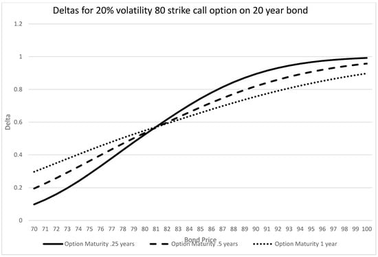
Figure 1. PTP deltas at different option maturities.

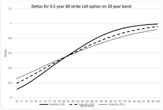
Figure 2. PTP deltas at different volatilities.

The call option’s gamma is equal to the following:

$$\begin{array}{cc}\frac{{\partial }^{2}C}{\partial B^2}=\frac{e^{\left(-\frac{d_1{}^2}{2}\right)}}{B\sigma \sqrt{2\pi \tau }}& \left(1-\frac{d_1}{\sigma \sqrt{\tau }}\right)+e^{\left(-r\tau -\frac{d_2{}^2}{2}\right)}\frac{E}{B^2}\raisebox{1ex}{$\left(1+\frac{d_2}{\sigma \sqrt{\tau }}\right)$}\!\left/ \!\raisebox{-1ex}{$\left(\sigma \sqrt{2\pi \tau }\right)$}\right.\\ & +\frac{E}{T_B{B}^2}{e}^{\left(\left(\frac{1}{2}-\frac{r}{{\sigma }^2}\right)ln\left(\frac{B}{E}\right)-\frac{{\left(\sigma +\frac{2r}{\sigma }\right)}^2}{8}\tau \right)}[\left(-\frac{1}{2}-\frac{r}{{\sigma }^2}\right)\left(Q_1\frac{e^{\left(\raisebox{1ex}{$-{\left(ln\left(\frac{B}{E}\right)\right)}^2$}\!\left/ \!\raisebox{-1ex}{$2{\sigma }^2\tau $}\right.\right)}}{4\sqrt{2\pi }}+Q_2\frac{erfc\left(\frac{\left|ln\left(\frac{B}{E}\right)\right|}{\sigma \sqrt{2\tau }}\right)}{8{\sigma }^2}\right)\\ & +\frac{e^{\left(\raisebox{1ex}{$-{\left(ln\left(\frac{B}{E}\right)\right)}^2$}\!\left/ \!\raisebox{-1ex}{$2{\sigma }^2\tau $}\right.\right)}}{4\sqrt{2\pi }}\left(B\frac{\partial Q_1}{\partial B}-\frac{Q_{1}ln\left(\frac{B}{E}\right)}{{\sigma }^2\tau }-\frac{Q_3}{{\sigma }^3\sqrt{\tau }}\right)+B\frac{\partial Q_2}{\partial B}\frac{erfc\left(\frac{\left|ln\left(\frac{B}{E}\right)\right|}{\sigma \sqrt{2\tau }}\right)}{8{\sigma }^2}]+O\left(\frac{1}{T_B^2}\right)\end{array}$$

where

$$Q_3=\left(\frac{1}{2}-\frac{r}{{\sigma }^2}\right)ln\left(\frac{B}{E}\right)\left\{{\left(ln\left(\frac{B}{E}\right)\right)}^2-\left|ln\left(\frac{B}{E}\right)\right|\right\}+3{\left(ln\left(\frac{B}{E}\right)\right)}^2-2\left|ln\left(\frac{B}{E}\right)\right|$$

and

$$\frac{\partial Q_1}{\partial B}=\frac{1}{B}\left(\frac{4T_C-2\tau }{\sigma \sqrt{\tau }}-\frac{3{\left(ln\left(\frac{B}{E}\right)\right)}^2-2\left|ln\left(\frac{B}{E}\right)\right|}{{\sigma }^3\sqrt{\tau }}\right)$$

and

$$\frac{\partial Q_2}{\partial B}=\frac{1}{B}\left\{\left(\frac{1}{2}-\frac{r}{{\sigma }^2}\right)ln\left(\frac{B}{E}\right)\left(3\left|ln\left(\frac{B}{E}\right)\right|-2\right)+6\left|ln\left(\frac{B}{E}\right)\right|-2\right\}$$

Table 4 presents the gamma values with the same underlying data used for the values and deltas.

Table 4. Comparison of PTP gammas to Black–Scholes: strike price 80, risk-free rate 0.5%, bond maturity 20 years.

Volatility 15%
	Option Maturity 0.25 Years		Option Maturity 0.5 Years		Option Maturity 1 Year
Bond Price	PTP	Black–Scholes	PTP	Black–Scholes	PTP	Black–Scholes
72	0.0311	0.0297	0.0375	0.0343	0.0335	0.0310
76	0.0601	0.0574	0.0464	0.0456	0.0328	0.0341
80	0.0607	0.0664	0.0405	0.0469	0.0261	0.0331
84	0.0516	0.0494	0.0394	0.0388	0.0277	0.0288
88	0.0266	0.0251	0.0289	0.0266	0.0245	0.0229
Volatility 20%
72	0.0356	0.0339	0.0333	0.0316	0.0263	0.0256
76	0.0485	0.0474	0.0356	0.0357	0.0247	0.0260
80	0.0468	0.0498	0.0317	0.0351	0.0209	0.0247
84	0.0417	0.0408	0.0304	0.0306	0.0210	0.0222
88	0.0284	0.0271	0.0251	0.0240	0.0193	0.0189
Volatility 25%
72	0.0342	0.0329	0.0286	0.0278	0.0214	0.0213
76	0.0402	0.0397	0.0288	0.0292	0.0198	0.0210
80	0.0380	0.0398	0.0259	0.0281	0.0173	0.0197
84	0.0345	0.0341	0.0247	0.0250	0.0169	0.0179
88	0.0265	0.0256	0.0214	0.0209	0.0157	0.0158

As with the delta, the gamma is also somewhat lower than that of an equivalent Black–Scholes model. Graphically, Figure 3 and Figure 4 present the gammas for differing option maturities and volatilities, respectively.

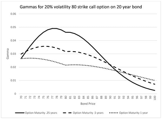
Figure 3. PTP gammas at different option maturities.

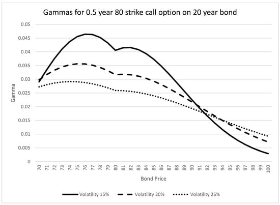
Figure 4. PTP gammas at different volatilities.

The gamma results present a “corner” for the at-the-money options. This is likely due to the method of derivation, i.e., the approximate solution. In solving the differential equation at order $O\left(\frac{1}{T_B}\right)$, the Laplace transform method was used, and the solutions for intervals x > 0 and x < 0 were obtained first, then matched at x = 0 (i.e., B = 80).

In reality, there probably should be no “corner”; this will likely disappear with the addition of higher order terms (though computationally, these terms are quite time-consuming to derive).

The call option’s theta is equal to the following:

$$\begin{array}{ll}\frac{\partial C}{\partial \tau }=-\frac{B}{2\sigma \sqrt{2\pi \tau }}& e^{\left(-\frac{d_1{}^2}{2}\right)}\left[\frac{ln\left(\frac{B}{E}\right)}{\tau }-\left(r+\frac{{\sigma }^2}{2}\right)\right]+E{e}^{\left(-r\tau \right)}\left\{rN\left(d_2\right)+\frac{1}{2\sigma \sqrt{2\pi \tau }}{e}^{\left(-\frac{d_2{}^2}{2}\right)}\left[\frac{ln\left(\frac{B}{E}\right)}{\tau }-\left(r-\frac{{\sigma }^2}{2}\right)\right]\right\}\\ & -\frac{E}{T_B}{e}^{\left(\left(\frac{1}{2}-\frac{r}{{\sigma }^2}\right)ln\left(\frac{B}{E}\right)-\frac{{\left(\sigma +\frac{2r}{\sigma }\right)}^2}{8}\tau \right)}\left\{\right[\frac{{\left({\sigma }^2+2r\right)}^2}{8\sigma }{\tau }^{\raisebox{1ex}{$3$}\!\left/ \!\raisebox{-1ex}{$2$}\right.}-\left(\frac{{\left({\sigma }^2+2r\right)}^2{T}_C}{4\sigma }+\frac{3\sigma }{2}\right)\sqrt{\tau }+\left(\sigma T_C-\frac{{\left(ln\left(\frac{B}{E}\right)\right)}^2}{2\sigma }\right)\frac{1}{\sqrt{\tau }}\\ & +\left(\frac{T_C{\left(ln\left(\frac{B}{E}\right)\right)}^2}{\sigma }-\frac{\left({\left(ln\left(\frac{B}{E}\right)\right)}^2({\left(ln\left(\frac{B}{E}\right)\right)}^2-\left|ln\left(\frac{B}{E}\right)\right|)\right)}{4{\sigma }^3}\right)\frac{1}{{\tau }^{\raisebox{1ex}{$3$}\!\left/ \!\raisebox{-1ex}{$2$}\right.}}]\frac{e^{\left(\raisebox{1ex}{$-{\left(ln\left(\frac{B}{E}\right)\right)}^2$}\!\left/ \!\raisebox{-1ex}{$2{\sigma }^2\tau $}\right.\right)}}{2\sqrt{2\pi }}\\ & +\frac{{\left({\sigma }^2+2r\right)}^2}{64{\sigma }^4}\left({\left(ln\left(\frac{B}{E}\right)\right)}^2\left(\left|ln\left(\frac{B}{E}\right)\right|-1\right)\right)erfc\left(\frac{\left|ln\left(\frac{B}{E}\right)\right|}{\sigma \sqrt{2\tau }}\right)\}+O\left(\frac{1}{T_B^2}\right)\end{array}$$

Table 5 presents the theta values for our set of inputs. Similar to the delta and gamma results, the theta results are lower in magnitude than their Black–Scholes counterparts.

Table 5. Comparison of PTP thetas to Black–Scholes: strike price 80, risk-free rate 0.5%, bond maturity 20 years.

Volatility 15%
	Option Maturity 0.25 Years		Option Maturity 0.5 Years		Option Maturity 1 Year
Bond Price	PTP	Black–Scholes	PTP	Black–Scholes	PTP	Black–Scholes
72	−1.5080	−1.7614	−1.9599	−2.0625	−1.9409	−1.8967
76	−3.7232	−3.8260	−3.0916	−3.0815	−2.4562	−2.3523
80	−4.9471	−4.9767	−3.6125	−3.5700	−2.6910	−2.5720
84	−4.1172	−4.2153	−3.3577	−3.3438	−2.6396	−2.5313
88	−2.2974	−2.5464	−2.5534	−2.6368	−2.3466	−2.2848
Volatility 20%
72	−3.3608	−3.5703	−3.3246	−3.3592	−2.8699	−2.7585
76	−5.5126	−5.5952	−4.3018	−4.2647	−3.3007	−3.1532
80	−6.5250	−6.5644	−4.7436	−4.6870	−3.5121	−3.3538
84	−5.9483	−6.0294	−4.6004	−4.5597	−3.5103	−3.3563
88	−4.3202	−4.5199	−3.9859	−4.0052	−3.3198	−3.1907
Volatility 25%
72	−5.2361	−5.4112	−4.6030	−4.5959	−3.7367	−3.5750
76	−7.2097	−7.2880	−5.4659	−5.4090	−4.1214	−3.9336
80	−8.1003	−8.1493	−5.8709	−5.8000	−4.3274	−4.1301
84	−7.7012	−7.7795	−5.8065	−5.7458	−4.3632	−4.1667
88	−6.3302	−6.4976	−5.3428	−5.3222	−4.2452	−4.0632

Figure 5 and Figure 6 illustrate the thetas for different option maturities and volatilities, respectively.

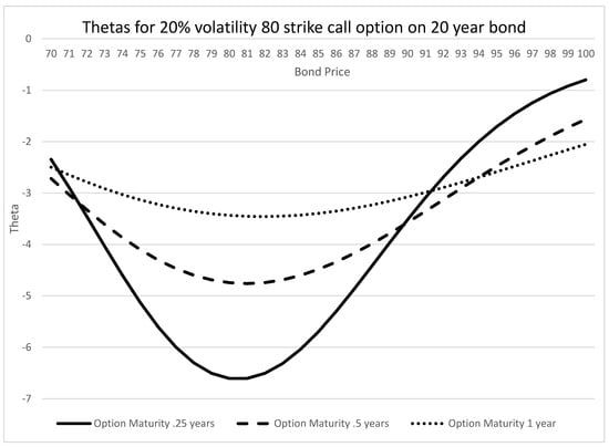
Figure 5. PTP thetas at different option maturities.

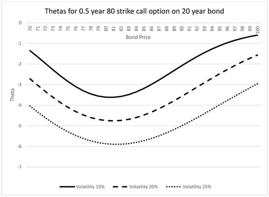
Figure 6. PTP thetas at different volatilities.

The call option’s vega is:

$$\begin{array}{ll}\frac{\partial C}{\partial \sigma }=\frac{B}{\sqrt{2\pi }}{e}^{\left(-\frac{d_1{}^2}{2}\right)}& \left[\left(\frac{1}{2}-\frac{r}{{\sigma }^2}\right)\sqrt{\tau }-\frac{ln\left(\frac{B}{E}\right)}{{\sigma }^2\sqrt{\tau }}\right]+e^{\left(-r\tau \right)}\frac{E}{\sqrt{2\pi }}{e}^{\left(-\frac{d_2{}^2}{2}\right)}\left[\left(\frac{1}{2}+\frac{r}{{\sigma }^2}\right)\sqrt{\tau }+\frac{ln\left(\frac{B}{E}\right)}{{\sigma }^2\sqrt{\tau }}\right]\\ & +\frac{E}{T_B}{e}^{\left(\left(\frac{1}{2}-\frac{r}{{\sigma }^2}\right)ln\left(\frac{B}{E}\right)-\frac{{\left(\sigma +\frac{2r}{\sigma }\right)}^2}{8}\tau \right)}\left\{\right[-\frac{\left(2T_C-\tau \right)\sqrt{\tau }}{2\sqrt{2\pi }}(1+\frac{{\left(ln\left(\frac{B}{E}\right)\right)}^2}{{\sigma }^2\tau }+\frac{2rln\left(\frac{B}{E}\right)}{{\sigma }^2}\\ & -\left({\sigma }^2-{\left(\frac{2r}{\sigma }\right)}^2\right)\frac{\tau }{4}\left)+\frac{{\left(ln\left(\frac{B}{E}\right)\right)}^4-{\left(ln\left(\frac{B}{E}\right)\right)}^2\left|ln\left(\frac{B}{E}\right)\right|}{4{\sigma }^4\sqrt{2\pi \tau }}\right]e^{\left(\raisebox{1ex}{$-{\left(ln\left(\frac{B}{E}\right)\right)}^2$}\!\left/ \!\raisebox{-1ex}{$2{\sigma }^2\tau $}\right.\right)}\\ & +\frac{{\left(ln\left(\frac{B}{E}\right)\right)}^2\left(\left|ln\left(\frac{B}{E}\right)\right|-1\right)}{4{\sigma }^3}\left[\frac{rln\left(\frac{B}{E}\right)}{{\sigma }^2}-\left({\sigma }^2-{\left(\frac{2r}{\sigma }\right)}^2\right)\frac{\tau }{8}-1\right]erfc\left(\frac{\left|ln\left(\frac{B}{E}\right)\right|}{\sigma \sqrt{2\tau }}\right)\}+O\left(\frac{1}{T_B^2}\right)\end{array}$$

Finally, Table 6 presents the vega values for our set of inputs. Not surprisingly, the results mirror those of the other Greeks, with the PTP model values being lower than their Black–Scholes counterparts.

Table 6. Comparison of PTP vegas to Black–Scholes: strike price 80, risk-free rate 0.5%, bond maturity 20 years.

Volatility 15%
	Option Maturity 0.25 Years		Option Maturity 0.5 Years		Option Maturity 1 Year
Bond Price	PTP	Black–Scholes	PTP	Black–Scholes	PTP	Black–Scholes
72	5.3239	5.7688	13.2655	13.3423	24.8610	24.0773
76	12.3032	12.4331	19.7749	19.7351	29.9482	29.5034
80	15.6359	15.9343	22.2208	22.5015	31.7286	31.7286
84	12.9213	13.0714	20.5244	20.5186	30.9206	30.5045
88	6.8675	7.2971	15.3781	15.4301	27.3902	26.6244
Volatility 20%
72	8.5109	8.7884	16.3433	16.3721	27.0008	26.4963
76	13.5092	13.6974	20.5392	20.6476	30.2736	30.0587
80	15.6286	15.9266	22.1999	22.4796	31.6670	31.6670
84	14.1929	14.4005	21.4398	21.5719	31.5097	31.3062
88	10.2028	10.4806	18.5209	18.5645	29.7817	29.2965
Volatility 25%
72	10.4378	10.6743	17.9003	17.9824	27.9662	27.6470
76	14.0918	14.3189	20.8875	21.0651	30.3834	30.2648
80	15.6185	15.9158	22.1708	22.4493	31.5816	31.5816
84	14.8086	15.0538	21.8605	22.0577	31.7404	31.6274
88	12.1349	12.3871	20.0960	20.2053	30.8716	30.5674

Figure 7 and Figure 8 illustrate the thetas for different option maturities and volatilities, respectively.

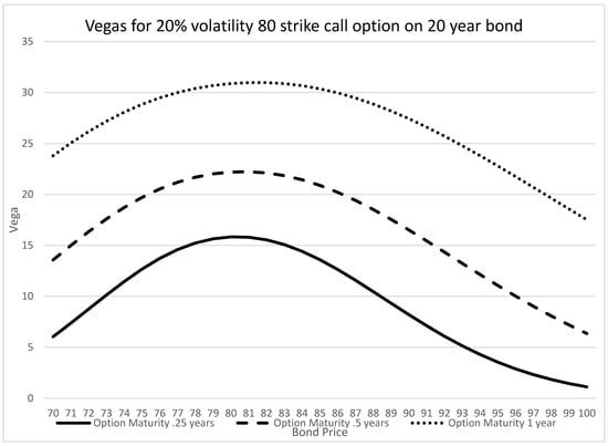
Figure 7. PTP vegas at different option maturities.

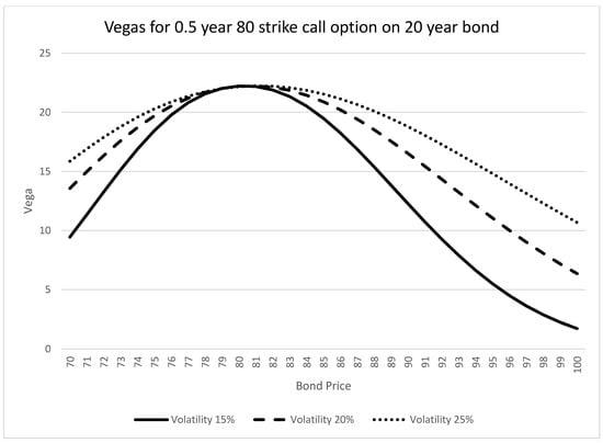
Figure 8. PTP vegas at different volatilities.

6. Conclusions

We derive an asymptotic solution for call options on zero-coupon bonds, assuming a stochastic process for the price of the bond, rather than for interest rates in general. Our approach of modeling bond price dynamics has several important advantages: (1) we are not restricted to assumptions regarding the relationship of interest rates in a term structure; (2) modeling the bond dynamics is computationally simpler than many spot and term structure models with multiple factors; and (3) the resulting solution to our formulation is similar to the familiar Black–Scholes model for European-styled call options on stocks. In our model, we constrain the stochastic process to have a pull-to-par effect and price volatility scales by the remaining original duration of the bond. In this manner, our process more realistically represents the price path of a bond than otherwise given by the geometric Brownian motion proposed in Black and Scholes. The pull-to-par and dampening effect on the volatility results in prices and Greeks that are below those of the Black–Scholes model, in general.

References

- Black, F.; Scholes, M. The Pricing of Options and Corporate Liabilities. J. Political Econ. 1973, 81, 637–654. [Google Scholar] [CrossRef] [Green Version]
- Vasicek, O.A. An Equilibrium Characterization of the Term Structure. J. Financ. Econ. 1977, 5, 177–188. [Google Scholar] [CrossRef]
- Rendleman, R.; Bartter, B. The Pricing of Options on Debt Securities. J. Financ. Quant. Anal. 1980, 15, 11–24. [Google Scholar] [CrossRef]
- Black, F.; Derman, E.; Toy, W. A One-Factor Model of Interest Rates and Its Application to Treasury Bond Options. Financ. Anal. J. 1990, 46, 24–32. [Google Scholar] [CrossRef]
- Black, F.; Karasinski, P. Bond and Option pricing when Short rates are Lognormal. Financ. Anal. J. 1991, 47, 52–59. [Google Scholar] [CrossRef]
- Jamshidian, F. An Exact Bond Option Formula. J. Financ. 1989, 44, 205–209. [Google Scholar] [CrossRef]
- Ho, T.S.; Lee, S. Term Structure Movements and Pricing Interest Rate Contingent Claims. J. Financ. 1986, 41, 1011–1028. [Google Scholar] [CrossRef]
- Heath, D.; Jarrow, R.; Morton, A. Bond Pricing and the Term Structure of Interest Rates: A Discrete Time Approximation. J. Financ. Quant. Anal. 1990, 25, 419–439. [Google Scholar] [CrossRef]
- Heath, D.; Jarrow, R.; Morton, A. Bond Pricing and the Term Structure of Interest Rates: A New Methodology. Econometrica 1992, 60, 77–105. [Google Scholar] [CrossRef]
- Duffie, D.; Kan, R. A Yield-Factor Model of Interest Rates. Math. Financ. 1996, 6, 379–406. [Google Scholar] [CrossRef] [Green Version]
- Brace, A.; Gatarek, D.; Musiela, M. The Market Model of Interest Rate Dynamics. Math. Financ. 1997, 7, 127–154. [Google Scholar] [CrossRef] [Green Version]
- Musiela, M.; Rutkowski, M. Continuous-time term structure models: Forward measure approach. Financ. Stoch. 1997, 1, 261–291. [Google Scholar] [CrossRef] [Green Version]
- Björk, T.; Gaspar, R.M. Interest rate theory and geometry. Port. Math. 2010, 67, 321–367. [Google Scholar] [CrossRef]
- Rebonato, R. Interest-rate term-structure pricing models: A review. Proc. R. Soc. Lond. Ser. A Math. Phys. Eng. Sci. 2004, 460, 667–728. [Google Scholar] [CrossRef]
- Esquível, M.; Gaspar, R.M.; Beleza Sousa, J. Default Propensity Implicit in Pulled to Par VaR for Bonds. Discuss. Math. Probab. Stat. 2017, 37, 79–99. [Google Scholar] [CrossRef] [Green Version]
- Cox, J.C.; Ingersoll, J.E.; Ross, S.A. A Theory of the Term Structure of Interest Rates. Econometrica 1985, 53, 385–407. [Google Scholar] [CrossRef]
- Kevorkian, J.; Cole, J.D. Perturbation Methods in Applied Mathematics. In Applied Mathematical Sciences; John, F., LaSalle, J.P., Sirovich, L., Eds.; Springer: New York, NY, USA, 1981; Volume 34. [Google Scholar]
Publisher’s Note: MDPI stays neutral with regard to jurisdictional claims in published maps and institutional affiliations. |
© 2021 by the authors. Licensee MDPI, Basel, Switzerland. This article is an open access article distributed under the terms and conditions of the Creative Commons Attribution (CC BY) license (https://creativecommons.org/licenses/by/4.0/).