Goodness-of-Fit of Logistic Regression of the Default Rate on GDP Growth Rate and on CDX Indices

Abstract

Under the Basel II and Basel III agreements, the probability of default (PD) is a key parameter used in calculating expected credit loss (ECL), which is typically defined as: PD $\times$ Loss Given Default $\times$ Exposure at Default. In practice or in regulatory requirements, gross domestic product (GDP) has been adopted in the PD estimation model. Due to the problem of excessive fluctuation and highly volatile ECL estimation, models that produce satisfactory PD and thus ECL estimations in the context of existing risk management techniques are lacking. In this study, we explore the usage of the credit default swap index (CDX), a market’s expectation of future PD, as a predictor of the default rate (DR). By comparing the goodness-of-fit of logistic regression, several conclusions are drawn. Firstly, in general, GDP has considerable explanatory power for the default rate which is consistent with current models in practice. Secondly, although both GDP and CDX fit the DR well for rating B class, CDX has a significantly better fit of DR for ratings [A, Baa, Ba]. Thirdly, compared with low-rated companies, the relationship between the DR and GDP is relatively weak for rating A. This phenomenon implies that, in addition to using macroeconomic variables and firm-specific explanatory variables in the PD estimation model, high-rated companies exhibit a greater need to use market supplemental information, such as CDX, to capture the changes in the DR.

1. Introduction

The concept of the probability of default (PD) is generally accepted as the likelihood of a default event over a particular time horizon. Almost all bonds have a credit rating which corresponds to the perceived probability that the issuer will default on its debt repayments [1]. PD value provides an estimate of the likelihood that a borrower will be unable to meet his debt obligations. Under the Basel II and III agreements, the PD is a key parameter used in calculating expected credit loss (ECL) for a bank’s regulatory capital. Starting in 2017, International Financial Reporting Standards 9 (IFRS 9) requires the measurement of impairment loss provisions to be based on an ECL accounting model rather than on an incurred loss accounting model. In fixed income related financial markets, PD forms the essential component for determining stage-wise impairment provisions. Bluhm et al. [2] notes that banks are required to charge an appropriate risk premium for every loan issued. These pooled premiums, called the expected loss reserve in an internal bank account, provide a capital buffer for the possible losses arising from defaults.

1.1. GDP in PD Model

In the Basel Committee on Banking Supervision (BCBS) Consultative Document Guidelines—Guidance on accounting for expected credit losses [3], an effective process which ensures that all relevant information, including forward-looking information and macroeconomic factors such as gross domestic product (annual percent change, GDP), is appropriately considered in assessing and measuring ECL. In practice, GDP growth is generally accepted as a key factor in constructing PD estimation models in both retail and corporate bond markets. In this paper, we focus on corporate bond analytics.

However, in the estimation framework presentation of lifetime PD in accordance with IFRS 9, Đurović [4] records a low effect of the macro-environment on PD development, claiming that this is mainly due to a rapidly changing marketplace and constant increase in the number of market participants. In practice, GDP has been used as a key explanatory variable in estimating PD in the ECL estimation model. However, this approach often leads to dramatic changes in accounting or financial profit and loss due to excessive fluctuations in ECL estimates. This problem was especially abrupt during the financial crisis of 2008 and the COVID-19 pandemic in March 2020.

1.2. Credit Default Swap Index (CDX)

In the analysis of how determinants affect the probability of default, Ortolano and Angelini [5] contend that credit default swap (CDS) is a good indicator of banks’ creditworthiness and an efficient proxy of PD. CDX is a collection of CDS baskets that are completely standardized and exchange-traded; therefore, it is a transparent and liquid measure of synthetic credit risk. The use of liquid CDX spreads allows us to identify the direct credit market influence.

In Exposure Draft ED/2013/3 Financial Instruments [6] issued by IASB, the estimation of ECL of financial instruments, based on the best available information consideration, an entity shall consider information that is reasonably available, including information about past events, current conditions, and reasonable and supportable forecasts of future events and economic conditions. CDX, as a market’s expectation of future PD, should be able to be used as a predictor of the actual DR in the future. D’Amico et al. [7] use the liquid bond exchange-traded fund (ETF) prices and CDX spreads to analyze the influence of the COVID-19 crisis and related Federal Reserve interventions on the underlying corporate bonds. By using market efficient bond ETF prices and CDX spreads, they quantify the impact on the corporate bond market of the 23 March and 9 April 2020 announcements.

1.3. Aims

CDX itself is a proxy of PD, and GDP growth rate represents the growth momentum of the overall economy; both should be able to reflect the changes in DRs in the opposite direction. In this study, we fit annual DRs on GDP and on CDX through a binomial logistic regression model. The main task is not to identify the best statistical model for PD estimation/prediction but to demonstrate how the CDX could significantly outperform GDP growth in fitting historical DRs.

The comparison of the goodness-of-fit between GDP and CDX.IG/HY on the regression of historical DR is motivated by several reasons. First, in practice or regulatory requirements, GDP has been generally adopted in the model for estimating PD, which has become a key factor in the calculation of ECL. Second, ECL estimates exhibited problems of excessive fluctuation and high volatility (e.g., the 2020 COVID-19 pandemic, 2011 European debt crisis, and 2008 financial crisis). Additionally, CDX itself is a timely and efficient proxy of PD that may be integrated into the PD estimation model to improve the ECL estimation.

The main purpose of this study is to build an application base to adopt CDX as one of the key determinants in the PD model in the future. To the best of our knowledge, the CDX index has not been adopted in the ECL (or PD) estimation model so far. This study is the first to explore this topic.

The remainder of this paper is structured as follows. Section 2 presents a literature review on relevant studies. Section 3 describes the basic data property as well as documenting the methodology of the binomial logistic regression model. Section 4 explores the empirical results, and Section 5 discusses the results of this study and other related studies. Finally, Section 6 concludes.

2. Literature Review

Two of the most important regulatory amendments that came about as a result of a series of global financial crises, such as the 2008 Financial Tsunami, are Basel III and IFRS 9. Basel III regulates banks’ capital while IFRS 9 specifies how banks should classify their assets and estimate their future credit losses. Both amendments require the estimation of expected credit losses, which include the PD calculations. One of the main tasks in this study is to explore the goodness-of-fit of the GDP on the realized PD, i.e., the historical DR.

PD models using macroeconomic determinants to study the effects of potential macroeconomic variables, including GDP growth, over credit risk as well as those of regional- or country-level fundamentals or firm-specific variables, are analyzed in many studies (e.g., Koopman and Lucas [8]; Drehmann and Tsatsaronis [9]). Brunel [10] provided a comprehensive survey of PD analytics methodology. To explore the impact of GDP growth on PD, Carvalho et al. [11] observed that with a negative effect on the PD, GDP growth is the most significant among the key macroeconomic predictors of default. However, they also report that reduced PD due to economic growth mostly occurs in economies more exposed to conditions of financial stress. Virolainen [12] studied the macroeconomic determinant variables of Finland Central Bank that affect the credit risk; again, a significant negative relationship between GDP and PD was detected. Castro [13] measured the effect of macroeconomic variables into the banks’ global nonperforming loans, also finding that GDP growth denotes a significant effect on credit risk.

Kırkıl [14] investigated the relationship between the domestic economy and PD and found that GDP is one of the high explanatory variables able to explain PD. By examining the PD in 17 developing countries, Badayi et al. [15] found evidence that suggests macroeconomic variables have a negative impact on PD. The results in Garcia et al. [16] also showed that GDP exerts a considerable influence on banks’ PD. Using 2000–2019 panel data on European commercial banks, results in Jabra [17] indicated that bank default can be explained by GDP. Using data on US loans defaults for 1985–2019, Penikas [18] found evidence that the default correlation may tend to be partially dependent on the GDP growth rate.

Using 22 years of credit ratings data, Pesaran et al. [19] compared the confidence intervals around estimated PD and found that it is impossible to distinguish notch-level PDs for investment-grade ratings. Rho and Saenz [20] found that GDP has a stronger impact on default risk in periods of financial stress versus in tranquil times. They also discovered that financial stress strengthens the impact of GDP on sovereign PD.

Based on the evidence of nonfinancial corporate bond default rates (DRs) over 150 years, Giesecke et al. [21] emphasized the relationship between credit default and the macroeconomic framework. They found that changes in GDP are one of the strong predictors of default rates; however, they also concluded that credit spreads do not adjust in response to realized DR. Conversely, based on data from 40 commercial banks in the Arab region, the results in Obeid [22] show a non-significant statistical impact of GDP on the bankruptcy of the bank. In addition, by using 56 previous empirical studies, Chortareasab et al. [23] performed a meta-analysis on the effect of GDP on nonperforming loans. Their result reveals that the precise effect of GDP performance to credit quality diverges.

3. Data and Methodology

In this study, we analyze the historical DR, which refers to the physical PD, the probability of a real-world default, not the risk-neutral PD which is derived from the valuation concern of a possible default. We explore and compare the goodness-of-fit by regressing the historical DR on GDP and on CDX for various rating classes given default statistics provided by Moody’s [24].

3.1. Data Description

The data contain Moody’s annual issuer-weighted corporate DRs by letter rating. The numbers of observations and DRs by rating class 𝑟 are available. Based on Moody’s default rate metrics, the rating groups which have the same credit rating are determined at the beginning of the year and the default rates are computed over one year. Under Moody’s withdrawal-adjusted default rates, the outstanding number of credits recursively is computed as: $n_t=n_{t-1}-d_{t-1}-w_t$, where $n_t$ is the number of observations, $d_t$ is the number of defaults, and $w_t$ is the withdrawal in period $t$.

The original Moody’s dataset contains corporate default rates by letter rating from 1920 through 2020. Due to economic development and potential structure shifts in the properties of GDP and DR, the sample in this study is restricted to the most recent credits by 𝑡 = 1980, …, 2020 with a total of 41 years of annual data. The reason for the usage of periods 2004–2020 and 2006–2020 is due to the data limitation. The CDX.IG (investment grades for Baa and higher ratings) starts the index from 2004, while CDX.HY (high yield for Ba and lower ratings) starts from 2006. To compare the fitting performance (measured by AIC, and detailed in the Empirical Results section) between CDX and GDP, the same data period for both variables has been used. Additionally, due to the data limitation and to avoid the scarcity of default data in highest-credit entities, the analysis is restricted to rating classes 𝑟 = [𝐴, 𝐵aa, 𝐵a, 𝐵].

The basic information and descriptive statistics for the data are detailed in

Table 1. Basic data information and descriptive statistics.

	$\mathbf{DR}\_\mathbf{A}{ }^1$	DR_Baa	DR_Ba	DR_B	$\mathbf{GDP}-\mathbf{g}\mathbf{r}{ }^2$	$\mathbf{CDX}\_\mathbf{I}\mathbf{G}{ }^3$	CDX_HY 3
Count	41	41	41	41	41	4360	3820
Mean	0.0004	0.0019	0.0093	0.0398	0.0332	78.81	101.12
Std	0.0009	0.0030	0.0111	0.0340	0.0160	35.49	7.56
Min	0.0000	0.0000	0.0000	0.0000	−0.0330	29.03	66.65
25%	0.0000	0.0000	0.0014	0.0106	0.0277	56.41	97.81
(Median)	0.0000	0.0006	0.0051	0.0383	0.0351	68.45	103.04
75%	0.0000	0.0025	0.0139	0.0544	0.0397	93.70	106.79
Max	0.0040	0.0103	0.0384	0.1371	0.0556	279.31	109.99
Skew	2.58	1.87	1.30	1.17	−2.36
Skew_test statistics	4.95	4.06	3.14	2.89	−4.16
p-value	0.0000	0.0001	0.0017	0.0039	0.0000

Data sources: ¹ Moody’s default reports [24]; ² IMF, real GDP growth [26]; ³ Datastream database and Bloomberg.

. It can be seen in Table 1 that the mean default rate of rating A is as low as 0.0004, which is equal to ${{\displaystyle \sum }}_{t=1980}^{2020}{d}_t/{{\displaystyle \sum }}_{t=1980}^{2020}{n}_t=17/41231$. Indeed, this low default scenario has caused serious PD estimation problem which has been discussed extensively in other studies such as in Pluto and Tasche [25]. Figure 1 contains the boxplot of DRs and GDP.

As clearly indicated in the descriptive statistics and the boxplots in the first four columns of Table 1 and Figure 1, the historical DRs of all ratings have a right-skewed distribution. This characteristic can be further verified from the skew statistics and skewness test [27] results in Table 1. All skew test statistics are significantly positive with $p$-values close to zero. The boxplot of the last column in Figure 1 exhibits that GDP is left-skewed distributed with significant negative skew test statistics and close to near-zero $p$-values. Conversely, the DRs of all ratings are right-skewed distributed. This phenomenon corresponds to that of McKinsey’s credit portfolio view model (an econometric model), which assumes an opposite relationship: that an improvement in the macroeconomic factor (such as GDP) will reduce PD.

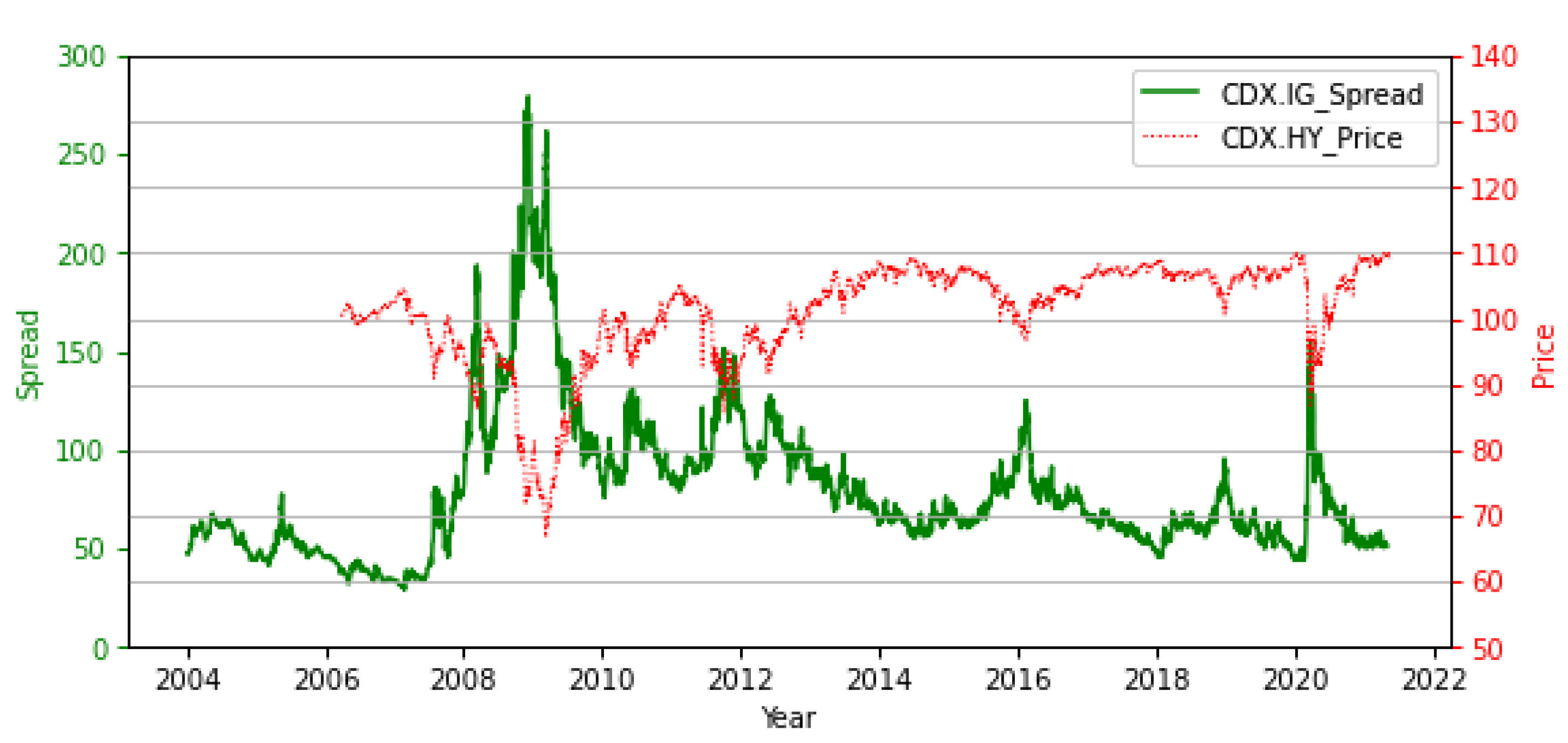
CDX, an exchange-traded instrument with timely data availability, can provide forward-looking information for the overall credit situation. Two of the most liquid CDX indices are the CDX.NA.IG and CDX.NA.HY. Figure 2 contains CDX.IG (since 2004) and CDX.HY (since 2006) daily data.

Figure 2 depicts the reverse trend between CDX.IG and CDX.HY. Conventionally, high-yield CDS indices are quoted in prices, unlike their investment-grade equivalents, which are quoted in spread basis points (bps). A high-yield CDS index with a zero net-present value will be quoted as having a price of 100. This difference in quotation convention reflects that buying a high-yield CDS index involves “long risk,” whereas buying an investment-grade index or any single-name CDS contract involves “long protection” and “short risk”. A rough formula for the relationship between the price and the spread is spread = coupon + 100 × (100 − price)/tenor. For instance, if the CDX.HY is quoted as 103 (close to the median in the data), the coupon is 500 bps, and the tenor is 5 years, then the spread is 500 + (−300)/5 = 440 bps.

We fit the DRs of investment rating classes [A, Baa] on the CDX.IG index and fit the DRs of noninvestment ratings [Ba, B] on the CDX.HY index. As a market indicator, the CDX index is considered highly volatile. For demonstrative purposes, we use the CDX annual average to fit Moody’s annual DRs. Additionally, to be consistent with the historical DRs in the comparison, the average daily CDX and year-end adjusted GDP for the past year—both realized and historical data—are used in this study.

3.2. Methodology

In this paper, we are mainly concerned with the relationship of historical DR with GDP and CDX data. We use a logistic regression model with binominal data to fit pooled historical default rates. The definition of default is in Basel II (BCBS 2006, paragraph 452) [28] and Basel III (BCBS 2017, paragraph 220) [29]: a default is considered to have occurred with regard to a particular obligor when either or both of the two following events have taken place:

• The bank considers that the obligor is unlikely to pay its credit obligations to the banking group in full, without recourse by the bank to actions such as realizing security (if held);
• The obligor is past due more than 90 days on any material credit obligation to the banking group and will be considered as being past due once the customer has breached an advised limit or been advised of a limit smaller than current outstandings.

In a more general and intuitive sense, the PD can be broadly defined as the probability of either or both events in the Basel definition being realized. Given a binary outcome variable (i.e., a variable with only two possible outcomes, 0 [no default] or 1 [default]) $L$ and a set of explanatory variables $\mathit{x}$. The basic setup of the logistic regression model is as follows: conditional on $\mathit{x}$, the outcome variable $L$ is described as Bernoulli distributed; that is, $L|\mathit{x} ~$Bernoulli distributed ($p$) for some $p\in \left[0,1\right]$. The goal of logistic regression is to create a predictive model for the binary outcome variable.

In logistic regression, the logarithm of the odds is the logit of the probability. The logit of the probability $p$ is defined as

$$\mathrm{logit} p=\ln \frac{p}{1-p}, \mathrm{for} 0<p<1$$

(1)

and the logit link function is defined as

$$\mathrm{logit} \mathrm{E}(L|\mathit{x})={\mathit{\beta }}^{\prime }\mathit{x}$$

(2)

where $L$ is the binary outcome variable and $\mathit{x}$ is the explanatory variables; $\mathit{\beta }$ represents the linear parameters. Although the dependent variable in logistic regression is Bernoulli distributed, the logit is on an unrestricted scale. The logit function is the link function in this type of generalized linear model. Let the random variable $L_{i,t}$ be defined as

$$L_{i,t}=\{\begin{array}{c}1, \mathrm{t}\mathrm{h}\mathrm{e} i^{\mathrm{th}} \mathrm{L}\mathrm{o}\mathrm{a}\mathrm{n} \mathrm{o}\mathrm{f} t^{\mathrm{th}} \mathrm{y}\mathrm{e}\mathrm{a}\mathrm{r} \mathrm{i}\mathrm{s} \mathrm{i}\mathrm{n} \mathrm{t}\mathrm{h}\mathrm{e} \mathrm{e}\mathrm{v}\mathrm{e}\mathrm{n}\mathrm{t} \mathrm{o}\mathrm{f} \mathrm{d}\mathrm{e}\mathrm{f}\mathrm{a}\mathrm{u}\mathrm{l}\mathrm{t} \\ 0, \mathrm{t}\mathrm{h}\mathrm{e} i^{\mathrm{th}} \mathrm{L}\mathrm{o}\mathrm{a}\mathrm{n} \mathrm{o}\mathrm{f} t^{\mathrm{th}} \mathrm{y}\mathrm{e}\mathrm{a}\mathrm{r}\mathrm{ }\mathrm{i}\mathrm{s} \mathrm{i}\mathrm{n} \mathrm{t}\mathrm{h}\mathrm{e} \mathrm{e}\mathrm{v}\mathrm{e}\mathrm{n}\mathrm{t} \mathrm{o}\mathrm{f} \mathrm{n}\mathrm{o} \mathrm{d}\mathrm{e}\mathrm{f}\mathrm{a}\mathrm{u}\mathrm{l}\mathrm{t}\end{array}$$

(3)

and the PD for a rating class in the same year is assumed to be constant. Thus, conditional on a set of predictor variables ${\mathit{x}}_t$, the random variable $L_{i,t}$ is a Bernoulli random variable with

$$P\left(L_{i,t}=1|{\mathit{x}}_t\right)=P\left(\mathrm{Default}\right)=p_t=\mathrm{PD}$$

(4)

and

$$P\left(L_{i,t}=0|x_t\right)=P\left(\mathrm{NonDefault}\right)=1-p_t=P\left(\mathrm{Survival}\right)$$

(5)

Given this definition, the Bernoulli distribution is an intuitive model for determining the defaults [2]. Hence, the observation of $n_t$ credit exposures can be written as

$${\mathit{L}}_t\equiv \left(L_{1,t}, \cdots ,L_{i,t},\cdots ,L_{n_t,t}\right)\mathrm{with}{L}_{i,t}|x_t~\mathrm{Bernoulli}\left(1;p_t\right), i=1,\cdots , n_t.$$

(6)

In terms of binomial data, the random variables $L_{1,t}, \cdots ,L_{i,t},\cdots ,L_{n_t,t}$ are assumed to be independent and $Y_t$ is defined as

$$Y_t\equiv L_{1,t}+L_{2,t}+\cdots +L_{n_t,t}$$

(7)

Because $L_{1,t}, \cdots ,L_{i,t},\cdots ,L_{n_t,t}$ are $n_t$ independent and identically distributed trials, $Y_t$ is the number of defaults observed (the sum of the individual Bernoulli distributed random variables) and hence, conditional on ${\mathit{x}}_t$, $Y_t$ follows a binomial distribution as

$$Y_t|{\mathit{x}}_t~\mathrm{binomial}\left(n_t;p_t\right), t=1,\cdots , T,$$

(8)

where $T$ is the number of years for the default data. In terms of expected values,

$$\mathrm{E}(\frac{Y_t}{n_t}|{\mathit{x}}_t)=p_t$$

(9)

then

$$\mathrm{logit} \left(\mathrm{E}(\frac{Y_t}{n_t}|x_t)\right)=\mathrm{logit}\left(p_t\right)=\ln \frac{p_t}{1-p_t}={\mathit{\beta }}^{\prime }{\mathit{x}}_t,$$

(10)

$$P\left(Y_t=y|{\mathit{x}}_t;\mathit{\beta }\right)=\left(\begin{array}{c}{n}_t\\ y\end{array}\right)p_t^y{\left(1-p_t\right)}^{n_t-y}=\left(\begin{array}{c}{n}_t\\ y\end{array}\right){\left(\frac{1}{1+{\mathrm{e}}^{-{\mathit{\beta }}^{\prime }{\mathit{x}}_t}}\right)}^{\mathrm{y}}{\left(1-\frac{1}{1+{\mathrm{e}}^{-{\mathit{\beta }}^{\prime }{\mathit{x}}_t}}\right)}^{n_t-\mathrm{y}}$$

(11)

The likelihood function, assuming that all the observations $\left(Y_1,Y_2,\cdots ,Y_T\right)$ are independently binomial distributed, is defined as

$$Lik\left(\mathit{\beta }|\mathit{y};\mathit{x}\right)={{\displaystyle \prod }}_{t=1}^{T}P\left(y_t|{\mathit{x}}_t;\mathit{\beta }\right)$$

(12)

Generally, the log-likelihood function defined as

$$\ell \left(\mathit{\beta }|\mathit{y};\mathit{x}\right)\equiv \log Lik\left(\mathit{\beta }|\mathit{y};\mathit{x}\right)={{\displaystyle \sum }}_{t=1}^{T}P\left(y_t|{\mathit{x}}_t;\mathit{\beta }\right)$$

(13)

is maximized using various optimization techniques, such as the gradient descent method. The “statsmodels” [30] package in Python to implement the logistic regression model (under a generalized linear model) is used in this empirical study.

4. Empirical Results

Figure 3, Figure 4, Figure 5 and Figure 6 exhibit the results of the binomial logistic regression of ratings A, Baa, Ba, and B, respectively. Correspondingly,

Table 2. Rating A: model parameter estimates and $p$-values.

(a)	Coef	Std Err	Test	$$\mathit{p}$$
Const	−7.223	0.359	−20.094	0.000
GDP (1980–)	−19.436	10.176	−1.910	0.056
(b)	Coef	Std Err	Test	$p$
Const	−7.134	0.409	−17.423	0.000
GDP (2004–)	−12.094	10.610	−1.140	0.254
(c)	Coef	Std Err	Test	$p$
Const	−11.550	1.222	−9.448	0.000
CDX.IG	0.039	0.009	4.184	0.000

,

Table 3. Rating Baa: model parameter estimates and $p$-values.

(a)	Coef	Std Err	Test	$\mathit{p}$
Const	−5.895	0.175	−33.723	0.000
GDP (1980–)	−14.586	4.840	−3.014	0.003
(b)	Coef	Std Err	Test	$p$
Const	−5.971	0.192	−31.041	0.000
GDP (2004–)	−16.988	5.192	−3.272	0.001
(c)	Coef	Std Err	Test	$p$
Const	−10.214	0.602	−16.965	0.000
CDX.IG	0.038	0.005	7.969	0.000

,

Table 4. Rating Ba: model parameter estimates and $p$-values.

(a)	Coef	Std Err	Test	$\mathit{p}$
Const	−4.601	0.144	−31.897	0.000
GDP (1980–)	−6.306	3.930	−1.604	0.109
(b)	Coef	Std Err	Z	p > |z|
Const	−5.169	0.202	−25.585	0.000
GDP (2006–)	−12.895	5.559	−2.320	0.020
(c)	Coef	Std Err	Test	$p$
Const	7.150	1.773	4.033	0.000
CDX.HY	−0.130	0.019	−6.881	0.000

and

Table 5. Rating B: model parameter estimates and $p$-values.

(a)	Coef	Std Err	Test	$\mathit{p}$
Const	−2.933	0.057	−51.740	0.000
GDP (1980–)	−15.247	1.534	−9.940	0.000
(b)	Coef	Std Err	Test	$p$
Const	−3.493	0.074	−47.197	0.000
GDP (2006–)	−24.128	2.095	−11.516	0.000
(c)	Coef	Std Err	Test	$p$
Const	4.325	0.797	5.426	0.000
CDX.HY	−0.085	0.008	−10.381	0.000

display the goodness-of-fit parameter estimates and p values for each rate. Starting from the probability density function in Equation (11), the maximum likelihood estimation (MLE) and the associated Akaike information criterion (AIC) were used in selecting the best fitted logistic regression model with optimal parameters for the historical DRs. The results are obtained by MLE and using the expectation-maximization algorithm [31] implemented in the “statsmodels” fitting procedure in Python. The model parameter estimates and $p$ values are listed in Table 2, Table 3, Table 4 and Table 5, corresponding to ratings A, Baa, Ba, and B, respectively. Under the null hypothesis $H_0,$ the logistic regression model does not provide a better fit to the data than a model that contains no explanatory variable. Equivalently as $H_0,$ the logistic regression coefficient is equal to zero, and the $p$-value, defined as $p=P\left(\mathrm{reject} H_0|H_0\right)$, is a measure of evidence against the null hypothesis that the coefficient is zero, or the goodness-of-fit is inadequate.

The fit results of rating A are displayed in Figure 3 and Table 2, which indicate that using 1980–2020 data (upper left with $p$-value = 0.056) has a better fit than using 2004–2020 data does (lower left with $p$-value = 0.254). This phenomenon may be attributable to the fact that defaults in rating A are few and the use of more years of data can reduce some bias due to data scarcity. Notably, the estimated GDP coefficient is negative (−19.436 and −12.094 for the 1980–2020 and 2004–2020 data sets, respectively) whereas that of CDX.IG (in spread) is positive (0.039). This is due to a negative relationship between DR and GDP as well as a positive relationship between DR and CDX.IG spread.

For rating Baa, Figure 4 and Table 3 indicate that GDP in both the 1980–2020 and 2004–2020 data sets can fit DR well (with $p$-values = 0.003 and 0.001, respectively). In addition, CDX.IG can fit even better with a $p$-value < 0.001.

For rating Ba, Figure 5 and Table 4 show that using 1980–2020 data (panel (a) with $p$-value = 0.109) achieves an inferior fit to that obtained using 2006–2020 data (panel (b) with $p$-value = 0.020). Nevertheless, the CDX.HY $p$-value (close to zero) in panel (c) indicates an optimal fit. As a sub-conclusion, Figure 3, Figure 4 and Figure 5 indicate that the fit results of DR on CDX (panel (c)) are far superior to those of GDP (panels (a) and (b)) for ratings A, Baa, and Ba, respectively. This phenomenon can also be ascertained from the $p$-values in Table 2, Table 3 and Table 4. Notably, both the estimated GDP and CDX.HY (in price) coefficients are negative. This is because DR has a negative relationship with GDP and CDX.HY. The reverse relationship between CDX.IG (in spread) and CDX.HY (in price) is described in the Data and Methodology section.

Compared with higher-rated companies, those with the B rating exhibit a special phenomenon: GDP is markedly well-fitted to DR. Figure 6 and Table 5 suggest that both GDP and CDX.HY fit DR well for rating B. All tests yield $p$-values close to zero. Specifically, the GDP performs even better than CDX.HY when the 2006–2020 data set is used in the fit of DR. This phenomenon can be explained by the fact that the real economy (GDP, macroeconomics) is more directly connected to the defaults of lower-rated companies. When the macroeconomy declines, its influence will be more quickly linked to those companies’ DRs compared with higher-rated companies.

In summary, except for rating B, the fitness of DR on CDX outperforms that on GDP. This result can be further verified from the AIC results shown in

Table 6. AIC of Goodness-of-Fit: regression of DR on GDP and on CDX.IG/HY.

Ratings	Data Period	AIC of GDP	AIC of CDX.IG/HY
A	2004~2020	49.925	28.655
Baa	2004~2020	114.780	52.556
Ba	2006~2020	107.572	67.758
B	2006~2020	202.337	215.049

. The aforementioned AIC can be used to assess the fitness of a statistical model and is defined as

$$\mathrm{AIC}=2k-2\log \widehat{Lik}\left(·\right)$$

(14)

where $k$ is the number of model parameters ($k$= 1, in this study) and $\log \widehat{Lik}\left(·\right)$ is the maximum value of the log-likelihood function in Equation (13); due to its property of penalty function, the smaller AIC value suggests a better fit. Thus, the smaller the AIC value, the better the model fit is. Note that because the number of years of data (sample size) used will affect the calculation of the likelihood function value and the AIC estimate, Table 6 only lists the AIC with the same data period for each rating.

Table 6 suggests that all AICs of CDX for ratings [A, Baa, Ba] are smaller and therefore superior. For rating B, when the same data period (2006–2020) is used, the AIC of GDP is smaller than that of CDX.HY (202.337 vs. 215.049) which indicates that GDP has a better fit to DR (compared with CDX.HY).

The aforementioned empirical analysis indicates that, for high-rated (e.g., rating A) companies, the relationship between DR and GDP is relatively weak, a fact which may be related to default data scarcity. Another possible reason is that one of the main criteria in ratings for high-rated companies is cyclical neutral; hence, the operation of high-rated companies should be minimally affected by the overall business cycle. In other words, the basic rating philosophy assumes that the DR of a high-rated company is not strongly correlated with macroeconomic factors, such as GDP.

Regardless of the reason, this phenomenon highlights an important practical point: compared with low-rated companies, in addition to using macro variables such as GDP and firm-specific explanatory variables in their PD estimation model, high-rated companies have a greater need for supplemental information (e.g., market trade data such as CDX) to capture the changes in DR in an effective and timely manner to meet regulatory requirements and practical needs. This result may echo the guidelines on credit institutions’ credit risk management practices and accounting for expected credit losses [32], which state that “where market indicators (such as CDS spreads) are available, senior management may consider them to be a valid benchmark against which to check the consistency of its own judgements.”

5. Discussion

Empirical fitted results of DR in this study show that, except for rating B, market credit index (CDX) outperforms economic factor (GDP) significantly. This result is consistent with that of Ortolano and Angelini [5]. However, it is in contrast to Giesecke et al. [21] who concluded that GDP is a strong predictor of default rates and that credit spreads do not adjust well in response to realized DR. One possible reason for this phenomenon is that when market-traded credit instruments (such as CDX) become more complete, the credit indicators traded in the market will have a stronger correlation with the default rate compared to corporate bond spread used in [21]. In contrast, with the effects of market intervention policies such as QE and low (or even negative) interest rates, the link between economic indicators (such as GDP) and default rates may gradually weaken over time. This phenomenon may also become more obvious due to the occurrence of COVID-19.

In Section 4, the default rates are regressed on either the GDP growth rates or a CDS index. The aforementioned empirical results show that CDX.IG/HY significantly outperforms GDP in the cases of A, Baa, and Ba ratings, and that both GDP and CDX are almost equally significant for rating B. In fact, the default rates have also been regressed on both the GDP growth rates and a CDS index together in this study. Here, we call it the ‘full’ model. As expected, the GDP variable shows no significant effect in the full model for ratings A, Baa, and Ba, while GDP and CDX are both significant in the full model for rating B. This is not a surprising result. Since the main purpose in this study is to demonstrate the potential usage of CDX in the PD model, the resulting figures and tables of the full model are not listed here.

6. Conclusions

In response to a lack of models that produce satisfactory PD and thus ECL estimation in the context of existing risk management techniques, this paper is drafted to link PD to different rating classes and complies with IFRS accounting standards. Several conclusions are drawn from this paper. First, in general, a considerable inverse relationship between GDP and DR is observed. In other words, GDP has substantial explanatory power for DR. This result is consistent with GDP usually being adopted as a key factor in PD estimation models in academia or in practical usage (e.g., the credit portfolio view model). Second, the primary link between historical DR and CDX for both IG and HY is confirmed. Third, in the logistic regression model of DR, although both GDP and CDX.IG/HY fit DR well for rating B, using CDX.IG/HY to fit DR produces a significantly better fit than using GDP for ratings A, Baa, and Ba. Lastly, and most importantly, the relationship between DR and GDP is relatively weak for high-rated (e.g., rating A) companies. This implies that, compared with low-rated companies, in addition to using macro variables and firm-specific explanatory variables in PD estimation models, high-rated companies have a greater need to use supplemental information (such as CDX) to capture the changes in DR and meet regulatory requirements and practical needs.

A limitation in this study is that the data for the quarterly/monthly GDP and historical default rates are not available. Only annual data were used in this study. One of the potential future research directions is to replace GDP with CDX.IG/HY in the PD model and see if the new model increases PD predictability significantly.