Abstract
We propose a new multi-moment numerical solver for hyperbolic conservation laws by using the alternating polynomial reconstruction approach. Unlike existing multi-moment schemes, our approach updates model variables by implementing two polynomial reconstructions alternately. First, Hermite interpolation reconstructs the solution within the cell by matching the point-based variables containing both physical values and their spatial derivatives. Then the reconstructed solution is updated by the Euler method. Second, we solve a constrained least-squares problem to correct the updated solution to preserve the conservation laws. Our method enjoys the advantages of a compact numerical stencil and high-order accuracy. Fourier analysis also indicates that our method allows a larger CFL number compared with many other high-order schemes. By adding a proper amount of artificial viscosity, shock waves and other discontinuities can also be computed accurately and sharply without solving an approximated Riemann problem.
1. Introduction
In this paper, we aim to solve the hyperbolic conservation law
where u and can be either scalars or vectors.
The classical higher-order numerical schemes such as the finite difference (FD) and the finite volume (FV) frameworks usually involve only one degree of freedom (DOF) per cell. That means to achieve the kth order discretization of the first-order spatial derivative, a stencil of at least cells is required. The compactness of a scheme can help simplify the polynomial interpolation in unstructured meshes and reduce communication costs between computational nodes on modern supercomputers. In this paper, the “compact” is used specifically for numerical schemes with a minimal stencil, which excludes so-called Padê schemes [1,2] since its approximation of the derivative involves solving a diagonal system of the full difference stencil.
A natural thought for the design of a compact high-order scheme is involving more than one DOF per cell so as to construct higher-order polynomials under the same stencil width. A series of multi-moment schemes is developed based on this idea. The constrained interpolation profile (CIP) scheme [3,4], which uses the semi-Lagrangian method to advance in time, individually updates the physical variable and its derivatives on each cell by the governing equations in different forms. The interpolated differential operator (IDO) method [5] is similar to CIP but uses an explicit time-advancing approach. For the IDO method, a stencil containing three adjacent cells suffices to approximate the first-order spatial derivative with fifth-order accuracy in one dimension, which makes it possible to obtain comparably accurate results with spectral methods in direct numerical simulation [6]. For IDO, updating the derivative-value variables induces the problem of computing the time derivative of , which involves . However, for the system of conservation laws, has a fairly complicated form and can be difficult to compute. Goodrich et al. proposed a similar Hermite method [7] on staggered grids.
Neither CIP nor IDO are conservative schemes, which means they are not ideal for shock-capturing problems and long-term simulations. To address the non-conservativeness, so-called CIP-conservative semi-Lagrangian (CIP-CSL) schemes [8,9] and the IDO scheme in conservative form (IDO-CF) [10,11] add the cell-averaged value as an extra independent model variable to evolve. The cell-averaged variable is advanced by the flux-form conservation law and is hence exactly conserved, while other kinds of variables are updated using the differential form of conservation laws. However, these conservative CIP algorithms need to find polynomials that match cell-averaged variables across cells, which can be time-consuming when encountered with non-uniform meshes. A framework termed the multi-moment finite volume method (MM-FVM) has been proposed on the basis of CIP-CSL. Compared with CIP-CSL, MM-FVM can construct the high-order interpolation on a local base and is more flexible when treating unstructured grids, as shown in [12]. Nonetheless, MM-FVM uses the semi-Lagrangian method in the time integration of point-based variables, which is difficult to implement in the multi-dimensional case.
Another class of high-order conservative schemes based on local flux reconstructions also uses a compact stencil and has become increasingly attractive in recent decades. Examples include the well-known discontinuous Galerkin (DG) [13,14,15], spectral volume [16,17], and spectral difference [18] methods and, more recently, the flux reconstruction/correction via procedure (FR/CPR) method [19,20]. These methods evolve k DOFs in each cell for a kth order spatial accuracy (in one dimension) and compute the numerical flux on cell boundaries to represent the interaction between adjacent cells. Thus, polynomial interpolation across cells is not needed, which makes these methods compact and flexible in handling unstructured meshes. The multi-moment constrained finite volume (MCV) method proposed by Ii and Xiao [21] can be viewed as a combination of CIP and the flux reconstruction approach. The MCV method introduces high-order spatial derivatives of numerical flux and reconstructs the local flux function more directly. MCV is generalized as multi-moment constrained flux reconstruction (MMC-FR) [22]. However, the nonlinear aliasing phenomenon [23,24] in treating nonlinear flux functions, which causes instability and accuracy loss, is one typical demerit for these methods based on local flux reconstruction.
This paper presents a novel conservative multi-moment approach termed the AltPoly method, which uses the alternating polynomial reconstruction as the time integration method. AltPoly divides the computational domain into cells and adopts point-based and cell-averaged values as model variables. The point-based variables including the physical variable and its spatial derivatives are updated together, which is different from the conventional multi-moment methods that update different types of model variables according to governing equations in different forms. AltPoly then solves a constrained least-squares problem to reconstruct the solution within the cell and update the model variables, which preserves conservativeness exactly. Solving Riemann problems on cell boundaries is not needed. Furthermore, AltPoly can also handle non-uniform meshes in one dimension efficiently with the aid of the coordinate transform.
The remainder of this paper is organized as follows: Section 2 describes the formulation of AltPoly and constructs artificial viscosity for discontinuous problems. Section 3 studies the accuracy and stability of AltPoly by Fourier analysis. Section 4 validates the numerical convergence rate and capability of solving some widely used benchmark problems involving both the scalar equation and Euler systems in 1D. Finally, a short summary in Section 5 ends this paper.
2. Formulation of AltPoly Method
This section gives the formulation of the AltPoly method for a one-dimensional conservation law. For concreteness and ease of comprehension, we only present the detailed formulation for AltPoly with 2 point-value variables and one extra cell-averaged variable per cell, which is termed AltPoly-3. As for the general AltPoly-r with r model variables within a cell, the formulation is similar to AltPoly-3 and is hence briefly illustrated in Appendix A.
To begin with, we first introduce some notation. The bold font lower-case letter denotes a column vector, e.g., . The transpose is denoted by . denotes the kth standard unit vector in a space in proper dimensions. denotes a column vector in the form of . Bold font capital letters such as denote matrices. The submatrix of constructed from rows and columns is denoted as . denotes the 2-norm of the vector , while for a matrix is defined by
2.1. Spatial Discretization and Model Variables
Suppose the spatial domain is divided into N non-overlapping cells, among which the j-th cell is , . It should be noted that the cells do not necessarily have a uniform length. In the j-th element, we consider computing the time integration of three model variables: , at the middle point of the element, and additionally the element-integrated value .
2.2. Updating Model Variables
Denote the model variables at time level as . This part illustrates the procedure to obtain with , where is the time step length. In a nutshell, this procedure consists of 3 steps:
- Hermite interpolation across cells using point-based variables;
- Computing solution values on selected solution points based on reconstructed polynomials and updating solution values and cell-averaged variables via the Euler forward method;
- Reconstructing the solution polynomial that matches updated solution values under the constraint of cell-averaged variables to preserve conservativeness.
Details are presented in the following and algorithm illustrations are presented in Figure 1 for convenience of illustration.
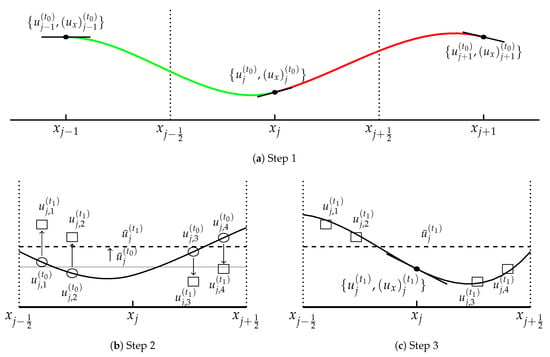
Figure 1.
Algorithm illustration.
2.2.1. Step 1: Hermite Interpolation across Cells
In the first step, we find the interpolation polynomial on the interval that matches as shown in Figure 1a. This step does not involve cell-averaged variables . This interpolation polynomial is of the third order since there are 4 conditions in total. Before constructing , we introduce a local coordinate
for as is usually done in the finite element method [25]. The local coordinate can unify the interpolation templates so as to reduce the computational cost. The polynomial on the local coordinate s is denoted by . Notice that and can be connected by the following rule:
Then the coefficients of can be determined by the following system:
The matrix form is
where
In practice, the inverse of is computed and stored in advance so as to reduce the computation cost in solving (4).
2.2.2. Step 2: Updating Solution Values on Solution Points
Based on Step 1, we can now approximate and update the solution in cell using polynomials and . For AltPoly-3, four symmetric solution points on are needed in this step with . In this paper, we choose and as solution points with . To update the solution values on these solution points, we need to compute
to approximate u and . For convenience, we transfer the solution points into local coordinate for . Combining the conservative law (1) we can then compute by the Euler forward method:
where the function stands for .
The cell-averaged variable is updated by the flux form of the conservation law:
where is the function value at the cell boundary computed by
When the computing grid is uniform, (10) is simply
Figure 1b describes this step.
Remark 1.
The Euler time integration used for updating solution values on solution points is simple and easy to implement. However, the semi-Lagrangian time integration scheme [26] might be robust with a larger time step.
2.2.3. Step 3: Updating Model Variables
The cell-averaged variable has been updated (9). As for the point-value model variables, the four updated solution values on suffice to reconstruct a Lagrange interpolation polynomial , so as to obtain the updated model variables and . However, such a direct routine may cause the mismatch of and .
Similar to Step 1, we introduce a local coordinate :
Let be under the local coordinate . Then all conditions for are listed as
This is an over-determined linear system since it contains 5 conditions and 4 unknowns. However, (13) must hold for ensuring the conservation law. In other words, we need to find the optimal coefficients to fit (12) under the constraint (13). This is a typical constrained least-squares problem. To solve this, we rewrite the constraint (13) as
and plug it into (12). Then the constrained least-squares problem is cast into the standard least-squares problem as
where
Then the solution of (15) is
where is the generalized inverse or the Moore–Penrose inverse [27] of non-square matrix .
From the polynomial expression of , we can now retrieve the point-value model variables for the next time level:
This polynomial reconstruction of based on solving constrained squares problem (13) can be efficiently implemented if we compute and store in advance.
2.3. Runge–Kutta Time Integration
Up to this point, we have only presented AltPoly using the Euler forward method, which is merely of first-order temporal accuracy. Since the presented AltPoly is not in the semi-discretization form, the Runge–Kutta algorithm cannot be directly applied for AltPoly. Therefore, a slight modification of the Runge–Kutta algorithm is adopted here.
To proceed, we introduce the following notation. Let be a compounded list of all model variables, and its j-th entry is a vector . Denote the result of AltPoly upon after one step with length of the temporal forward Euler method by and the corresponding increment part is denoted by
Then, one time step of the Runge–Kutta procedure for AltPoly is
where
2.4. Artificial Viscosity
To tackle problems that involve discontinuities such as shocks and contact discontinuities, we add artificial viscosities to the proposed method. The critical step is depicting the smoothness of a cell and determining whether the discontinuity exists. Our shock sensor borrows the idea from the sub-cell shock capturing for DG [28].
Within each cell, we define the following truncated cell average based on the moments for AltPoly-r:
where is the largest even number smaller than r. It can be seen that utilizes the even-order partial differential point-value moments and is an approximation of with the error of magnitude . Therefore, we expect that the solution is continuous and then is close enough to , and hence declaim that a discontinuity exists in if exceeds some threshold. Based on this, the following smoothness indicator is defined:
where and the parameter is added to avoid dividing zero. This smoothness indicator has a simple form and can be calculated directly from the model variables. Then the amount of viscosity at is calculated by the following smooth function,
where , the parameters , , and is large enough to maintain a sharp but smooth shock profile.
So far, we have obtained the viscosity at the middle of each cell. Next we use the linear interpolation to construct the viscosity function between the middle points of two adjacent cells. Then, to solve the problem with this viscosity function, one only needs to replace with , and modify (8) and (9), respectively.
3. Fourier (von Neumann) Analysis
This part gives the Fourier analyses of stability and accuracy for AltPoly in solving a linear advection equation. We only give a detailed analysis for AltPoly-3 for concreteness. AltPoly-r with other choices of r can be analyzed following a similar routine.
3.1. Formulation of the Amplification Matrix
Consider the linear scalar equation
Suppose the computational domain is with a uniform mesh spacing . The initial condition is periodic: where denotes the imaginary unit, and is the scaled wavenumber. The initial values of model variables on the cell and its neighbor cells are given by
The discrete Fourier transform of the series is
is not 0 only when under the given initial condition. Hence, we only need to consider the Fourier coefficient and denote it as in the following text for simplicity. and are defined similarly for series and
The key procedure in our analysis is rewriting the AltPoly-3 formulation in Section 2 into the matrix form:
where is defined as , and denotes the amplification matrix connecting at the next time level
The coefficient vector of the reconstructed polynomial in Step 1 of AltPoly-3 is
where ,
According to (26), we have and according to the periodicity of the spatial profile. According to (10), the function values at the cell boundaries are
where denotes the k-th standard unit vector.
Now we turn to Step 2 of AltPoly-3. As the solution points and are in the domain of , we transfer them into the local coordinate in . Let and . Then we can derive
Similarly, the variable value and first spatial derivatives on solution points can be computed by
where and .
Combining , the updating of solution values on solution points can be expressed in the following matrix form:
where the items of , are, respectively:
with defined as 1, and is a diagonal matrix with on the diagonal line.
Since , the updated solution values here are computed by
where the CFL number for this linear problem.
As for Step 3, the updated cell average over the jth cell is
Solving a constrained least-squares problem we have
From we can easily obtain point-value variables of the next time level:
3.2. Accuracy Analysis
At the beginning, we assumed AltPoly-3 only had third-order spatial accuracy since all reconstruction polynomials are of the fourth-order, which has third-order spatial accuracy for first-order derivatives. Instead, however, we observed fourth-order spatial accuracy in numerical tests. Analyzing only truncation error is not enough to explain this phenomenon. We believe that the cell-averaged moment and the constrained polynomial reconstruction help improve the spatial accuracy.
The amplification matrix can be divided into two parts,
where and are independent from c. Let . The principal eigenvalue of is 1 (see Appendix B for details). We denote the corresponding eigenvector as , namely
and we make the last items of and equal, namely .
With the assistance of Wolfram Mathematica 12, we decompose the following terms into Taylor series
and
where the scalars and the vectors are independent with w.
Suppose we choose a proper c that ensures the stability, namely for and some positive constant M. Divide the time domain uniformly with step length and denote . It is obvious that the exact solution at for (53) with the initial condition is . Hence the error of the numerical solution by AltPoly-3 is
However,
According to the bound result (A16) in Appendix B, with some positive constants Then one can deduce that
Remember that , and then we have
Combining (44)–(47), we can see that the error order of AltPoly-3 is
To ensure stability, the order of magnitude of is usually not higher than that of , namely . Therefore, the truncated error (48) can be simply reduced to That means AltPoly-3 using the Euler time scheme has fourth-order spatial accuracy and first-order temporal accuracy.
When using RK4 as time integration strategy (20), the amplification matrix for this linear equation can be expressed as
where
Expanding , we have
One can easily show that has fifth-order truncated temporal accuracy and then the total error becomes
3.3. Stability Analysis
To obtain stable time integration, the CFL number c should be carefully chosen such that the magnitude of the principal eigenvalue of the amplification matrix is not greater than 1 for all wavenumbers k. The principal eigenvalue of the amplification matrix for AltPoly with various moments can be seen in Figure 2. It is remarkable that all schemes have a fairly large range of c except for AltPoly-5. In particular, AltPoly-3, which has fourth-order spatial accuracy, is stable even with , which is better than many other existing explicit high-order schemes using a compact stencil. As more moments are used, the stability condition becomes more stringent. For AltPoly-6, the tolerated CFL number is approximately . However, the maximum principal eigenvalue is around when for AltPoly-6, which means short-term time integration can still maintain stability.
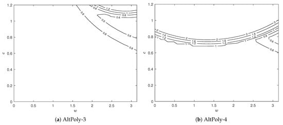
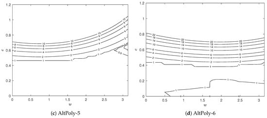
Figure 2.
Contour plots of the principal eigenvalues of the amplification matrices of AltPoly schemes using fourth-order RK time integration for the linear advection equation.
4. Numerical Results
In this part, we solve several types of one-dimensional hyperbolic law to illustrate the performance of the proposed method. We choose the four-stage Runge–Kutta method (20) for the time discretization.
For all numerical experiments, AltPoly-r with the moment number r varying from 3 to 6 are tested on uniform meshes. In addition, we check the accuracy of the proposed method on non-uniform meshes. Non-uniform grids are generated by adding a 40% random perturbation upon the element boundary of the uniform mesh. Specifically, suppose and are separately the cell boundary and cell length for the uniform grid, then the element boundary generated for the non-uniform grid is
where are independently identically distributed random variables, denotes the uniform distribution over , and is the amount of perturbation, which is set as 0.2 in our experiments.
Special attention might be paid to specify the initial values of model variables. This is trivial if the initial profile is analytically given. Otherwise, these unknowns can be specified by implementing high-order interpolations and numerical integration.
Since the temporal accuracy is only fourth-order, we take for AltPoly-r in the accuracy tests.
4.1. Linear Scalar Equation
In this subsection, we test the performance of AltPoly schemes on the following scalar equation [29]:
We first check the accuracy of the proposed method through grid refinement tests. The initial condition is given as with a periodical boundary condition on . The exact solution is . We refine the grid and record numerical errors after one period ().
Two typical norms for errors are adopted here, i.e., and The errors and the convergence rates are presented in Table 1. We can see that the spatial accuracy order is for the AltPoly-r scheme, which matches our theoretical analysis in Section 3. Additionally, the order of accuracy is also maintained well for non-uniform meshes.

Table 1.
Accuracy test for linear hyperbolic law with initial condition at .
Next, we use a complicated initial condition from [30] to evaluate the ability of the proposed method in handling both continuous and discontinuous profiles. This initial condition contains four piece-wise functions:
where the involved functions are
and
with the constants set as , and As for the initial profile, we suggest using the routine used in the discontinuous Galerkin method.
A smaller time step can help reduce the oscillations around discontinuities. We take , and , respectively, for AltPoly-3, AltPoly-4, AltPoly-5, and AltPoly-6.
The computational domain is divided into 200 elements. We first compute this problem without adding artificial viscosity, for which higher-order methods can produce better results in both continuous and discontinuous regions. The results at are illustrated in Figure 3 and Figure 4 separately. Specifically, AltPoly-3 and AltPoly-4 generate significant oscillations around and . These oscillations are reasonable as our method is based on the smoothness assumption and the polynomial does have its limitations on presenting discontinuities. However, it is interesting that spurious oscillations are significantly reduced and the transitions around strong discontinuities are quite sharp for AltPoly-5 and AltPoly-6. After adding a proper amount of artificial viscosity, the proposed method is able to smooth the artificial oscillations for AltPoly method of various orders while not losing high accuracy in the smooth regions.
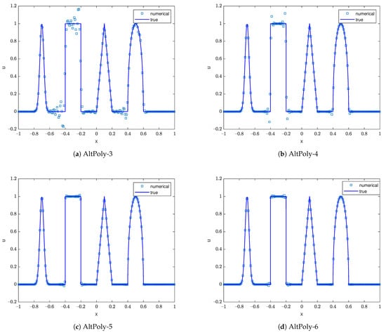
Figure 3.
Numerical results of the advection of a complicated profile at via AltPoly without artificial viscosity using cells.
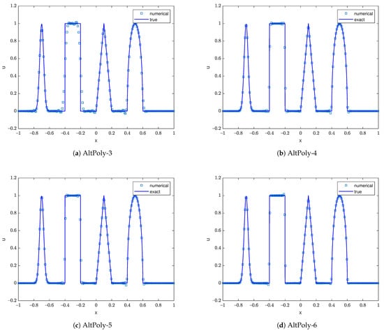
Figure 4.
Numerical results of the advection of a complicated profile at via AltPoly with artificial viscosity using cells.
4.2. Nonlinear Burgers Equation
This subsection considers the 1D inviscid Burgers equation
The initial condition is for with the periodical boundary condition.
Although the initial profile is smooth, shock waves exist when t is large enough since the flux function is nonlinear. To evaluate the order of accuracy, we calculate the numerical solution before the shock wave occurs and compute the errors in respect of grid refinement. Table 2 lists the errors at when the solution is still smooth. The numerical convergence rate results are consistent with our theoretical analysis.
Table 2.
Accuracy test for Burgers equation with at .
The numerical results for the Burgers equation at are shown in Figure 5 when a shock has already emerged. To handle the shock discontinuity, we add a proper amount of artificial viscosity according to Section 2.4. We can see that our schemes suppress the oscillations well around the discontinuity while still maintaining a sharp and accurate profile.
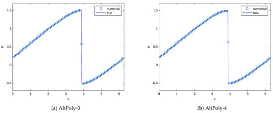
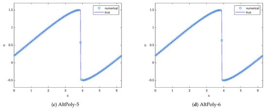
Figure 5.
Numerical results of the Burgers equation at with cells and
4.3. Euler Equations
We then use our scheme to solve the one-dimensional Euler system:
where refers to the density, u the velocity, the momentum, e the total energy, and p the pressure:
with for a perfect dry gas. Just like in the scalar case, we introduce point-valued and cell-averaged moments for each variable. The cell-averaged moments are updated by the flux-form Equation (56). In Step 2 of AltPoly, solution values on auxiliary points are updated using the following non-conservative form equations:
where
Neither characteristic decomposition nor Riemann solver are needed here.
We first check the order of accuracy for this nonlinear system by simulating advection of the density perturbation. The initial conditions are , , and for with the periodic boundary condition. The exact solution is a traveling wave: , and . The error results of the density are listed in Table 3 and a satisfactory convergence rate is obtained.
Table 3.
Accuracy test for the one-dimensional Euler equation with at .
We then consider the classical shock tube problem, which is described by Euler equations with the following Riemann-type initial distribution:
Two initial conditions are tested here. The first one is known as Sod’s problem and the initial condition is defined as
The second one is Lax’s problem, which starts from the following initial condition:
We compute these shock tube problems with 100 cells using the AltPoly schemes equipped with the artificial viscosity. Generally, a certain degree of spurious oscillation still exists but is in a tolerant range. As shown in Figure 6 and Figure 7, all AltPoly schemes can depict shocks sharply using only one or two cells. The higher-order schemes (AltPoly-5 and AltPoly-6) capture the contact discontinuities with only one or two cells, while more cells are needed for the lower-order AltPoly schemes.
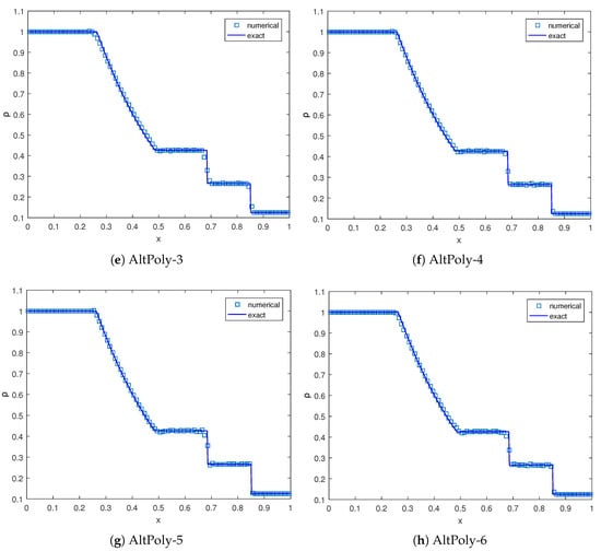
Figure 6.
Numerical results of Sod’s problem at with cells. , , , and , respectively.
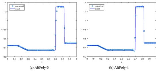
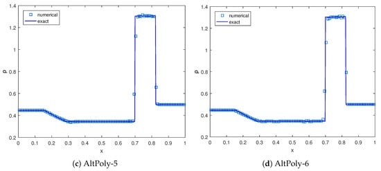
Figure 7.
Numerical results of Lax’s problem at with cells. , , , and , respectively.
To show the accuracy of our smoothness indicator (23), Figure 8 illustrates the cells where the artificial viscosity takes effect on the x-t plane. Generally, the number of cells recognized as discontinuous for lower-order schemes is significantly smaller than that for higher-order schemes. This might be because lower-order schemes have a larger dissipation and the smoothness indicator is less accurate than that of high-order schemes. It is remarkable that the artificial viscosity vanishes in most areas and is in effect only around the shock wave. The contact discontinuity does not trigger the smoothness indicator as it can be smoothed by the artificial viscosity in the first few time steps.
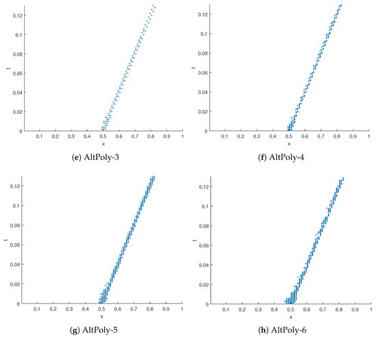
Figure 8.
The cells where artificial viscosity takes effect in Lax’s problem.
5. Conclusions
We have presented a high-order conservative solver termed AltPoly for 1D hyperbolic conservation laws. This method can be categorized as a multi-moment scheme since it adopts both point-values at the middle of the cell and cell-averaged values as the model variables. AltPoly updates the model variables via alternately implementing two polynomial reconstructions. The point-based variables are used to reconstruct a high-order accurate approximation of the solution via Hermite interpolation. The cell-averaged variables updated by the flux-form equations serve as the constraint to guarantee numerical conservation. The solution within a cell is corrected by polynomial reconstruction via solving a constrained least-squares problem. In other words, our method directly reconstructs the solution to maintain the conservation, which is different from existing schemes based on the local flux reconstruction. Fourier analysis shows the accuracy and the admissible range of the CFL number for the linear scalar equation. Further, our scheme can be extended to other kinds of PDEs such as parabolic equations, advection–diffusion equations, etc., which will be our future work.
Author Contributions
S.L., conceptualization, methodology, software, validation, writing—original draft preparation; Q.L., methodology, formal analysis, validation, writing—review and editing; H.L., supervision, methodology, writing—review and editing; J.S., project administration, resources. All authors have read and agreed to the published version of the manuscript.
Funding
This work was supported by National Natural Science Foundation of China No. 41605070.
Institutional Review Board Statement
Not applicable.
Informed Consent Statement
Not applicable.
Data Availability Statement
Not applicable.
Conflicts of Interest
The authors declare no conflict of interest.
Appendix A. Outline of AltPoly-r
Steps 1 and 2 of AltPoly-r are almost the same as those of AltPoly-3 and are hence omitted here. In this part, we focus on introducing the constrained polynomial reconstruction in Step 3 of AltPoly-r for .
Following the notations in Section 2.2.3, the core of Step 3 is reconstructing the polynomial from the following conditions:
where and are obtained in Step 2. Since the hyperbolic conservation law must be obeyed, we rewrite the constraint condition (A2) into the expression of ,
and plug it into (A1) to arrive at
We rewrite it in matrix form:
where
This linear system is overdetermined since it has unknowns and equations. The least-squares solution is
where denotes the generalized inverse or Moore–Penrose inverse [27] of . From we can obtain the updated point-based model variables.
In practice, we find that has a large condition number when and we calculate it via symbolic computation using mathematical software to reduce the error. Throughout this paper, we used the symmetrical solution points for AltPoly-r with the choices of shown in Table A1. Through numerical experiments, we found that smaller can generally induce a more stable numerical scheme, which allows for a larger CFL number. However, when approaches 0, the condition number of tends to infinity, which will cause a loss of accuracy. Based on numerical trials, the choices of are determined as a compromise between stability and accuracy.
Table A1.
Choice of for solution points.
Table A1.
Choice of for solution points.
| r | Solution Points |
|---|---|
| 3 | |
| 4 | |
| 5 | |
| 6 |
Appendix B. Some Technical Results Used in Section 3
Via symbolic computation by Mathematica, we have the following Taylor expansions in decimal form:
where the vectors and are independent with w.
We can see that the magnitudes of all entries in are smaller than 1 when w is small enough. In addition, from (39) we know that
Therefore the principal eigenvalue of is 1 as long as w is small enough.
Now we try to bound and . We first assume that for any , which naturally holds as long as the scheme is stable. Then we have
Hence,
Since the magnitude of is not greater than and , then can be estimated by
As for , the following bound can be deduced based on (A12),
References
- Lele, S.K. Compact finite difference schemes with spectral-like resolution. J. Comput. Phys. 1992, 103, 16–42. [Google Scholar] [CrossRef]
- Mohebbi, A.; Dehghan, M. High order compact solution of the one-space-dimensional linear hyperbolic equation. Numer. Methods Part. Differ. Equ. Int. J. 2008, 24, 1222–1235. [Google Scholar] [CrossRef]
- Yabe, T.; Ishikawa, T.; Wang, P.; Aoki, T.; Kadota, Y.k.; Ikeda, F. A universal solver for hyperbolic equations by cubic-polynomial interpolation II. Two-and three-dimensional solvers. Comput. Phys. Commun. 1991, 66, 233–242. [Google Scholar] [CrossRef]
- Yabe, T.; Xiao, F.; Utsumi, T. The constrained interpolation profile method for multiphase analysis. J. Comput. Phys. 2001, 169, 556–593. [Google Scholar] [CrossRef]
- Aoki, T. Interpolated differential operator (IDO) scheme for solving partial differential equations. Comput. Phys. Commun. 1997, 102, 132–146. [Google Scholar] [CrossRef]
- Imai, Y.; Aoki, T. Stable coupling between vector and scalar variables for the IDO scheme on collocated grids. J. Comput. Phys. 2006, 215, 81–97. [Google Scholar] [CrossRef]
- Goodrich, J.; Hagstrom, T.; Lorenz, J. Hermite methods for hyperbolic initial-boundary value problems. Math. Comput. 2006, 75, 595–630. [Google Scholar] [CrossRef] [Green Version]
- Tanaka, R.; Nakamura, T.; Yabe, T. Constructing exactly conservative scheme in a non-conservative form. Comput. Phys. Commun. 2000, 126, 232–243. [Google Scholar] [CrossRef]
- Yabe, T.; Tanaka, R.; Nakamura, T.; Xiao, F. An exactly conservative semi-Lagrangian scheme (CIP–CSL) in one dimension. Mon. Weather Rev. 2001, 129, 332–344. [Google Scholar] [CrossRef]
- Imai, Y.; Aoki, T.; Takizawa, K. Conservative form of interpolated differential operator scheme for compressible and incompressible fluid dynamics. J. Comput. Phys. 2008, 227, 2263–2285. [Google Scholar] [CrossRef]
- Onodera, N.; Aoki, T.; Kobayashi, H. Large-eddy simulation of turbulent channel flows with conservative IDO scheme. J. Comput. Phys. 2011, 230, 5787–5805. [Google Scholar] [CrossRef]
- Ii, S.; Shimuta, M.; Xiao, F. A 4th-order and single-cell-based advection scheme on unstructured grids using multi-moments. Comput. Phys. Commun. 2005, 173, 17–33. [Google Scholar] [CrossRef]
- Cockburn, B.; Shu, C.W. TVB Runge-Kutta local projection discontinuous Galerkin finite element method for conservation laws. II. General framework. Math. Comput. 1989, 52, 411–435. [Google Scholar]
- Cockburn, B.; Lin, S.Y.; Shu, C.W. TVB Runge-Kutta local projection discontinuous Galerkin finite element method for conservation laws III: One-dimensional systems. J. Comput. Phys. 1989, 84, 90–113. [Google Scholar] [CrossRef] [Green Version]
- Qiu, J.; Shu, C.W. Runge–Kutta discontinuous Galerkin method using WENO limiters. SIAM J. Sci. Comput. 2005, 26, 907–929. [Google Scholar] [CrossRef]
- Wang, Z.J. Spectral (finite) volume method for conservation laws on unstructured grids. basic formulation: Basic formulation. J. Comput. Phys. 2002, 178, 210–251. [Google Scholar] [CrossRef] [Green Version]
- Wang, Z.J.; Zhang, L.; Liu, Y. Spectral (finite) volume method for conservation laws on unstructured grids IV: Extension to two-dimensional systems. J. Comput. Phys. 2004, 194, 716–741. [Google Scholar] [CrossRef]
- Liu, Y.; Vinokur, M.; Wang, Z.J. Spectral difference method for unstructured grids I: Basic formulation. J. Comput. Phys. 2006, 216, 780–801. [Google Scholar] [CrossRef]
- Huynh, H.T. A flux reconstruction approach to high-order schemes including discontinuous Galerkin methods. In Proceedings of the 18th AIAA Computational Fluid Dynamics Conference, Miami, FL, USA, 25–28 June 2007; p. 4079. [Google Scholar]
- Wang, Z.J.; Gao, H. A unifying lifting collocation penalty formulation including the discontinuous Galerkin, spectral volume/difference methods for conservation laws on mixed grids. J. Comput. Phys. 2009, 228, 8161–8186. [Google Scholar] [CrossRef]
- Ii, S.; Xiao, F. High order multi-moment constrained finite volume method. Part I: Basic formulation. J. Comput. Phys. 2009, 228, 3669–3707. [Google Scholar] [CrossRef] [Green Version]
- Xiao, F.; Ii, S.; Chen, C.; Li, X. A note on the general multi-moment constrained flux reconstruction formulation for high order schemes. Appl. Math. Model. 2013, 37, 5092–5108. [Google Scholar] [CrossRef]
- Kirby, R.M.; Karniadakis, G.E. De-aliasing on non-uniform grids: Algorithms and applications. J. Comput. Phys. 2003, 191, 249–264. [Google Scholar] [CrossRef] [Green Version]
- Kanevsky, A.; Carpenter, M.H.; Hesthaven, J.S. Idempotent filtering in spectral and spectral element methods. J. Comput. Phys. 2006, 220, 41–58. [Google Scholar] [CrossRef]
- Zienkiewicz, O.C.; Taylor, R.L.; Zhu, J.Z. The Finite Element Method: Its Basis and Fundamentals; Elsevier: Amsterdam, The Netherlands, 2005. [Google Scholar]
- Staniforth, A.; Côté, J. Semi-Lagrangian integration schemes for atmospheric models—A review. Mon. Weather Rev. 1991, 119, 2206–2223. [Google Scholar] [CrossRef] [Green Version]
- Ben-Israel, A.; Greville, T.N. Generalized Inverses: Theory and Applications; Springer Science & Business Media: Berlin/Heidelberg, Germany, 2003; Volume 15. [Google Scholar]
- Persson, P.O.; Peraire, J. Sub-cell shock capturing for discontinuous Galerkin methods. In Proceedings of the 44th AIAA Aerospace Sciences Meeting and Exhibit, Reno, NV, USA, 9–12 January 2006; p. 112. [Google Scholar]
- Dehghan, M.; Shokri, A. A meshless method for numerical solution of a linear hyperbolic equation with variable coefficients in two space dimensions. Numer. Methods Part. Differ. Equ. Int. J. 2009, 25, 494–506. [Google Scholar] [CrossRef]
- Jiang, G.S.; Shu, C.W. Efficient implementation of weighted ENO schemes. J. Comput. Phys. 1996, 126, 202–228. [Google Scholar] [CrossRef] [Green Version]
Publisher’s Note: MDPI stays neutral with regard to jurisdictional claims in published maps and institutional affiliations. |
© 2021 by the authors. Licensee MDPI, Basel, Switzerland. This article is an open access article distributed under the terms and conditions of the Creative Commons Attribution (CC BY) license (https://creativecommons.org/licenses/by/4.0/).