
Theory and Applications of the Unit Gamma/Gompertz Distribution


Abstract
:1. Introduction
2. Primary Functions
2.1. Cumulative Distribution Function
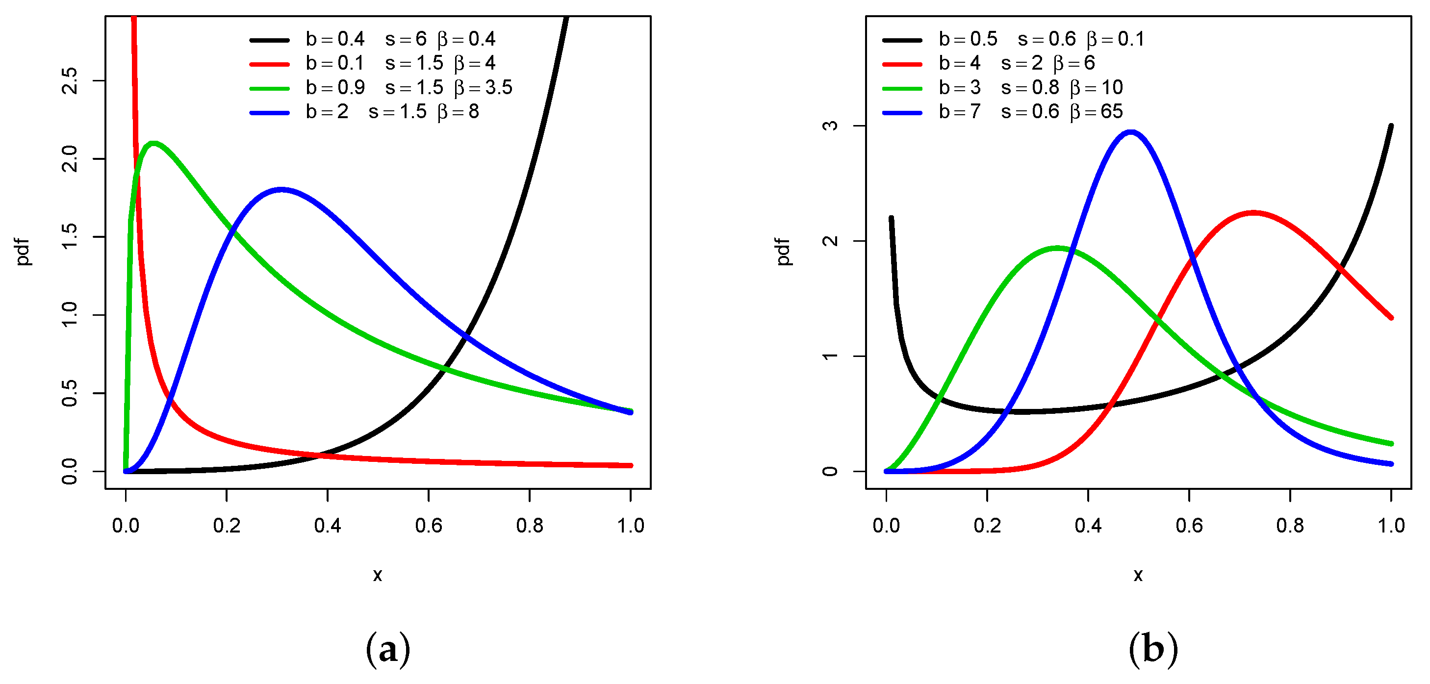
2.2. Probability Density Function
- If or , then is monotonic. In particular:
- –
- If , is increasing.
- –
- If , is decreasing.
- If , then is non-monotonic. In particular:
- –
- If , is “increasing-decreasing”.
- –
- If , is “decreasing-increasing”.
2.3. Survival and Hazard Rate Functions
3. Relevant Properties
3.1. Distributional Inequalities
- decreasing with respect to the parameter b,
- decreasing with respect to the parameter s,
- increasing with respect to the parameter β.
- After several developments, we establish thatThus, the function is decreasing with respect to the parameter b.
- With the same approach, we haveSincewe have , and the function is decreasing with respect to the parameter s.
- Algebraic operations provideAs a result, the function is increasing with respect to the parameter . Proposition 2 is proven. □
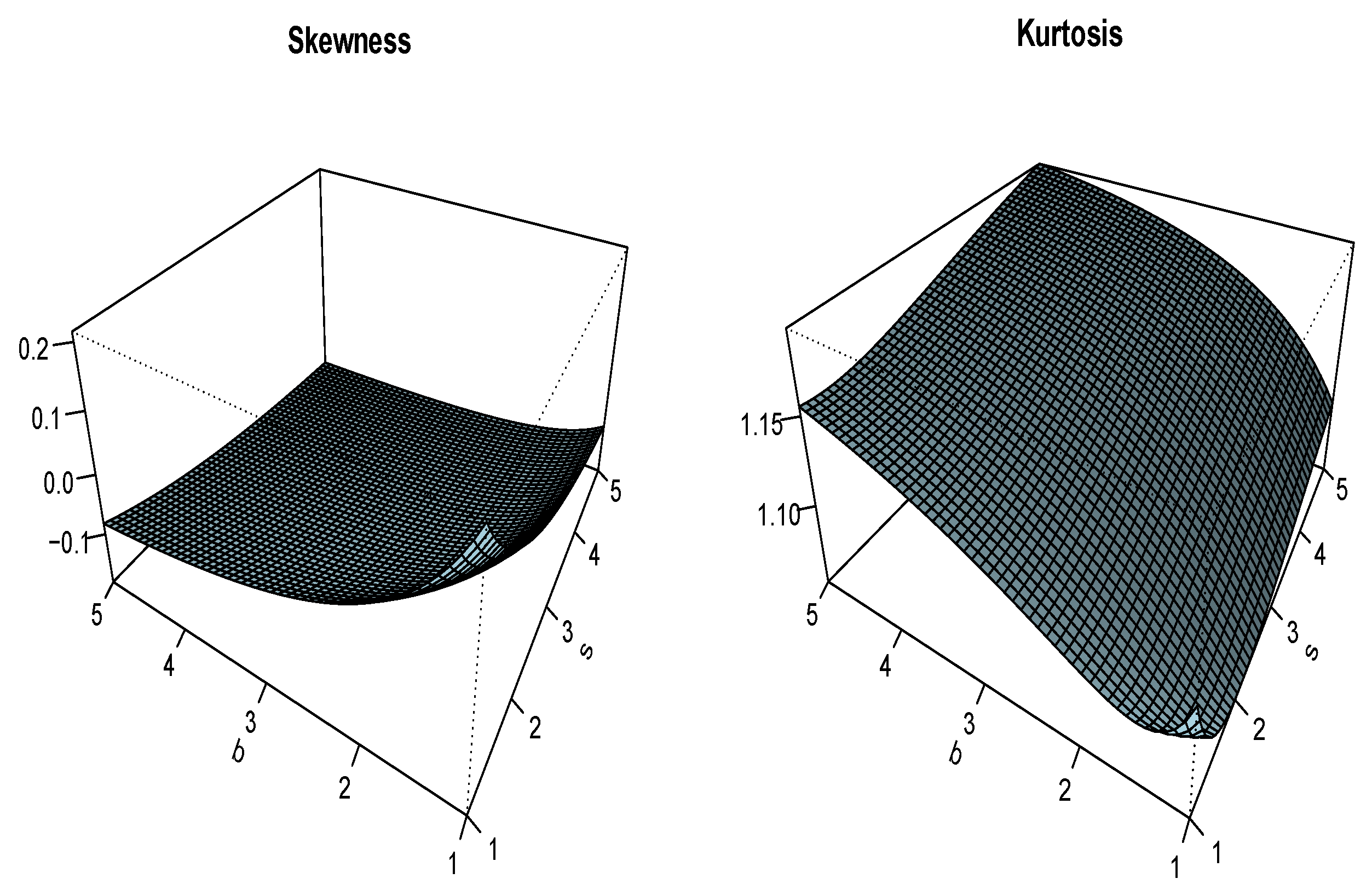
3.2. Moment Properties
3.3. Quantile Properties
3.4. Reliability Coefficient
4. Estimation with Simulation
4.1. Estimation
4.2. Simulation
- We generate 5000 random samples of the form from the UG/G distribution, where, using Equation (6), is calculated by the following formula:where denotes a sample of values generated from the uniform distribution over .
- Different sample sizes are considered as , 200, 300, and 1000.
- Five different configurations for the vector of parameters are chosen as Config1: , Config2: , Config3: , Config4: , and Config5: .
- The average MLEs, mean square errors (MSEs), CI-Ls, CI-Us, and lengths (LENs) of the CIs with two different levels (90% and 95%) for the considered configurations are calculated.
5. Applications
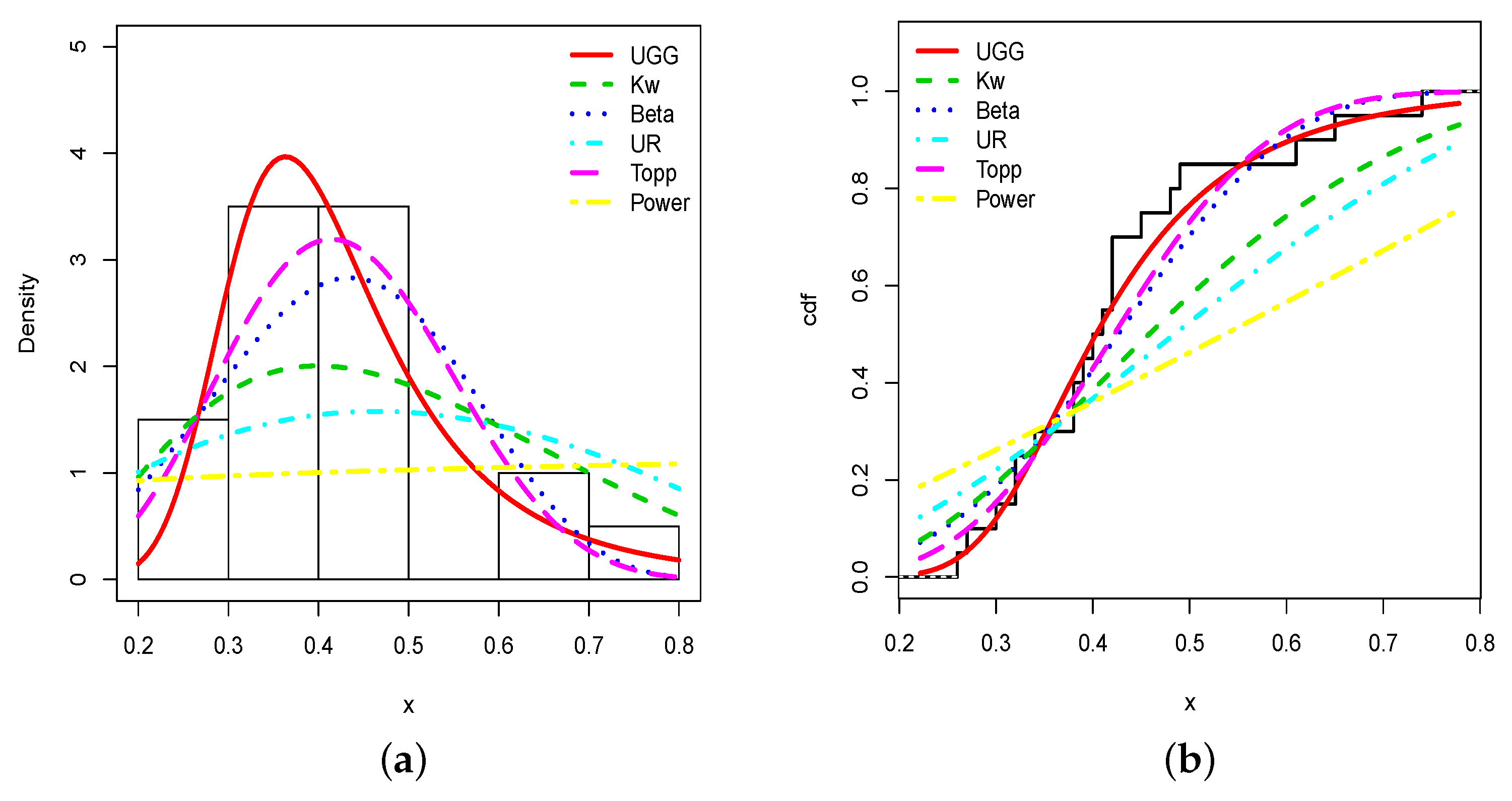
5.1. Application 1
- Kw distribution:for , and for , with .
- Beta distribution:with , for , and for , with .
- UR distribution:for , and for , with .
- Topp distribution:for , and for , with .
- Power distribution:for , and for , with .
- TM distribution:for , and for , with .
5.2. Application 2
5.3. Complementary Analysis
6. Conclusions
Author Contributions
Funding
Institutional Review Board Statement
Informed Consent Statement
Data Availability Statement
Acknowledgments
Conflicts of Interest
Appendix A
References
- Aitchison, J. The statistical analysis of compositional data. J. R. Stat. Soc. Ser. B (Methodol.) 1982, 44, 139–177. [Google Scholar] [CrossRef]
- Consul, P.C.; Jain, G.C. On the log-gamma distribution and its properties. Stat. Pap. 1971, 12, 100–106. [Google Scholar] [CrossRef]
- Gómez-Déniz, E.; Sordo, M.A.; Calderín-Ojeda, E. The log-Lindley distribution as an alternative to the beta regression model with applications in insurance. Insur. Math. Econ. 2014, 54, 49–57. [Google Scholar] [CrossRef]
- Mazucheli, J.; Menezes, A.F.B.; Ghitany, M.E. The unit-Weibull distribution and associated inference. J. Appl. Probab. Stat. 2018, 13, 1–22. [Google Scholar]
- Mazucheli, J.; Menezes, A.F.B.; Fernandes, L.B.; De Oliveira, R.P.; Ghitany, M.E. The unit-Weibull distribution as an alternative to the Kumaraswamy distribution for the modeling of quantiles conditional on covariates. J. Appl. Stat. 2020, 47, 954–974. [Google Scholar] [CrossRef]
- Mazucheli, J.; Menezes, A.F.B.; Dey, S. Unit-Gompertz Distrib. Applications. Statistica 2019, 79, 25–43. [Google Scholar]
- Korkmaz, M.Ç.; Chesneau, C. On the unit Burr-XII distribution with the quantile regression modeling and applications. Comput. Appl. Math. 2021, 40, 29. [Google Scholar] [CrossRef]
- Altun, E. The log-weighted exponential regression model: Alternative to the beta regression model. Commun. Stat.-Theory Methods 2021, 50, 2306–2321. [Google Scholar] [CrossRef]
- Altun, E.; Hamedani, G.G. The log-xgamma distribution with inference and application. J. De La Société Française De Stat. 2018, 159, 40–55. [Google Scholar]
- Bantan, R.A.R.; Chesneau, C.; Jamal, F.; Elgarhy, M.; Tahir, M.H.; Aqib, A.; Zubair, M.; Anam, S. Some new facts about the unit-Rayleigh distribution with applications. Mathematics 2020, 8, 1954. [Google Scholar] [CrossRef]
- Bemmaor, A.C.; Glady, N. Modeling purchasing behavior with sudden “death”: A flexible customer lifetime model. Manag. Sci. 2012, 58, 1012–1021. [Google Scholar] [CrossRef]
- Afshar-Nadjafi, B. An iterated local search algorithm for estimating the parameters of the gamma/Gompertz distribution. Model. Simul. Eng. 2014, 2014, 629693. [Google Scholar] [CrossRef] [Green Version]
- Okagbue, H.I.; Adamu, M.O.; Owoloko, E.A.; Opanuga, A.A. Classes of ordinary differential equations obtained for the probability functions of Gompertz and gamma Gompertz distributions. In Proceedings of the World Congress on Engineering and Computer Science 2017, San Francisco, CA, USA, 25–27 October 2017; pp. 405–411. [Google Scholar]
- AzZwideen, R.; Al-Zou’bi, L.M. The transmuted gamma-Gompertz distribution. Int. J. Res.-Granthaalayah 2020, 8, 236–248. [Google Scholar] [CrossRef]
- Okorie, I.E.; AKpanta, A.C.; Ohakwe, J. Marshall-Olkin extended power function distribution. Eur. J. Stat. Probab. 2017, 5, 16–29. [Google Scholar]
- Shaked, M.; Shanthikumar, J.G. Stochastic Orders; Wiley: New York, NY, USA, 2007. [Google Scholar]
- Gilchrist, W. Statistical Modelling with Quantile Functions; CRC Press: Abingdon, UK, 2000. [Google Scholar]
- Kotz, S.; Lumelskii, Y.; Pensky, M. The Stress-Strength Model and Its Generalizations: Theory and Applications; World Scientific: Singapore, 2003. [Google Scholar]
- Casella, G.; Berger, R.L. Statistical Inference; Brooks/Cole Publishing Company: Bel Air, CA, USA, 1990. [Google Scholar]
- R Core Team. R: A Language and Environment for Statistical Computing; R Foundation for Statistical Computing: Vienna, Austria, 2013; Available online: http://www.R-project.org/ (accessed on 20 February 2021).
- Stock, J.H.; Watson, M.W. Introduction to Econometrics, 2nd ed.; Addison Wesley: Boston, MA, USA, 2007; Available online: https://rdrr.io/cran/AER/man/GrowthSW.html (accessed on 20 June 2020).
- Dumonceaux, R.; Antle, C.E. Discrimination between the Log-Normal and the Weibull distributions. Technometrics 1973, 15, 923–926. [Google Scholar] [CrossRef]
- Aarset, M.V. How to identify bathtub hazard rate. IEEE Trans. Reliab. 1987, 36, 106–108. [Google Scholar] [CrossRef]


| S | K | ||||||
|---|---|---|---|---|---|---|---|
| 0.0848 | 0.0457 | 0.0313 | 0.0238 | 0.0385 | 2.7683 | 10.1353 | |
| 0.0255 | 0.0126 | 0.0083 | 0.0062 | 0.0119 | 5.6826 | 38.0804 | |
| 0.0132 | 0.0064 | 0.0042 | 0.0031 | 0.0062 | 8.0598 | 75.1552 | |
| 0.0387 | 0.0190 | 0.1111 | 0.0798 | 0.0624 | 0.7445 | 2.6686 | |
| 0.3333 | 0.1735 | 0.0126 | 0.0094 | 0.0175 | 4.5246 | 24.7938 | |
| 0.7123 | 0.5451 | 0.4380 | 0.3644 | 0.0376 | -0.5479 | 2.5365 | |
| 0.5786 | 0.3823 | 0.2766 | 0.2132 | 0.0474 | 0.0383 | 2.0981 | |
| 0.7699 | 0.6349 | 0.5446 | 0.4791 | 0.0421 | -1.0558 | 3.3949 | |
| 0.5966 | 0.3824 | 0.2598 | 0.1853 | 0.0265 | 0.0043 | 2.7365 | |
| 0.6370 | 0.4337 | 0.3110 | 0.2327 | 0.0278 | -0.1572 | 2.6743 |
| n | MLE | MSE | 90% | 95% | ||||
|---|---|---|---|---|---|---|---|---|
| CI-L | CI-U | LEN | CI-L | CI-U | LEN | |||
| 100 | 0.7832 | 0.3237 | −0.9990 | 2.5653 | 3.5643 | −1.3402 | 2.9066 | 4.2468 |
| 0.4658 | 0.1469 | −0.6565 | 1.5882 | 2.2448 | −0.8715 | 1.8032 | 2.6746 | |
| 0.5403 | 0.0217 | 0.2304 | 0.7703 | 0.5398 | 0.1787 | 0.8219 | 0.6432 | |
| 200 | 0.7412 | 0.3025 | −0.1981 | 1.6806 | 1.8787 | −0.3780 | 1.8604 | 2.2385 |
| 0.5391 | 0.1328 | −0.2259 | 1.3078 | 1.5337 | −0.3728 | 1.4546 | 1.8274 | |
| 0.5205 | 0.0211 | 0.2944 | 0.7466 | 0.4522 | 0.2511 | 0.7899 | 0.5388 | |
| 300 | 0.5968 | 0.2014 | −0.0601 | 1.2537 | 1.3138 | −0.1859 | 1.3795 | 1.5654 |
| 0.5384 | 0.1249 | −0.0273 | 1.2240 | 1.2513 | −0.1471 | 1.3438 | 1.4909 | |
| 0.4499 | 0.0075 | 0.2783 | 0.6215 | 0.3432 | 0.2455 | 0.6544 | 0.4089 | |
| 1000 | 0.5546 | 0.0816 | 0.2020 | 0.9071 | 0.7051 | 0.1345 | 0.9746 | 0.8401 |
| 0.5346 | 0.0429 | 0.2309 | 0.8383 | 0.6074 | 0.1727 | 0.8964 | 0.7237 | |
| 0.4994 | 0.0019 | 0.3817 | 0.5571 | 0.1754 | 0.3649 | 0.5739 | 0.2090 | |
| n | MLE | MSE | 90% | 95% | ||||
|---|---|---|---|---|---|---|---|---|
| CI-L | CI-U | LEN | CI-L | CI-U | LEN | |||
| 100 | 1.1549 | 1.2964 | −2.3567 | 3.9877 | 6.3444 | −2.9641 | 4.5951 | 7.5592 |
| 0.7710 | 0.3566 | −0.9496 | 2.4915 | 3.4412 | −1.2791 | 2.8210 | 4.1001 | |
| 0.5225 | 0.0436 | 0.1247 | 0.9204 | 0.7957 | 0.0485 | 0.9966 | 0.9481 | |
| 200 | 1.1095 | 0.5145 | −0.4835 | 2.7025 | 3.1860 | −0.7886 | 3.0075 | 3.7961 |
| 0.5361 | 0.1180 | −1.0089 | 2.0811 | 3.0900 | −1.3047 | 2.3770 | 3.6817 | |
| 0.4940 | 0.0277 | 0.2668 | 0.7212 | 0.4544 | 0.2233 | 0.7647 | 0.5414 | |
| 300 | 0.8494 | 0.3305 | −0.1723 | 1.8712 | 2.0435 | −0.3680 | 2.0668 | 2.4348 |
| 0.5151 | 0.0326 | −0.0309 | 1.0612 | 1.0921 | −0.1355 | 1.1657 | 1.3012 | |
| 0.4943 | 0.0100 | 0.3269 | 0.6576 | 0.3306 | 0.2953 | 0.6892 | 0.3940 | |
| 1000 | 0.8046 | 0.2140 | 0.2557 | 1.7452 | 1.4896 | 0.1131 | 1.8879 | 1.7748 |
| 0.4977 | 0.0197 | 0.1769 | 0.7186 | 0.5417 | 0.1250 | 0.7705 | 0.6455 | |
| 0.4958 | 0.0045 | 0.4014 | 0.5862 | 0.1848 | 0.3837 | 0.6039 | 0.2202 | |
| n | MLE | MSE | 90% | 95% | ||||
|---|---|---|---|---|---|---|---|---|
| CI-L | CI-U | LEN | CI-L | CI-U | LEN | |||
| 100 | 1.5224 | 1.5864 | −3.0280 | 6.0727 | 9.1008 | −3.8994 | 6.9441 | 10.8435 |
| 0.7189 | 0.2086 | −2.3250 | 3.7628 | 6.0878 | −2.9079 | 4.3457 | 7.2535 | |
| 0.6220 | 0.1336 | 0.2395 | 1.0045 | 0.7650 | 0.1663 | 1.0778 | 0.9115 | |
| 200 | 1.3579 | 0.3145 | −1.5575 | 4.0732 | 5.6308 | −2.0967 | 4.6124 | 6.7090 |
| 0.5978 | 0.1984 | −0.6051 | 1.8007 | 2.4058 | −0.8354 | 2.0311 | 2.8665 | |
| 0.5621 | 0.0271 | 0.3071 | 0.7772 | 0.4701 | 0.2621 | 0.8222 | 0.5601 | |
| 300 | 1.2796 | 0.2757 | −0.1065 | 2.2656 | 2.3721 | −0.3336 | 2.4927 | 2.8263 |
| 0.5868 | 0.1783 | −0.0473 | 1.4209 | 1.4682 | −0.1879 | 1.5614 | 1.7493 | |
| 0.4577 | 0.0081 | 0.2770 | 0.6184 | 0.3414 | 0.2443 | 0.6511 | 0.4068 | |
| 1000 | 1.2109 | 0.0939 | 0.4768 | 2.1450 | 1.6682 | 0.3171 | 2.3047 | 1.9876 |
| 0.4746 | 0.0091 | 0.2083 | 0.7409 | 0.5327 | 0.1573 | 0.7919 | 0.6347 | |
| 0.4833 | 0.0042 | 0.3975 | 0.5690 | 0.1714 | 0.3811 | 0.5854 | 0.2043 | |
| n | MLE | MSE | 90% | 95% | ||||
|---|---|---|---|---|---|---|---|---|
| CI-L | CI-U | LEN | CI-L | CI-U | LEN | |||
| 100 | 0.8165 | 0.3955 | −1.8587 | 3.4916 | 5.3503 | −2.3709 | 4.0039 | 6.3748 |
| 1.3397 | 0.7860 | −2.2552 | 4.9347 | 7.1899 | −2.9436 | 5.6231 | 8.5667 | |
| 0.6501 | 0.1530 | 0.1890 | 1.1113 | 0.9223 | 0.1007 | 1.1996 | 1.0989 | |
| 200 | 0.5776 | 0.1843 | −1.3949 | 2.5502 | 3.9451 | −1.7726 | 2.9279 | 4.7005 |
| 1.5248 | 0.5228 | −1.3644 | 4.4140 | 5.7784 | −1.9177 | 4.9672 | 6.8849 | |
| 0.6354 | 0.1158 | 0.2678 | 1.0393 | 0.7715 | 0.1939 | 1.1132 | 0.9193 | |
| 300 | 0.4614 | 0.0988 | −0.3973 | 1.3200 | 1.7173 | −0.5617 | 1.4844 | 2.0461 |
| 1.5144 | 0.4258 | −0.5995 | 3.6084 | 4.2079 | −1.0024 | 4.0113 | 5.0137 | |
| 0.5331 | 0.0220 | 0.2356 | 0.8305 | 0.5949 | 0.1787 | 0.8875 | 0.7088 | |
| 1000 | 0.4969 | 0.0553 | −0.0350 | 1.0288 | 1.0637 | −0.1368 | 1.1306 | 1.2674 |
| 1.9444 | 0.4116 | 0.1399 | 2.7490 | 2.6092 | −0.1100 | 2.9988 | 3.1088 | |
| 0.4988 | 0.0064 | 0.3230 | 0.6745 | 0.3515 | 0.2894 | 0.7082 | 0.4189 | |
| n | MLE | MSE | 90% | 95% | ||||
|---|---|---|---|---|---|---|---|---|
| CI-L | CI-U | LEN | CI-L | CI-U | LEN | |||
| 100 | 0.7018 | 0.4537 | −2.8842 | 4.2877 | 7.1718 | −3.5708 | 4.9744 | 8.5452 |
| 1.1850 | 0.9061 | −2.9198 | 5.2898 | 8.2096 | −3.7058 | 6.0758 | 9.7816 | |
| 0.6178 | 0.1673 | 0.0955 | 1.1400 | 1.0445 | −0.0045 | 1.2401 | 1.2446 | |
| 200 | 0.8635 | 0.3419 | −1.3834 | 3.1103 | 4.4937 | −1.8136 | 3.5406 | 5.3542 |
| 1.1541 | 0.7736 | −2.2933 | 4.6016 | 6.8949 | −2.9535 | 5.2617 | 8.2152 | |
| 0.8574 | 0.1217 | 0.4107 | 1.3042 | 0.8935 | 0.3251 | 1.3898 | 1.0646 | |
| 300 | 0.8141 | 0.1459 | −1.2982 | 2.7264 | 4.0246 | −1.6835 | 3.1118 | 4.7953 |
| 0.9337 | 0.0750 | −1.3201 | 3.1875 | 4.5076 | −1.7517 | 3.6191 | 5.3708 | |
| 0.8273 | 0.0384 | 0.5016 | 1.1129 | 0.6113 | 0.4431 | 1.1715 | 0.7284 | |
| 1000 | 0.8061 | 0.0843 | −1.0367 | 2.7688 | 3.8055 | −1.4011 | 3.1332 | 4.5343 |
| 0.8196 | 0.0463 | −0.9275 | 2.5667 | 3.4942 | −1.2621 | 2.9012 | 4.1633 | |
| 0.8184 | 0.0133 | 0.6501 | 1.0066 | 0.3565 | 0.6160 | 1.0408 | 0.4248 | |
| n | Mean | Median | Standard Deviation | Skewness | Kurtosis | Min | Max |
|---|---|---|---|---|---|---|---|
| 61 | 0.5141 | 0.5277 | 0.1935 | 0.0260 | 2.5525 | 0.1405 | 0.9793 |
| Model | Estimates | ||
|---|---|---|---|
| UG/G | 6.8537 | 0.3533 | 15.1067 |
| (2.6613) | (0.1853) | (0.1043) | |
| Kw | 2.3296 | 2.7629 | - |
| (0.3055) | (0.5550) | - | |
| Beta | 2.7943 | 2.6041 | - |
| (0.4880) | (0.4519) | - | |
| UR | 1.2995 | - | - |
| (0.1663) | - | - | |
| Topp | 2.7391 | - | - |
| (0.3507) | - | - | |
| Power | 1.3288 | - | - |
| (0.1701) | - | - | |
| TM | −0.1917 | - | - |
| (0.3313) | - | - |
| Model | AIC | W | A | KS | KS (p-Value) |
|---|---|---|---|---|---|
| UG/G | −24.4739 | 0.0243 | 0.2392 | 0.0507 | 0.9953 |
| Kw | −23.2502 | 0.0526 | 0.4005 | 0.0689 | 0.9142 |
| Beta | −23.9120 | 0.0490 | 0.3864 | 0.0617 | 0.9629 |
| UR | −24.1938 | 0.0769 | 0.6082 | 0.0963 | 0.5892 |
| Topp | −23.9794 | 0.0458 | 0.3740 | 0.0859 | 0.7258 |
| Power | −2.4955 | 0.0495 | 0.3912 | 0.2213 | 0.0041 |
| TM | 1.6683 | 0.0527 | 0.4046 | 0.1792 | 0.0347 |
| n | Mean | Median | Standard Deviation | Skewness | Kurtosis | Min | Max |
|---|---|---|---|---|---|---|---|
| 20 | 0.4225 | 0.4050 | 0.1244 | 1.0734 | 3.6624 | 0.26 | 0.74 |
| Model | Estimates | ||
|---|---|---|---|
| UG/G | 4.4987 | 7.1872 | 239.2606 |
| (1.4263) | (3.4150) | (2.6653) | |
| Kw | 3.3773 | 12.0018 | |
| (0.6041) | (5.4713) | ||
| Beta | 6.8309 | 9.2364 | |
| (2.1179) | (2.8912) | ||
| UR | 1.1366 | ||
| (0.2541) | |||
| Topp | 2.2412 | ||
| (0.5011) | |||
| Power | 1.7804 | ||
| (0.2487) |
| Model | AIC | W | A | KS | KS (p-Value) |
|---|---|---|---|---|---|
| UG/G | −26.4875 | 0.0442 | 0.2610 | 0.1416 | 0.8168 |
| Kw | −21.9465 | 0.1672 | 0.9746 | 0.2175 | 0.3004 |
| Beta | −24.3671 | 0.1267 | 0.7514 | 0.2062 | 0.3625 |
| UR | −20.2352 | 0.0892 | 0.5367 | 0.2892 | 0.0704 |
| Topp | −12.7627 | 0.1194 | 0.7110 | 0.3409 | 0.0191 |
| Power | 1.7804 | 0.1229 | 0.7300 | 0.3977 | 0.0035 |
| n | S | K | |||
|---|---|---|---|---|---|
| Trade share data set | 61 | 0.5147 | 0.1911 | 0.0275 | 2.5943 |
| Flood level data set | 20 | 0.4270 | 0.1391 | 0.9858 | 3.7457 |
Publisher’s Note: MDPI stays neutral with regard to jurisdictional claims in published maps and institutional affiliations. |
© 2021 by the authors. Licensee MDPI, Basel, Switzerland. This article is an open access article distributed under the terms and conditions of the Creative Commons Attribution (CC BY) license (https://creativecommons.org/licenses/by/4.0/).
Share and Cite
Bantan, R.A.R.; Jamal, F.; Chesneau, C.; Elgarhy, M. Theory and Applications of the Unit Gamma/Gompertz Distribution. Mathematics 2021, 9, 1850. https://doi.org/10.3390/math9161850
Bantan RAR, Jamal F, Chesneau C, Elgarhy M. Theory and Applications of the Unit Gamma/Gompertz Distribution. Mathematics. 2021; 9(16):1850. https://doi.org/10.3390/math9161850
Chicago/Turabian StyleBantan, Rashad A. R., Farrukh Jamal, Christophe Chesneau, and Mohammed Elgarhy. 2021. "Theory and Applications of the Unit Gamma/Gompertz Distribution" Mathematics 9, no. 16: 1850. https://doi.org/10.3390/math9161850
APA StyleBantan, R. A. R., Jamal, F., Chesneau, C., & Elgarhy, M. (2021). Theory and Applications of the Unit Gamma/Gompertz Distribution. Mathematics, 9(16), 1850. https://doi.org/10.3390/math9161850