Modelling Functional Shifts in Two-Species Hypercycles

Abstract

Research on hypercycles focuses on cooperative interactions among replicating species, including the emergence of catalytic parasites and catalytic shortcircuits. Further interactions may be expected to arise in cooperative systems. For instance, molecular replicators are subject to mutational processes and ecological species to behavioural shifts due to environmental and ecological changes. Such changes could involve switches from cooperative to antagonistic interactions, in what we call a functional shift. In this article, we investigate a model for a two-member hypercycle model, considering that one species performs a functional shift. First, we introduce the model dynamics without functional shifts to illustrate the dynamics only considering obligate and facultative cooperation. Then, two more cases maintaining cross-catalysis are considered: (i) a model describing the dynamics of ribozymes where a fraction of the population of one replicator degrades the other molecular species while the other fraction still receives catalytic aid; and (ii) a system in which a given fraction of the population predates on the cooperating species while the rest of the population still receives aid. We have characterised the key bifurcation parameters determining extinction, survival, and coexistence of species. We show that predation, regardless of the fraction that benefits from it, does not significantly change dynamics with respect to the degradative case (i), thus conserving dynamics and bifurcations. Their biological significance is interpreted, and their potential implications for the dynamics of early replicators and ecological species are outlined.

1. Introduction

Hypercycles are catalytic networks of self-replicating species able to catalyse the replication of another single species as they all form a closed loop (see Figure 1a,b) [1,2]. Originally, the hypercycle was suggested to allow for the cooperative selection of competing replicators in the origins of life, ensuring the stability of broad contents of information, contrarily to non-catalytically joint replicators, i.e., quasispecies [3,4]. Hypercycles have been suggested as a possible molecular network of prebiotic replicators involving a crucial step from the transition from inanimate to living chemistry [3,4] due to their potential capacity of maintaining larger stable genetic contents as compared to quasispecies populations under large mutations [1,3]. The interest in hypercycles goes beyond the origin of life problem, being a canonical model to investigate different dynamical systems, including cooperation. The generality of the hypercycle replicator equations has allowed using this model to explore virus replication dynamics [5,6,7,8], neural networks [9,10], the immune system [11], or the emergence of language [12]. Moreover, several hypercycle-like systems have been implemented experimentally. These include coiled-coil peptides [13], yeast cell populations [14], and engineered bacteria growing with catalytic parasites [15].

It has been argued that hypercycle units may need two minimal conditions to be evolutionary stable [4,16], namely, catalytic activity and capacity to store information. Good candidates fulfilling these two conditions are catalytic RNA molecules (ribozymes). RNAs with stem and loop structures, similar to transference RNAs [17], are known to be resistant to hydrolysis [18] and also have replicability potential [19,20]. Ribozymes are short RNA molecules with catalytic activity similar to protein enzymes [21,22] and have been considered as potential candidates for forming the first autonomous, self-replicating molecular systems involved in the origins of life [4,16,19,23,24,25,26]. Different activities have been described for natural and in vitro (e.g., peptide-bond formation [27]) evolved ribozymes. Certain introns can catalyse their own excision (self-cleavage) from single-stranded RNA (ssRNA) [20] and ligase reactions by RNA catalysts can occur even with short RNA sequences [28]. Moreover, the same RNA sequences can catalyse trans-esterification reactions for the elongation of one monomer [20], ligation of two independent ssRNAs [29,30], and cleavage of RNA into smaller sequences [20,22,31,32] (see also [26,33] for reviews). Recent experiments have revealed that the combination of RNAs with cold-adaptative mutations enabled catalysing the synthesis of an RNA sequence longer than itself (adding about 200 nucleotides) [34]. Other experiments have shown the spontaneous formation of catalytic cycles and networks from mixtures of RNA fragments able to self-assemble into self-replicating ribozymes [35], providing evidence for selective advantage of cooperative systems composed of ribozymes.

Hypercycle equations have also been suggested as a suitable modelling framework to investigate the dynamics of cooperation in complex ecosystems [36]. More recently, the hypercycle theory and the spatio-temporal dynamics of cooperative ecological interactions have been reviewed in the framework of landscape ecology [37]. Cooperation arises in a multitude of ecological systems [38,39,40,41,42]. These include alarm calls, coalition formation, predator inspection, cooperative breeding, protection against attacks by predators or conspecifics, or cooperative hunting, among others. Examples of intra-specific cooperation (individuals of the same species cooperate) are found, for instance, in females of the vampire species Desmodus rotundus [43,44,45], which perform cooperative breeding (i.e., reciprocal altruism) by sharing blood between themselves. Cooperative hunting, in which the individuals of a given species cooperate to catch the prey, has been described in lions (Panthera leo) [46], brown hyenas (Hyaena brunnea) [47], wild chimpanzees (Pan troglodites) [48], or the fish species Caranx ignobilis [49]. Invertebrate species, such as arthropods, can also hunt cooperatively: Golden-web spiders (Nephila clavipes) [50], the Stegodyphid spider (Stegodyphus mimosarum) [51], or the heteroptera Microvelia douglasi atrolineata [52]. Examples of inter-specific cooperation (cooperation between individuals of different species) have been described in the deep-sea tube worm Lamellibranchia luymesi and microbial symbionts [40], as well as in arbuscular-mycorrhizal fungi, which form an obligate symbiosis with more than $80\%$ of plant species in all terrestrial habitats [42].

Up to now, most of the research on hypercycles has focused on the dynamics arising from the processes of cooperation between replicators, and some works have also included competition for resources (e.g., available mononucleotides or available space) [3,53] and mutation processes [54,55,56]. In this sense, different architectural changes in hypercycles jeopardising their stability and persistence have been thoroughly investigated to date, mainly considering the so-called catalytic parasites [15,57,58,59,60] and, to a lesser extent, catalytic short-circuits [61,62]. Both catalytic parasites and short-circuits involve modifications in the cyclic catalytic patterns. The former involves the emergence (e.g., via mutation) of a replicator that receives catalysis but does not reciprocate the catalytic aid. The latter involves an internal catalytic connection generating a smaller catalytic cycle within the full system.

Some authors have recently been interested in possible shifts in cooperation among species and have used the hypercycle equations to evaluate the dynamics arising from such shifts [63]. For instance, molecular replicators are subject to mutational processes and ecological species to behavioural shifts due to environmental or ecological changes, and one might expect such species to switch from cooperative to antagonistic interactions in what we call a functional shift. The dynamics arising due to functional shifts in hypercycles are still unexplored. The impact of a shift from catalytic cooperation to directed degradation has recently been studied in small discrete-time hypercycles [63]. For this particular case, it was assumed that one of the hypercycle replicators (ribozyme) became a degrading species instead of being cooperative. To the extent of our knowledge, no works have investigated how these shifts may affect the stability of small hypercycles in time-continuous systems.

Examples of functional shifts between cooperating species are found in different ecosystems. For instance, large fish and mammal pelagic predators (tuna, sharks, dolphins) likely cooperate to locate and handle small pelagic shoals [64], and the predation of sharks on dolphins and tuna has been recorded [65,66]. Seabirds form inter-specific flocks that cooperate to locate food at sea, and the predation that occurs at land while breeding in colonies. Body size drives the predatory matrix, which increases its values when environmental conditions worsen [67,68]. Waterbirds form inter-specific mixed colonies to protect against predators (they can contain several different species of waders, terns, and gulls), but some species may predate opportunistically (especially on eggs and chicks) on heterospecifics or may exert kleptoparasitism for food, especially when the environment is harsher [69,70,71,72,73,74,75]. Although this may be anecdotal, and the cooperation may be subtle, marine mammals may “cooperate” to locate and capture prey, and at the same time, larger species may exert some predation, e.g., killer whales on elephant seals [76].

In this article, we analyse two-species (labeled as $S_1$ and $S_2$) hypercycles considering, together with cooperation, directed degradation and predation (see Figure 1). The paper is organised as follows. In Section 2, we introduce the general model that considers crossed cooperation, competition, and decay of the species and includes the interactions due to the functional shifts. Section 3 contains the results of four different systems that can be studied from the general model by removing some of the interactions. This allows a better comprehension of the dynamics only considering cooperation (plus competition and decay) between species and the dynamical changes arising from directed degradation or predation. First, an obligate two-member hypercycle (Figure 1a), which has been thoroughly investigated in Ref. [53] (see also [77]), is briefly commented. The same system including autonomous self-replication for the two species (see Figure 1b) is explored. Then we explore a hypercycle with a functional shift in a given fraction of $S_2$ population, which is able to degrade $S_1$ while still providing catalytic aid to the first species (Figure 1c). This system is inspired in two populations of ribozymes in which some molecules of one of the species (the rest still receive catalysis) acquires the capacity to degrade the other one, still maintaining the catalytic aid. Finally, we explore a similar system in an ecological context considering that a given fraction of $S_2$ population predates on $S_1$ (the other fraction receiving aid from $S_1$) while maintaining the crossed cooperation. Section 4 is devoted to some conclusions.

2. General Mathematical Model

Let us consider a two-member hypercycle with species $S_1$ and $S_2$, and let $x_1$ and $x_2$ represent their respective concentrations (population numbers). The mathematical model we investigate adds further interactions to a standard two-member hypercycle [53] considering processes of directed degradation or predation between the two species while keeping some degree of cooperation between the hypercycle members. This model is given by the following dynamical system:

$$\left\{\begin{array}{c}{\dot{x}}_1=({\alpha }_1{x}_1+k{x}_1{x}_2)\left(1-\frac{x_1+x_2}{c_0}\right)-\epsilon x_1-(1-\beta ){\epsilon }_{12}{x}_1{x}_2,\hfill \\ {\dot{x}}_2=({\alpha }_2{x}_2+\beta {\eta }_{k}k{x}_1{x}_2)\left(1-\frac{x_1+x_2}{c_0}\right)-{\eta }_{\epsilon }\epsilon x_2+\gamma (1-\beta ){\epsilon }_{12}{x}_1{x}_2,\hfill \end{array}\right.$$

(1)

where all parameters except ${\eta }_k$ and ${\eta }_{\epsilon }$ are assumed to be bound in $I=[0,1]$ (see below), and ${\eta }_k,{\eta }_{\epsilon }\ge 0$. That is, parameters have non-negativity constraints: ${\alpha }_i,k,\epsilon ,\beta ,{\epsilon }_{ij},{\eta }_{k,\epsilon },\gamma \ge 0$, and $c_0>0$, with $i,j=1,2$ and $i\ne j$. Each of the model parameters corresponds to the following biological processes (see also Figure 1):

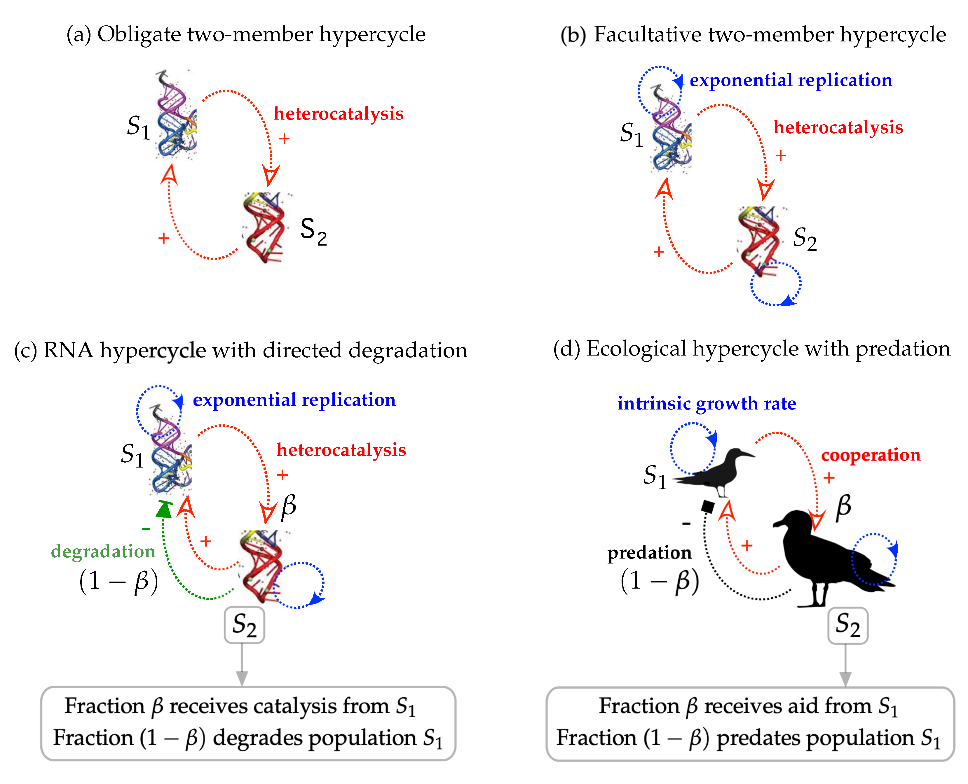
• ${\alpha }_i$: autonomous self-replication rate (Malthusian growth) of species $i=1,2$. ${\alpha }_i\ne 0$ implies that species can replicate themselves without the catalytic aid of the other replicator.
• k: the cross-catalytic replication parameter between $S_1$ and $S_2$. In the case of $S_2$, the term ${\eta }_k$ allows considering a non-symmetric case in which both species are kinetically different. The case ${\eta }_k=1$ involves symmetric catalytic replication.
• $c_0$: known as the carrying capacity, which limits the population of replicators due to finite resources or (implicit) space. Due to the large number of parameters, we will set $c_0=1$.
• $\epsilon$: density-independent spontaneous degradation or death of the species. Analogously to the characteristics of ${\eta }_k$, ${\eta }_{\epsilon }\ne 1$ allows considering a non-symmetric decay scenario for $S_1$ and $S_2$.
• ${\epsilon }_{12}$: the density-dependent degradation rate due to the cleavage (or predation, see below) of species $S_1$ by $S_2$. We notice that the degradative and predatory dynamics are exclusive. That is, we do not consider a case with directed degradation and predation taking place at the same time (these two different cases will be considered with $\gamma =0$ or $\gamma \ne 0$, respectively).
• $\beta$: the fraction of the $S_2$ population still receiving cooperation from $S_1$ replication. The term $1-\beta$ corresponds to the rest of the $S_2$ population that exerts the degradation or the predation of species $S_1$.
• $\gamma$: the energetic efficiency coefficient from predation. It can be understood as the amount of energy species $S_2$ can gain from predating $S_1$ and investing it for reproduction (due to energetic constraints $\gamma <1$). As mentioned, the investigation of the degradative model will be performed by setting $\gamma =0$, while the predatory system will consider $0<\gamma <1$.

As previously mentioned, we focus on parameter values restricted to the interval $I=[0,1]$, except for ${\eta }_k,{\eta }_{\epsilon }$ since we are interested in asymmetric cases. Since the qualitative dynamics mainly depends upon the relative relations between replication/growth and decay/predation parameters, with such an interval we expect to gather all possible dynamics. As mentioned, parameters $\beta$ and $\gamma$ are naturally found within this interval in order to be biologically meaningful. Moreover, the carrying capacity has been set to 1 for simplicity. The choice of a different value for $c_0$ does not change dynamics qualitatively.

It is clear that for the system to hold biological meaning, the phase space is bounded only to the first quadrant of ${\mathbb{R}}^2$. In general terms, the system Equation (1) is able to model the directed degradation of $S_1$ by $S_2$ for values of $0\le \beta <1$ and $\gamma =0$ that becomes fully predatory when $\gamma >0$. The term $1-(x_1+x_2)/c_0$ in Equation (1) is a logistic-like function that introduces competition between the two hypercycle species, also bounding the dynamics.

To provide a general modeling framework and investigate the interplay between cooperation (plus competition and decay) and the functional shifts, i.e., directed degradation or predation, we have kept the cross-catalytic terms. A simpler system considering that species $S_2$ receives aid from $S_1$ and a given fraction $(1-\beta )$, with $0\le \beta <1$, of the $S_2$ population only exerts directed degradation (or predation) on $S_1$ and the rest of the population catalyses $S_1$ can be also investigated by changing $k{x}_1{x}_2$ to $\beta k{x}_1{x}_2$ in ${\dot{x}}_1$; and $\beta {\eta }_{k}k{x}_1{x}_2$ to $\mu {\eta }_k{x}_1{x}_2$ in ${\dot{x}}_2$, $\mu$ being the rate of replication due to the catalysis performed by $S_1$ on $S_2$.

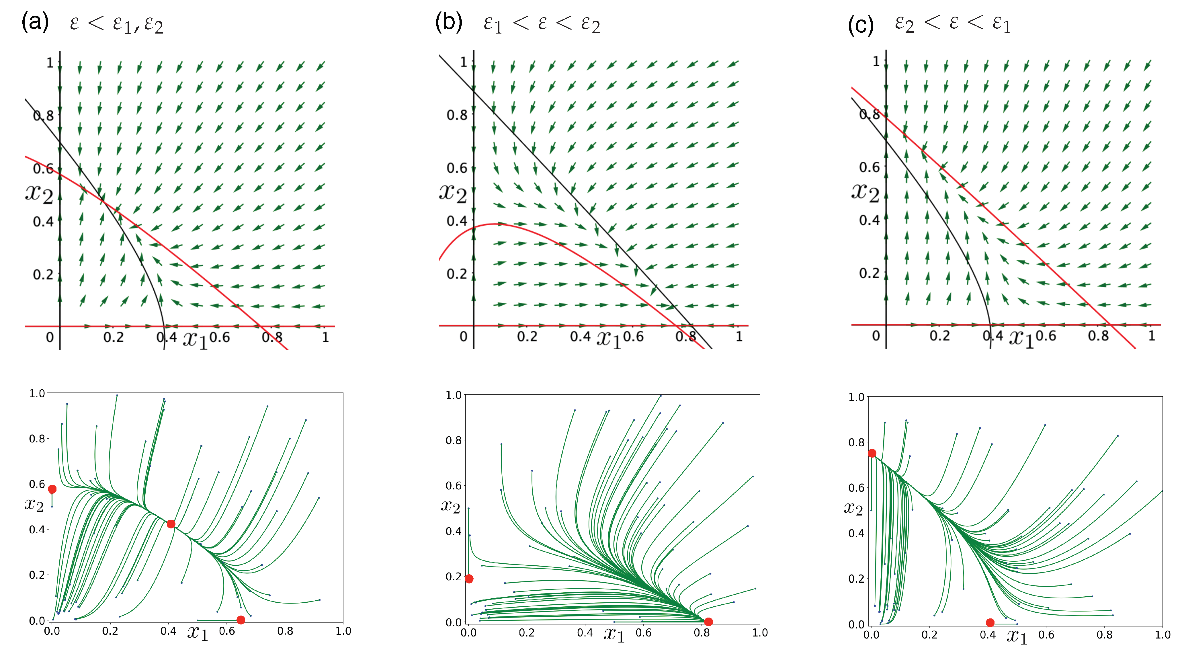
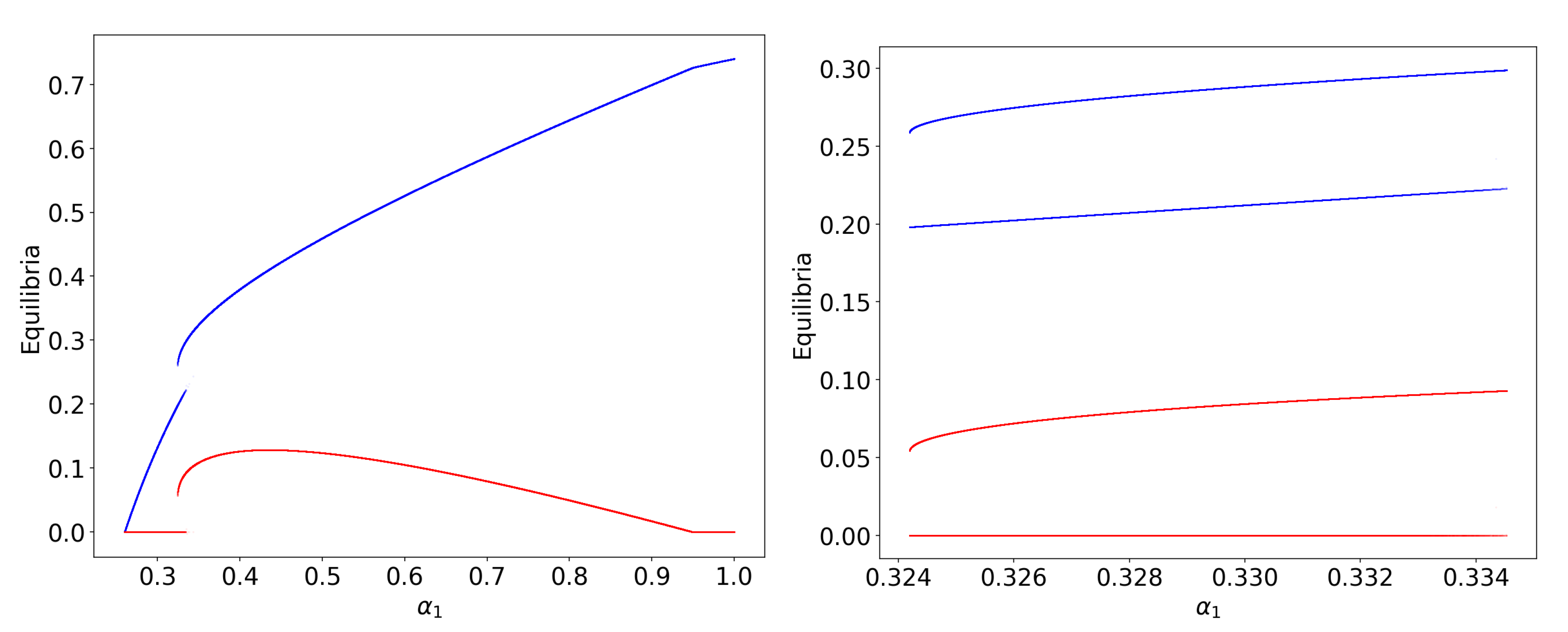
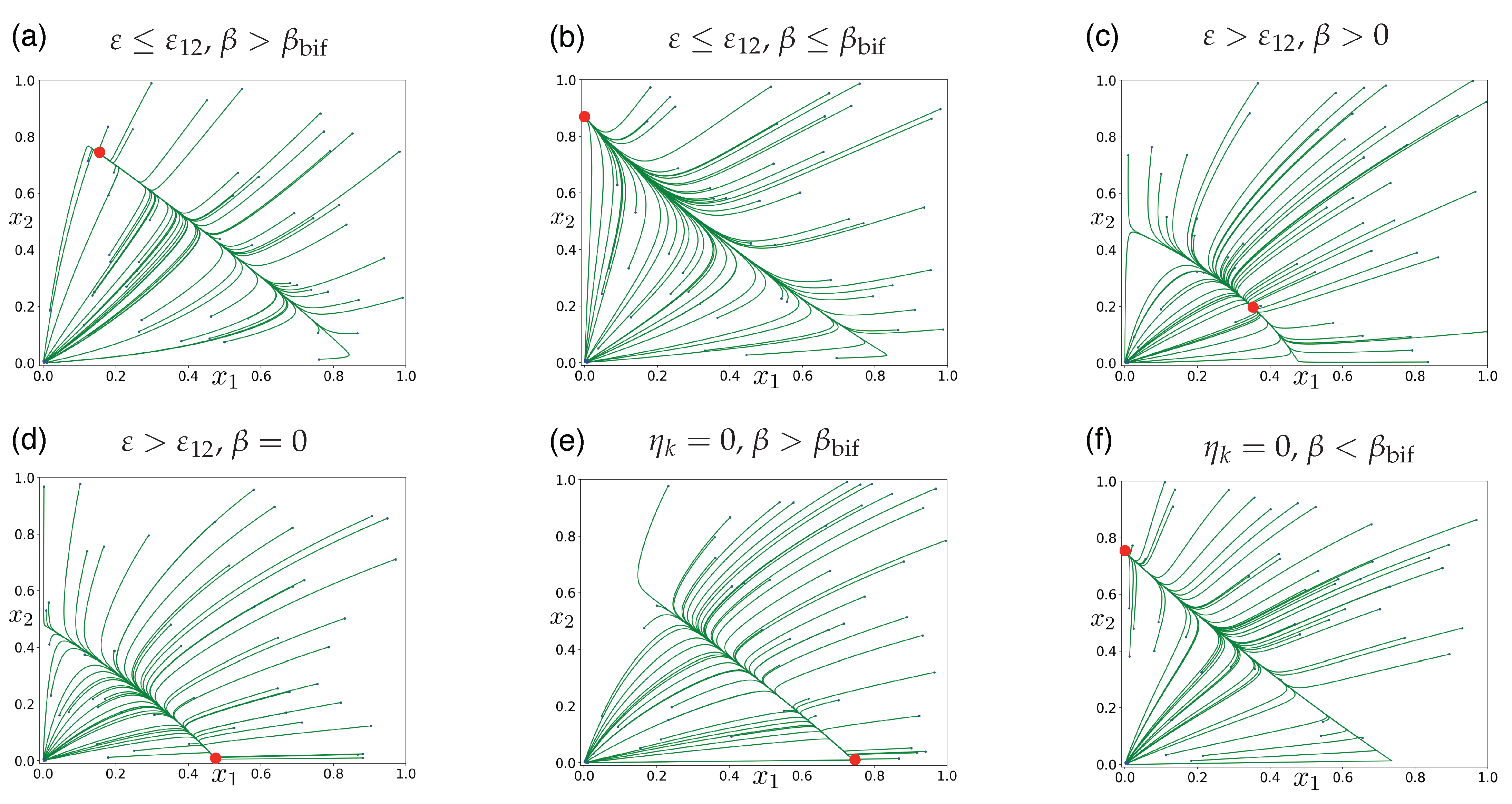
3. Results and Discussion

In this Section, we will investigate the dynamics of Equation (1) considering four different systems. Section 3.1 summarises the results for the obligate two-member hypercycle in which the two species can only replicate catalytically (Figure 1a, see [53,77] for a detailed investigation of this system). Section 3.2 provides further results on this system, including the exponential (non-catalytic) replication of each species. In Section 3.3, we investigate the model considering directed degradation, while Section 3.4 provides further results on the model with predation.

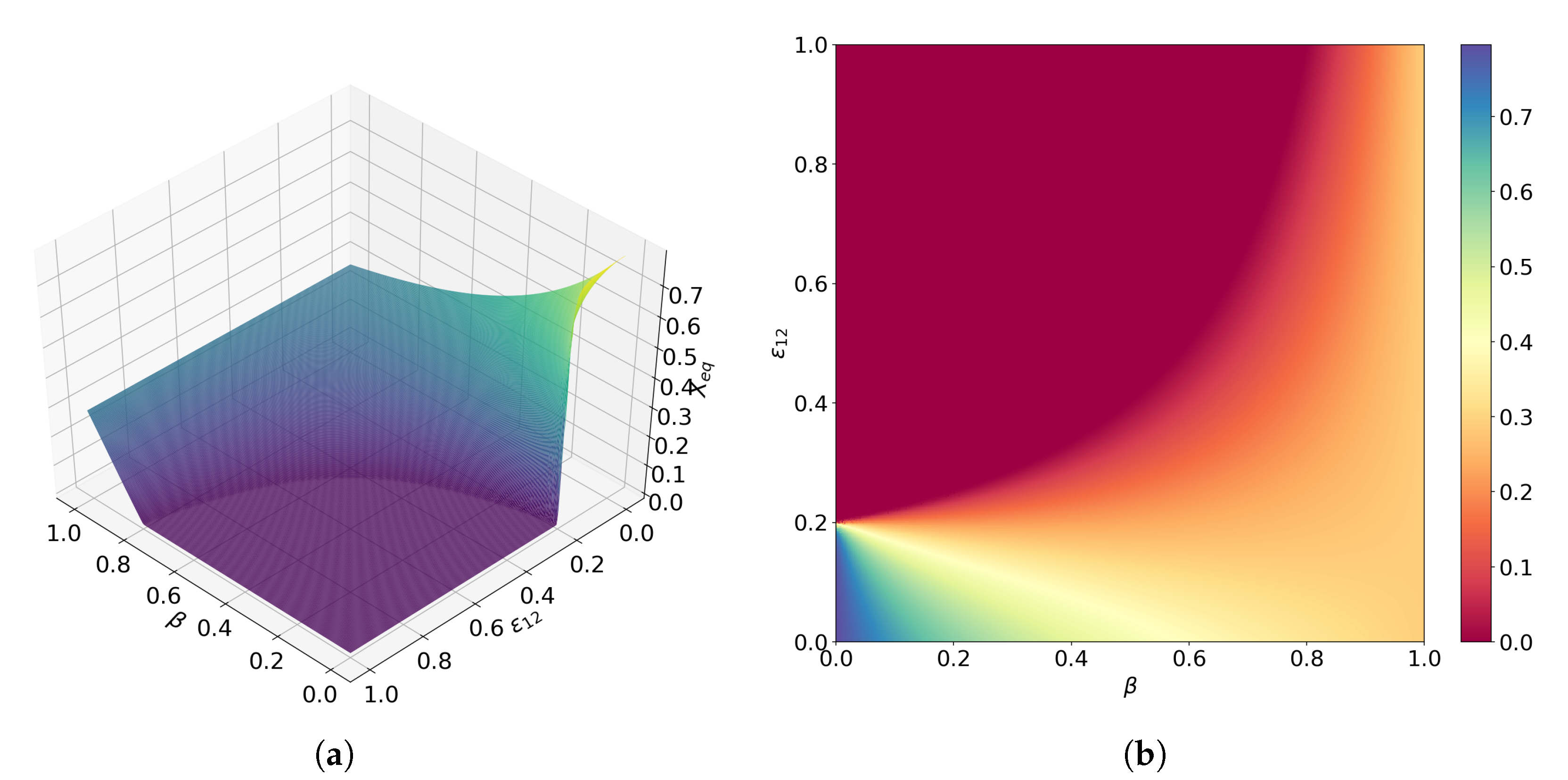
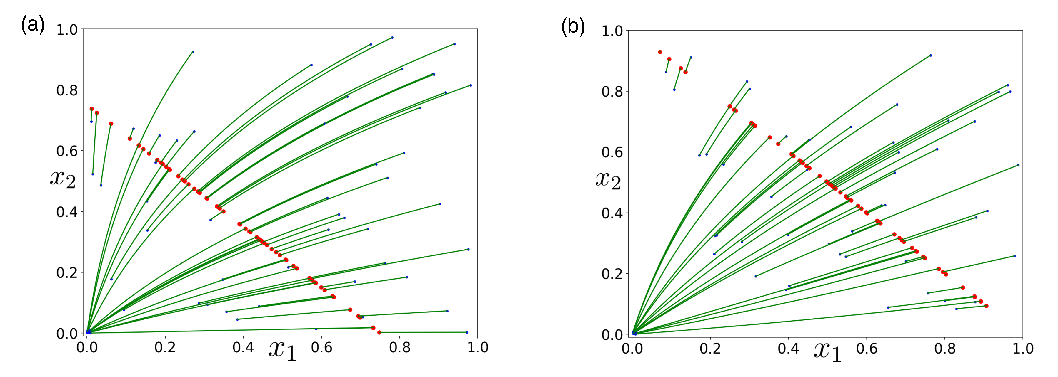
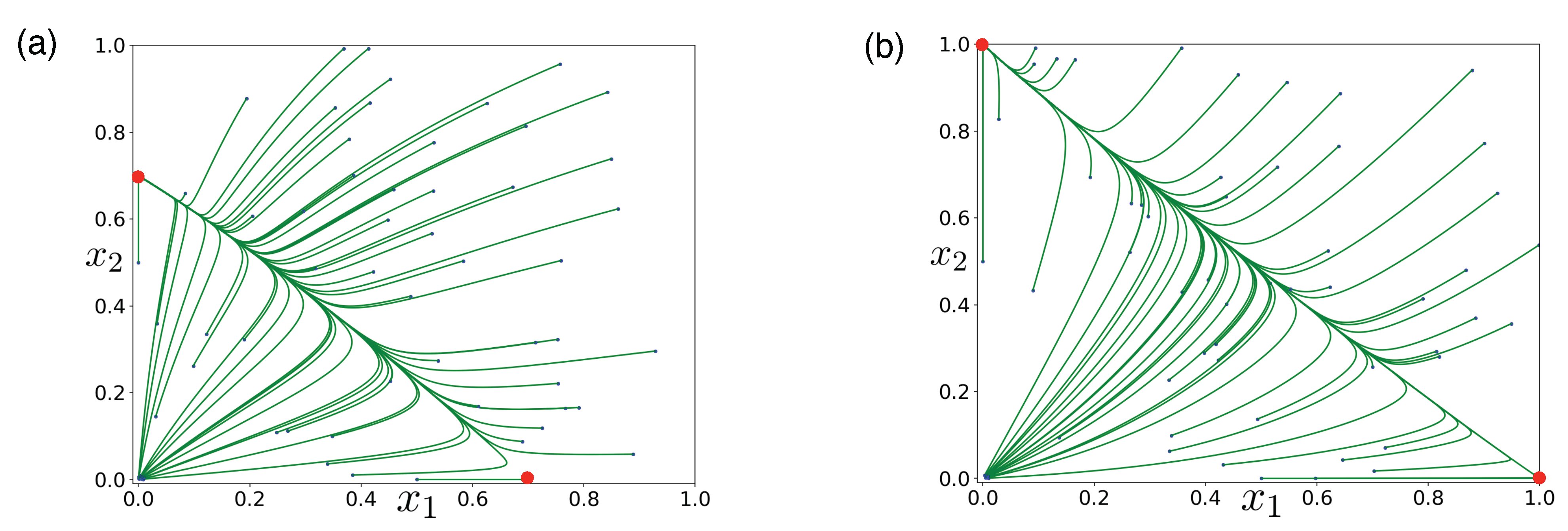
3.1. Obligate Two-Member Hypercycle

Before analysing the models of interest given by directed degradation and predation, it is interesting to start the analysis at a much simpler level. Here, we briefly summarise the dynamics of an obligate two-member hypercycle (Figure 1a). This system, which considers that a species can only replicate due to catalytic (cooperative) processes, can be obtained from Equation (1), setting ${\alpha }_1={\alpha }_2=\gamma =0$ and $\beta =1$. This model is given by

$$\left\{\begin{array}{c}{\dot{x}}_1={\Phi }_1(x_1,x_2)=k{x}_1{x}_2(1-x_1-x_2)-\epsilon x_1,\hfill \\ {\dot{x}}_2={\Phi }_2(x_1,x_2)={\eta }_{k}k{x}_1{x}_2(1-x_1-x_2)-{\eta }_{\epsilon }\epsilon x_2.\hfill \end{array}\right.$$

(2)

This dynamical system was thoroughly investigated in Ref. [53] (see also [77]). The system has three fixed points: the origin $(0,0)$ and the pair $(({\eta }_{\epsilon }/{\eta }_k){\Gamma }_{\pm },{\Gamma }_{\pm })$, where

$${\Gamma }_{\pm }=\frac{1}{2\xi }\left(1\pm \sqrt{1-\frac{4\epsilon \xi }{k}}\right),$$

(3)

and $\xi :=1+{\eta }_{\epsilon }/{\eta }_k$. Note, however, that the expression ${\Gamma }_{\pm }$ is well defined only for $\epsilon \le k/4\xi =:{\epsilon }_c$. Otherwise, ${\Gamma }_{\pm }\in \mathbb{C}$. The origin is a locally asymptotically stable equilibrium, while ${\Gamma }_{-}$ is a saddle point and ${\Gamma }_{+}$ can be either a stable node [53] or a weak stable focus (see Appendix A). The pair ${\Gamma }_{\pm }$ suffers a saddle-node bifurcation at the critical value ${\epsilon }_c$. Above this threshold, the origin becomes globally asymptotically stable (see Ref. [53] for further details and the study of this system using spatially-explicit models).

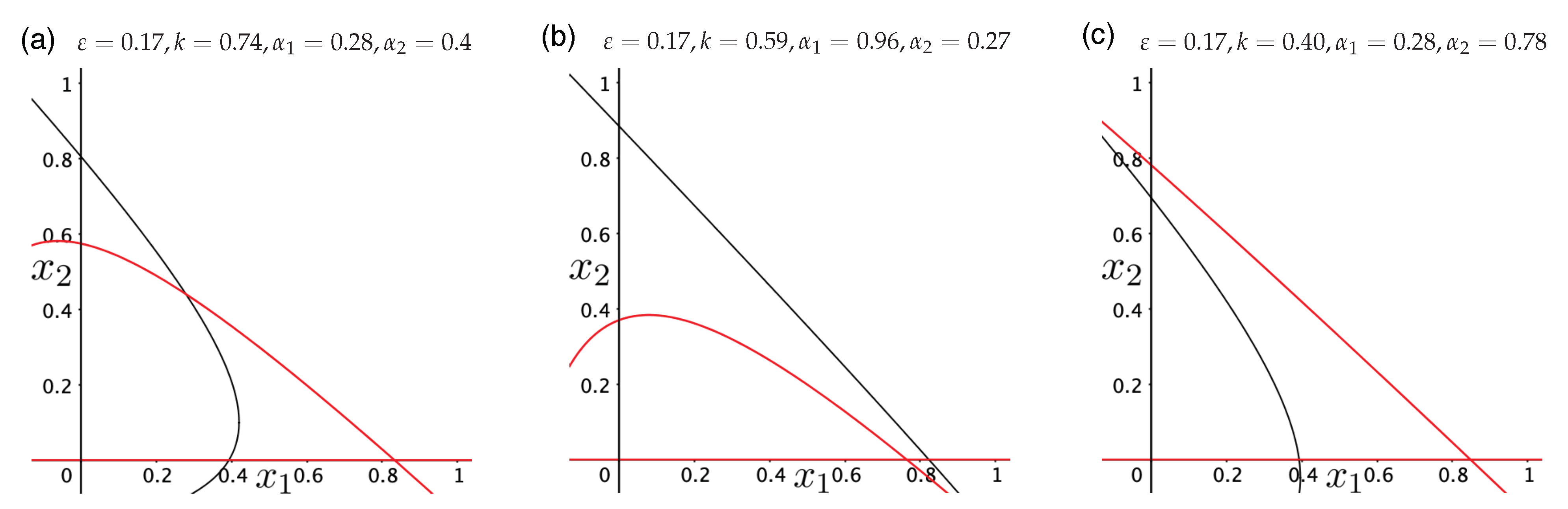
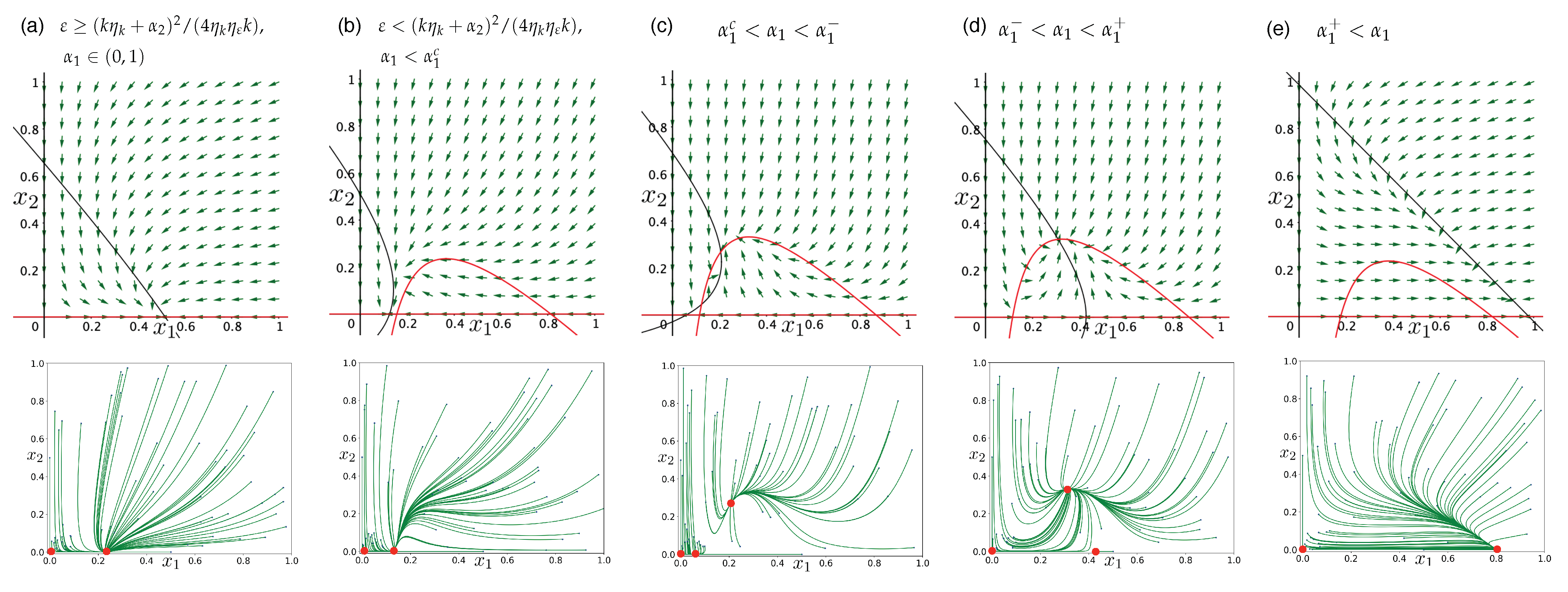
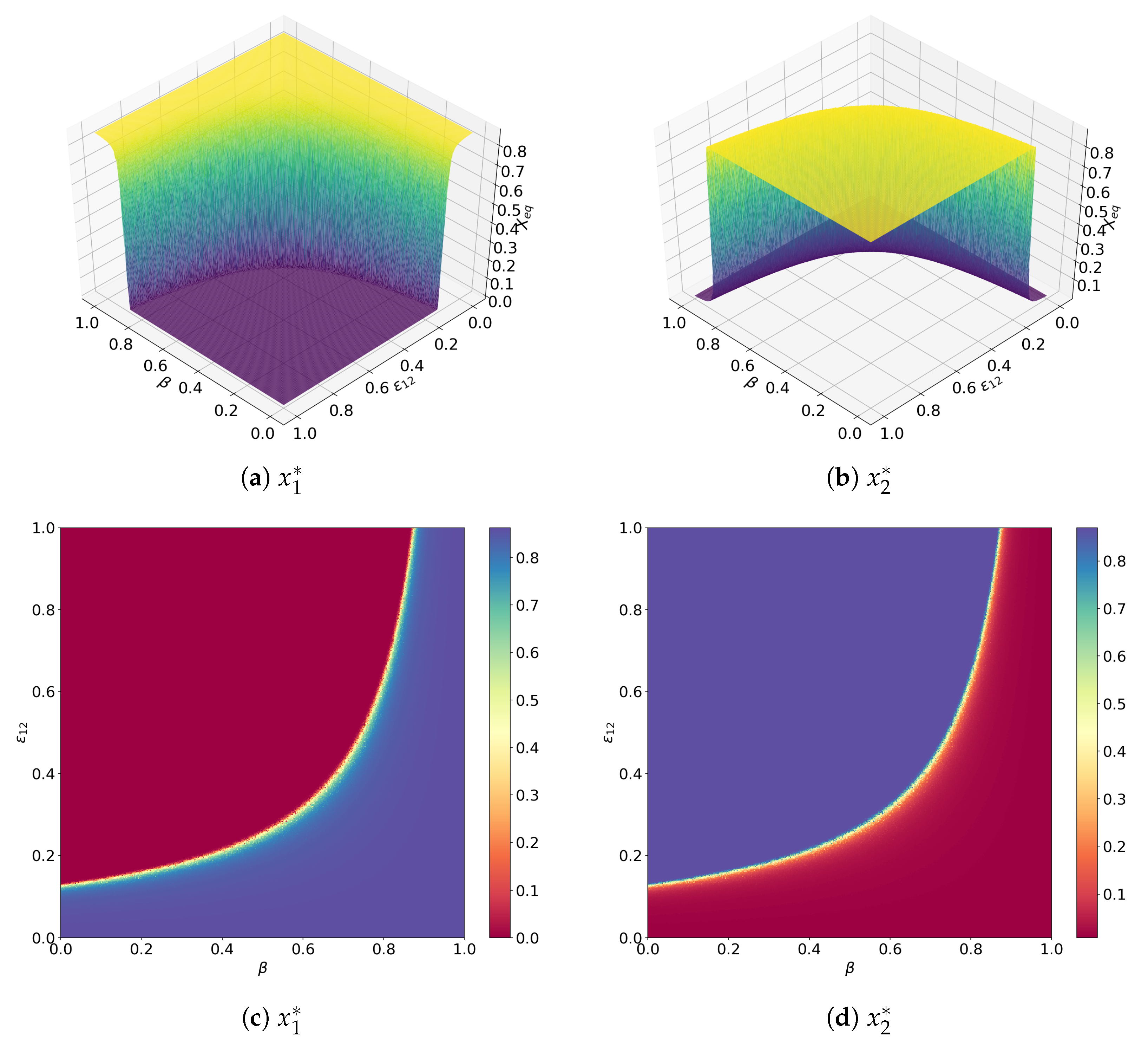
3.2. Facultative Two-Member Hypercycle

The obligate two-member hypercycle is a simple case in which species depend explicitly on the presence of the other to survive. For $S_1$ to replicate, $S_2$ must be present in the system, and vice versa [53]. We shall extend the previous model to a system that considers both exponential replication and cross-catalysis, i.e., facultative hypercycle, proposing a setting that has not been analysed in detail so far (see Refs. [78,79,80] for two-species facultative hypercycles with mutation and error tail). The coupled system of ODEs now involves a parameter of autonomous replication (Malthusian growth), which can be introduced in (1) setting ${\alpha }_{1,2}>0$, while maintaining with $\beta =1$ and $\gamma =0$. We thus consider:

$$\left\{\begin{array}{c}{\dot{x}}_1={\Phi }_1(x_1,x_2)=({\alpha }_1{x}_1+k{x}_1{x}_2)(1-x_1-x_2)-\epsilon x_1,\hfill \\ {\dot{x}}_2={\Phi }_2(x_1,x_2)=({\alpha }_2{x}_2+{\eta }_{k}k{x}_1{x}_2)(1-x_1-x_2)-{\eta }_{\epsilon }\epsilon x_2.\hfill \end{array}\right.$$

(4)

To understand this system, we may differentiate three cases depending on the relative value of ${\alpha }_i$ and $\epsilon$. We will consider ${\alpha }_i>\epsilon$ for $i=1,2$, ${\alpha }_i<\epsilon <{\alpha }_j$ for $i\ne j$, and ${\alpha }_i<\epsilon$ for $i=1,2$.

Solving Equation (4) for ${\dot{x}}_1={\dot{x}}_2=0$ gives five critical, i.e., equilibrium, points:

$$(0,0),\left(0,\frac{{\alpha }_2-{\eta }_{\epsilon }\epsilon }{{\alpha }_2}\right),\left(\frac{{\alpha }_1-\epsilon }{{\alpha }_1},0\right),({\Gamma }_{\pm },{\Omega }_{\pm }),$$

where

$${\Gamma }_{\pm }=\frac{{\eta }_{\epsilon }{\eta }_{k}k+{\eta }_{\epsilon }{\eta }_k{\alpha }_1-{\eta }_{\epsilon }{\alpha }_2-2{\eta }_k{\alpha }_2\pm {\eta }_{\epsilon }\sqrt{\Delta }}{2k{\eta }_k({\eta }_{\epsilon }+{\eta }_k)},$$

(5)

$${\Omega }_{\pm }=\frac{-2{\eta }_{\epsilon }{\alpha }_1+{\eta }_{k}k-{\eta }_k{\alpha }_1+a_2\pm \sqrt{\Delta }}{2k({\eta }_{\epsilon }+{\eta }_k)},$$

(6)

and

$$\Delta =(k^2+(-4\epsilon +2{\alpha }_1)k+{\alpha }_1^2){\eta }_k^2+((-4{\eta }_{\epsilon }\epsilon +2{\alpha }_2)k+s{\alpha }_1{\alpha }_2){\eta }_k+{\alpha }_2^2.$$

(7)

The nullclines of the system are the set of solutions of ${\Phi }_1(x_1,x_2)=0$ and ${\Phi }_2(x_1,x_2)=0$ and determine the direction of the flow in the phase space. Most of the results presented below will be obtained from the nullclines, which are given by:

$$x_1=0,x_1=-\frac{k{x}_2^2-k{x}_2+x_2{\alpha }_1+\epsilon -{\alpha }_1}{k{x}_2+{\alpha }_1}=:g\left(x_2\right)$$

(8)

for ${\Phi }_1$, and

$$x_2=0,x_2=-\frac{{\eta }_{k}k{x}_1^2-{\eta }_{k}k{x}_1+x_1{\alpha }_2+{\eta }_{\epsilon }\epsilon -{\alpha }_2}{{\eta }_{k}k{x}_1+{\alpha }_2}=:h\left(x_1\right)$$

(9)

for ${\Phi }_2$. The intersection point of a curve in Equation (8) with another in Equation (9) is an equilibrium point, here denoted by $(x_1^{*},x_2^{*})$, where the flow vanishes. Hence, we are interested in the existence of such equilibria in the phase space ($x_1,x_2>0$), as well as in their stability.

Let us consider ${\alpha }_1,{\alpha }_2/{\eta }_{\epsilon }>\epsilon$. The nullclines from Equations (8) and (9) allow for three possible configurations, which are shown in Figure 2 and will be shown in the following construction. These can be analytically separated by studying the relative position of each curve’s intersection with the axes. On one hand, $g\left(x_2\right)$ crosses the $x_1$ axis at the critical point $(({\alpha }_1-\epsilon )/{\alpha }_1,0)$ and intersects with the $x_2$ axis at $(0,{\Theta }_{\pm })$, where

$${\Theta }_{\pm }=\frac{k-{\alpha }_1\pm \sqrt{k^2+(-4\epsilon +2{\alpha }_1)k+{\alpha }_1^2}}{2k}.$$

(10)

Note that ${\Theta }_{\pm }$ is well defined since for its square root to be real, it is needed that $\epsilon <{(k+{\alpha }_1)}^2/4k$, and this holds since $\epsilon <{\alpha }_1\le {(k+{\alpha }_1)}^2/4k$, indeed

$$\begin{array}{c}\hfill {(k+{\alpha }_1)}^2-4k{\alpha }_1=k^2+{\alpha }_1^2-2k{\alpha }_1={(k-{\alpha }_1)}^2\ge 0\\ \hfill \Rightarrow {\alpha }_1\le \frac{{(k+{\alpha }_1)}^2}{4k}.\end{array}$$

(11)

Similarly, $h\left(x_1\right)$ intersects with the $x_1$ axis at $({\Lambda }_{\pm },0)$ with

$${\Lambda }_{\pm }=\frac{k{\eta }_k-{\alpha }_2\pm \sqrt{{\eta }_k^2{k}^2+(-4{\eta }_{\epsilon }\epsilon +2{\alpha }_2)k{\eta }_k+{\alpha }_2^2}}{2{\eta }_{k}k}$$

(12)

and at $(0,({\alpha }_2-{\eta }_{\epsilon }\epsilon )/{\alpha }_2)$ with the $x_2$ axis. Again, ${\Lambda }_{\pm }$ is well defined since for its square root to be real we need

$$\epsilon \le \frac{{(k{\eta }_k+{\alpha }_2)}^2}{4{\eta }_{k}k{\eta }_{\epsilon }}$$

(13)

and we have

$$\begin{array}{c}\hfill \begin{array}{c}\hfill {(k{\eta }_k+{\alpha }_2)}^2-4{\eta }_{k}k{\eta }_{\epsilon }\frac{{\alpha }_2}{{\eta }_{\epsilon }}=k^2{\eta }_k^2+{\alpha }_2^2-2k{\eta }_k{\alpha }_2={(k{\eta }_k-{\alpha }_2)}^2\ge 0\\ \hfill \Rightarrow \frac{{\alpha }_2}{{\eta }_{\epsilon }}\le \frac{{(h{\eta }_k+{\alpha }_2)}^2}{4{\eta }_{k}k{\eta }_{\epsilon }}.\end{array}\end{array}$$

(14)

Thus, as expected

$$\epsilon <\frac{{\alpha }_2}{{\eta }_{\epsilon }}\le \frac{{(k{\eta }_k+{\alpha }_2)}^2}{4{\eta }_{k}k{\eta }_{\epsilon }}.$$

(15)

In order for the case in Figure 2a to take place, the following conditions must be fulfilled:

$$\frac{{\alpha }_1-\epsilon }{{\alpha }_1}<{\Lambda }_{+}\Rightarrow \epsilon <{\epsilon }_1:=\frac{-{\alpha }_1({\eta }_{\epsilon }{\alpha }_1-{\eta }_{k}k-{\alpha }_2)}{{\eta }_{k}k},$$

(16)

and

$$\frac{{\alpha }_2-{\eta }_{\epsilon }\epsilon }{{\alpha }_2}<{\Theta }_{+}\Rightarrow \epsilon <{\epsilon }_2:=\frac{{\alpha }_2(k{\eta }_{\epsilon }+{\eta }_{\epsilon }{\alpha }_1-{\alpha }_2)}{{\eta }_{\epsilon }^{2}k}.$$

(17)

Therefore, we will encounter Figure 2b if ${\epsilon }_1<\epsilon <{\epsilon }_2$ and Figure 2c when ${\epsilon }_2<\epsilon <{\epsilon }_1$. Given the nature of the considered parameters and the curves $g\left(x_2\right)$ and $h\left(x_1\right)$, $\epsilon$ can not be greater than both ${\epsilon }_1$ and ${\epsilon }_2$ simultaneously: Let us assume $\epsilon >{\epsilon }_1$. We can express ${\epsilon }_1$ and ${\epsilon }_2$ as

$$\begin{array}{c}\hfill \begin{array}{cc}\hfill {\epsilon }_1& ={\alpha }_1\left(1+\frac{{\alpha }_2-{\eta }_{\epsilon }{\alpha }_1}{{\eta }_{k}k}\right),\hfill \\ \hfill {\epsilon }_2& =\frac{{\alpha }_2}{{\eta }_{\epsilon }}\left(1-\frac{{\alpha }_2-{\eta }_{\epsilon }{\alpha }_1}{{\eta }_{\epsilon }k}\right),\hfill \end{array}\end{array}$$

(18)

and since $\epsilon <{\alpha }_1$, we have ${\alpha }_2-{\eta }_{\epsilon }{\alpha }_1<0$. This implies ${\epsilon }_2>{\alpha }_2/{\eta }_{\epsilon }$, and since $\epsilon <{\alpha }_2/{\eta }_{\epsilon }$, the proof is finished. The negation of this statement allows us to justify the impossibility of $\epsilon <{\epsilon }_1,{\epsilon }_2$. Therefore, only the three scenarios presented in Figure 2 will be considered.

The corresponding phase portraits of the three presented cases can be obtained by further extending the study on the nullclines and the sign of ${\Phi }_1$ and ${\Phi }_2$ in the phase space, as we show in Figure 3. It is interesting to note that the origin is a repulsive node for all three scenarios, as its associated Jacobian matrix has positive eigenvalues ${\alpha }_1-\epsilon$ and ${\alpha }_2-{\eta }_{\epsilon }\epsilon$. This implies that critical points located on each axis are attractive, i.e., there will never be a complete extinction of both species simultaneously as they can survive without the need of the other.

In conclusion, parameters ${\epsilon }_1$ and ${\epsilon }_2$ allow us to have certain control on the ratio of births versus deaths of each species. As long as they are both higher than $\epsilon$, an attractive coexistence will take place without them being able to become extinct. However, as soon as ${\epsilon }_i<\epsilon$ ($i=1,2$), species $S_j$, $j\ne i$, will become extinct.

Let us now consider the case ${\alpha }_1>\epsilon$, ${\alpha }_2<\epsilon /{\eta }_{\epsilon }$. The nullclines allow the five qualitative distributions represented in Figure 4. Since they cannot be all obtained only by variations of $\epsilon$, it is more adequate to use a different control parameter, specifically ${\alpha }_1$. Since ${\alpha }_1>\epsilon$, there will always be at least another critical point apart from the origin located at $(({\alpha }_1-\epsilon )/{\alpha }_1,0)$. This is a result of the exponential self-replication rate for species $S_1$ being higher than its decay and not needing species $S_2$ for replication.

It has already been seen in Equation (13) that $h\left(x_1\right)$ (red nullcline) intersects with axis $x_1$ as long as $\epsilon <{(k{\eta }_k+{\alpha }_2)}^2/\left(4{\eta }_k{\eta }_{\epsilon }k\right)$. If $\epsilon$ is greater than or equal to this value then, as long as ${\alpha }_1>\epsilon$, there will only be two equilibrium points: the origin and $(({\alpha }_1-\epsilon )/{\alpha }_1,0)$, as shown in Figure 4a. In this case, the origin is a saddle since its eigenvalues are ${\alpha }_1-\epsilon >0$ in the $x_1$ direction, and ${\alpha }_2-{\eta }_{\epsilon }\epsilon <0$ in the $x_2$ direction. The other equilibrium corresponds to an attractive node since its eigenvalues are ${\lambda }_1=\epsilon -{\alpha }_1<0$ in the $x_1$ direction and

$${\lambda }_2=-\frac{\epsilon (\epsilon {\eta }_{k}k+{\eta }_{\epsilon }{\alpha }_1^2-{\eta }_{k}k{\alpha }_1-{\alpha }_1{\alpha }_2)}{{\alpha }_1^2}<0,$$

(19)

given the restriction on $\epsilon$ from Equation (13), in another direction, we can leave unspecified.

If $\epsilon$ is lower than the value given in (13), there is a possibility that more critical points appear. As seen below, for the scenario in Figure 4b to take place, potential critical points $({\Gamma }_{\pm },{\Omega }_{\pm })$ must be undefined, i.e., $\epsilon >{\epsilon }_c$, which is equivalent to

$${\alpha }_1<\frac{-k{\eta }_k-{\alpha }_2+2\sqrt{\epsilon {\eta }_{k}k({\eta }_{\epsilon }+{\eta }_{\epsilon })}}{{\eta }_k}=:{\alpha }_1^c.$$

(20)

In order to characterise cases in Figure 4c–e, we need to find the value of ${\alpha }_1$ for which the nullclines intersect right on top of the $x_1$ axis. After solving the corresponding equation, the intersection at $({\Lambda }_{-},0)$ happens if

$${\alpha }_1=\frac{2\epsilon {\eta }_{k}k}{k{\eta }_k+{\alpha }_2+\sqrt{{\eta }_k^2{k}^2-(4{\eta }_{\epsilon }\epsilon -2{\alpha }_2)k{\eta }_k+{\alpha }_2^2}}=:{\alpha }_1^{-}.$$

(21)

and at $({\Lambda }_{+},0)$ if

$${\alpha }_1=\frac{2\epsilon {\eta }_{k}k}{k{\eta }_k+{\alpha }_2-\sqrt{{\eta }_k^2{k}^2-(4{\eta }_{\epsilon }\epsilon -2{\alpha }_2)k{\eta }_k+{\alpha }_2^2}}=:{\alpha }_1^{+}.$$

(22)

Note ${\alpha }_1^{\pm }$ are well defined since $\epsilon <{(k{\eta }_k+{\alpha }_2)}^2/\left(4{\eta }_k{\eta }_{\epsilon }k\right)$. Therefore, we will see a nullcline distribution similar to the one presented in Figure 4c if $a_1^c<a_1<a_1^{-}$, in Figure 4d if $a_1^{-}<a_1<a_1^{+}$, and in Figure 4e if ${\alpha }_1^{+}<{\alpha }_1$.

As already stated, the origin is a saddle with positive eigenvalue in the $x_1$ direction and negative in the $x_2$. As for the critical point on the $x_1$ axis, $(({\alpha }_1-\epsilon )/{\alpha }_1,0)$, its eigenvalues are ${\lambda }_1=\epsilon -{\alpha }_1<0$ in the $x_1$ direction and ${\lambda }_2$ from Equation (19) in another unspecified direction. This last expression is positive for ${\alpha }_1\in ({\alpha }_1^{-},{\alpha }_1^{+})$ and negative elsewhere. By Hartman’s theorem, we can conclude that it is a saddle in the case Figure 4d and an attractive node in the rest. Note the degenerate situation for ${\alpha }_1={\alpha }_1^{-},{\alpha }_1^{+}$ with a null eigenvalue, while the other is still negative, thus being two stable equilibria. Representing the vector field together with the nullclines allows us to see, as expected, that the critical point $({\Gamma }_{-},{\Omega }_{-})$ present when ${\alpha }_1^c<{\alpha }_1<{\alpha }_1^{-}$ is a saddle and $({\Gamma }_{+},{\Omega }_{+})$ a stable node. Figure 4 shows the corresponding phase portraits for all five possible scenarios commented. In Figure 5, we present the bifurcation diagram in which all cases are probed using ${\alpha }_1$ as the control parameter. First of all, the only stable critical point is the one located at the $x_1$ axis, as both nullclines do not intersect at $({\Gamma }_{\pm },{\Omega }_{\pm })$. After this region, there is a range, $({\alpha }_1^c,{\alpha }_1^{-})=(0.3242,0.3345)$, in which two equilibria are found. Indeed, one of them has $x_2^{*}=0$ corresponding to $(({\alpha }_1-\epsilon )/{\alpha }_1,0)$, while the other is $({\Gamma }_{+},{\Omega }_{+})$. Finally, the higher equilibrium is lowered until it reaches the axis again and $x_2^{*}$ becomes zero.

A study regarding ${\alpha }_1<\epsilon$ and ${\alpha }_2>{\eta }_{\epsilon }\epsilon$ would bring us to a set of results analogous to the ones exposed in the previous paragraphs because the symmetry of the problem allows us to use the arguments already presented.

The last case we need to look into is when ${\alpha }_1<\epsilon$ and ${\alpha }_2<{\eta }_{\epsilon }\epsilon$. Apart from the origin, the other critical points there can be are $({\Gamma }_{\pm },{\Omega }_{\pm })$. These will be present as long as $\epsilon \le {\epsilon }_c$ where the higher is an attractive node and the lower a saddle. At $\epsilon ={\epsilon }_c$, the bifurcation point, the critical point becomes a saddle-node, just as studied in Section 3.1.

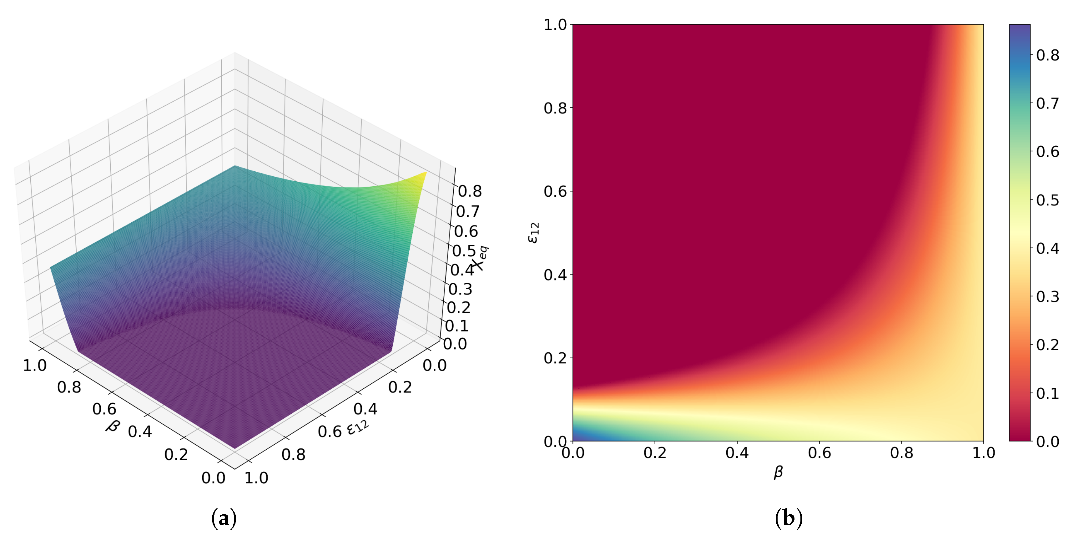
3.3. Directed Degradation and Cooperation in Ribozymes

The next step towards the generalisation of the dynamical system to describe all considered interactions is the addition of density-dependent degradation, describing the process by which some replicators (ribozymes) can degrade the other hypercycle member due to trans-cleaving activity. In order to do so, a new parameter must be introduced, $\beta$, which may be regarded as the fraction of species $S_2$ that receives catalysis from species $S_1$, while $(1-\beta )$ does exactly the opposite with $S_2$ degrading $S_1$ at a rate ${\epsilon }_{12}$. In this case, the cross-catalytic replication for species $S_2$ is affected by the presence of this parameter as only a fraction $\beta$ of this species will receive catalysis.

For the sake of length and simplicity, this section is studied under the assumption that ${\alpha }_1={\alpha }_2={\eta }_{\epsilon }=k=c_0=1$, while $\epsilon ,{\epsilon }_{12},{\eta }_k$ and $\beta$ are allowed to move freely. This lets us focus strictly on the effect of the degradation behaviour led by $S_2$ without over-complicating the whole model. Furthermore, such restrictions have not been chosen arbitrarily but, in fact, hold specific biological meaning and build the cases we are most interested in when considering ribozyme interactions. Hence, the system we will focus on along this section is:

$$\left\{\begin{array}{c}{\dot{x}}_1=(x_1+x_1{x}_2)(1-(x_1+x_2))-\epsilon x_1-(1-\beta ){\epsilon }_{12}{x}_1{x}_2,\hfill \\ {\dot{x}}_2=(x_2+\beta {\eta }_k{x}_1{x}_2)(1-(x_1+x_2))-\epsilon x_2.\hfill \end{array}\right.$$

(23)

An analytical study, as has been carried out in the previous sections, shows that up to three critical points in the first quadrant apart from the origin exist. As previously stated, given ${\alpha }_1={\alpha }_2=1>\epsilon ={\eta }_{\epsilon }\epsilon$, global extinction is impossible since the origin is a repulsive node. As for the other equilibria, one is located on each axis representing the potential survival of a single species without the need of the other. The third equilibrium is only present for a set of values such that ${\eta }_k>0$ and

$$\beta >{\beta }_{\mathrm{bif}}=1-\frac{\epsilon }{{\epsilon }_{12}}>0,$$

(24)

stating that a certain amount of $S_2$ higher than this specific threshold must collaborate with $S_1$ in order to achieve coexistence. Interestingly, for $\epsilon >{\epsilon }_{12}$, both species evolve towards their coexistence regardless of the initial conditions, as long as they are non-zero.

To prove the attractive behaviour of the critical point located outside the axes, we can once again focus on the nullcline distribution. It is quite straightforward to see that bounded to the x-axis, $g\left(x\right)>max\left\{h\right(0\left)\right\}$, where $g\left(x_1\right)$ and $h\left(x_2\right)$ have been defined analogously to the previous sections. This describes the same scenario presented in Figure 3a, which allows us to conclude this equilibrium is stable. The fact that $g\left(x\right)>max\left\{h\right(0\left)\right\}$ on the abscissa tells us that shifting $\beta$ to lower values results in the middle equilibrium to move towards the critical point on the y-axis as long as $\epsilon \le {\epsilon }_{12}$, i.e., ${\beta }_{\mathrm{bif}}\ge 0$, until the critical point leaves the phase space and a transcritical bifurcation takes place ($\beta \le {\beta }_{\mathrm{bif}}$). See Figure 6a,b. On the other hand, if $\epsilon >{\epsilon }_{12}$, lowering $\beta$ results in the approach of the critical point present on the x-axis until $\beta =0$, where they collide and a transcritical bifurcation takes place as well. See Figure 6c,d.

Finally, a different behaviour is seen for ${\eta }_k=0$, i.e., when $S_2$ is unable to catalytically replicate with the help of $S_1$. In this case, there are only three critical points in the region of interest: the origin, which remains a repulsive node, and each individual survival. If $\beta >{\beta }_{\mathrm{bif}}$, then the previous critical point approaches the equilibrium on the $x-$axis as ${\eta }_k$ is reduced until it reaches zero and is absorbed by it. However, for $\beta <{\beta }_{\mathrm{bif}}$, it is the other equilibrium that becomes the $\omega -$limit of the system. See Figure 6e and Figure 6f, respectively.

The behaviour described above can be very well visualised by plotting three-dimensional and heatmap bifurcation diagrams where the $x_1^{*}$ or $x_2^{*}$ equilibrium component is computed for given parameters. This is possible given the fact that all orbits outside the axes will evolve to the same equilibrium point and because the origin acts as a repulsive node at all times. Thus, if we choose to plot $x_1^{*}$, i.e., the abscissa component of the equilibrium, and it falls on 0, we can read that $S_1$ has been extinguished, while $S_2$ has survived. The annihilation of $S_2$ when ${\eta }_k>0$ is only possible for $\epsilon >{\epsilon }_{12}$ and $\beta =0$; therefore, it is more adequate to represent $x_1^{*}$ instead of $x_2^{*}$ as the coexistence will be present as long as $x_1^{*}>0$ and $\beta \ne 0$.

Keeping this argument in mind, Figure 7 collects all information presented in Figure 6a–c. Indeed, we can see how the coexistence is present for $\beta >{\beta }_{\mathrm{bif}}$, while $S_1$ ceases to exist if $\beta \le {\beta }_{\mathrm{bif}}$. For ${\eta }_k=0$, Figure 8 shows how $x_1^{*}$ becomes zero if $\beta <{\beta }_{\mathrm{bif}}$, indicating that $S_1$ vanishes while $S_2$ remains, and vice versa for $\beta >{\beta }_{\mathrm{bif}}$. In order to demonstrate that coexistence is not possible in these scenarios, both $x_1^{*}$ and $x_2^{*}$ have been represented in separate plots (Figure 8a,c and Figure 8b,d, respectively). Note that the coexistence that can be observed on the curve $\beta ={\beta }_{\mathrm{bif}}$ is not a mere casualty and is thoroughly explained below.

As presented in Figure 8, the case $\beta ={\beta }_{\mathrm{bif}}$ under ${\eta }_k=0$ is quite interesting as well. Here, both equilibria located on the axes are present; hence, the nullclines become the exact same curves in the phase space. This translates to a continuum of fixed points filling the attractive linear manifold $x_2=1-\epsilon -x_1$. The dynamical system under these conditions and the adequate simplification becomes:

$$\left\{\begin{array}{c}{\dot{x}}_1=-x_1(x_2+1)(x_1+x_2+\epsilon -1),\hfill \\ {\dot{x}}_2=-x_2(x_1+x_2+\epsilon -1).\hfill \end{array}\right.$$

(25)

Assuming $(x_1+x_2+\epsilon -1)\ne 0$, we can compute the quotient ${\dot{x}}_1/{\dot{x}}_2$, allowing us to find a first integral of the problem:

$$\frac{{\dot{x}}_1}{{\dot{x}}_2}=\frac{x_1(x_2+1)}{x_2}\Rightarrow \frac{{\dot{x}}_1}{x_1}=\left(1+\frac{1}{x_2}\right){\dot{x}}_2,$$

(26)

integrating on both sides, we obtain

$$ln\left(x_1\right)=x_2+ln\left(x_2\right)+C,$$

(27)

such that if initial conditions $x_1\left(0\right),x_2\left(0\right)$ are the species initial conditions, Equation (27) can be rewritten as

$$x_1=\frac{x_1\left(0\right)}{x_2\left(0\right)}{x}_2{e}^{x_2-x_2\left(0\right)}.$$

(28)

Taking $H=ln\left(x_1\right)-x_2-ln\left(x_2\right)=0$ and X the system’s field, we have

$$H^{\prime }=〈\nabla H,X〉=\frac{\dot{x_1}}{x_1}-\left(1+\frac{1}{x_2}\right){\dot{x}}_2=0$$

(29)

which confirms that the expression is a first integral. This result tells us that all orbits outside the axes follow Equation (27) until they reach the stable line $x_2=1-\epsilon -x_1$. This is of course attractive since ${\dot{x}}_1,{\dot{x}}_2>0$ for $x_1+x_2<1-\epsilon$ and ${\dot{x}}_1,{\dot{x}}_2<0$ for $x_1+x_2>1-\epsilon$. The corresponding phase portrait for this setting is shown in Figure 9, where the solutions can be seen to follow exactly the level curves of the first integral.

Interestingly enough, we are in front of a case of extreme equilibrium in which the degrading species, $S_2$, is unable to cross-catalytically replicate with $S_1$, while $S_1$ benefits from this interaction with a fraction $\beta$ of $S_2$ but is degraded by a fraction $1-\beta$.

Another case worth considering is that in which $\epsilon =0$ and ${\epsilon }_{12}\ll 1$, meaning that natural degradation is no longer present. This leaves us with a system in which both species will only decrease as a consequence of the coupling term as long as $x_1+x_2>1$. For ${\epsilon }_{12}=0$, the ODE system (1) becomes:

$$\left\{\begin{array}{c}{\dot{x}}_1=(x_1+x_1{x}_2)(1-(x_1+x_2)),\hfill \\ {\dot{x}}_2=(x_2+\beta {\eta }_k{x}_1{x}_2)(1-(x_1+x_2)).\hfill \end{array}\right.$$

(30)

These equations can be solved assuming $1-(x_1+x_2)\ne 0$, dividing ${\dot{x}}_1$ over ${\dot{x}}_2$, and organising both sides of the expression to find:

$$\left(\beta {\eta }_k+\frac{1}{x_1}\right){\dot{x}}_1=\left(1+\frac{1}{x_2}\right){\dot{x}}_2,$$

(31)

which can be integrated resulting in

$$\beta {\eta }_k{x}_1+ln\left(x_1\right)=x_2+ln\left(x_2\right)+C,$$

(32)

where $C=\beta {\eta }_k{x}_1\left(0\right)+ln\left(x_1\left(0\right)\right)-x_2\left(0\right)-ln\left(x_2\left(0\right)\right)$. This curve describes the orbits followed by an initial condition $(x_1\left(0\right),x_2\left(0\right))$ in the phase space such that $1-(x_1\left(0\right)+x_2\left(0\right))\ne 0$. Note that $1-(x_1+x_2)=0$ is a continuum of attractive equilibria and that the origin acts as a repulsive node. Figure 9b explicitly shows this behaviour. Finally, as long as $\beta >0$, a small variation in ${\epsilon }_{12}$ brings us straight to the case studied in Figure 6b, implying the extinction of $S_1$, and a minor variation in $\epsilon$ recovers Figure 6c, showing coexistence.

3.4. Interplay between Predation and Cooperation in Ecology

All systems studied above have been analysed in order to build up a general hypercycle model that allows us to consider all interactions presented in Section 3.3 while $S_2$ also behaves as a predator. Both species are now under the influence of self-replication (${\alpha }_i>0$ for $i=1,2$) and cross-catalytic replication ($k,{\eta }_k>0$), they are also degraded by natural causes ($\epsilon ,{\eta }_{\epsilon }>0$), a fraction $\beta$ of $S_2$ receives cooperation from $S_1$, the rest of $S_2$ ($1-\beta$) consumes $S_1$ at a rate ${\epsilon }_{12}$, and for the first time, $S_2$ benefits from this consumption with an efficiency of $\gamma \in (0,1)$, acting as a predator. We now reached the system presented in Equation (1), Section 2, with all parameters playing their corresponding biological roles:

$$\left\{\begin{array}{c}{\dot{x}}_1=({\alpha }_1{x}_1+k{x}_1{x}_2)(1-(x_1+x_2))-\epsilon x_1-(1-\beta ){\epsilon }_{12}{x}_1{x}_2,\hfill \\ {\dot{x}}_2=({\alpha }_2{x}_2+\beta {\eta }_{k}k{x}_1{x}_2)(1-(x_1+x_2))-{\eta }_{\epsilon }\epsilon x_2+\gamma (1-\beta ){\epsilon }_{12}{x}_1{x}_2.\hfill \end{array}\right.$$

(33)

As we did above, we shall consider a simple scenario setting ${\alpha }_1={\alpha }_2=k={\eta }_{\epsilon }=c_0=1$ to be able to analyse it mathematically and to obtain clearer results arising from predation. Even though a new process is being considered in this case, surprisingly, the dynamics of the predatory scenario behave exactly as those described in Section 3.3. Curiously enough, although species $S_2$ now grows at the expense of $S_1$, studying the relative positions of the nullclines shows that for $\beta >{\beta }_{\mathrm{bif}}=1-\epsilon /{\epsilon }_{12}$, there is coexistence while $S_1$ vanishes for $\beta \le {\beta }_{\mathrm{bif}}$ (see Figure 10 and Figure 11). As previously explained, the existence of the coexistence equilibrium is given by the position of all four positive axis crossings of the nullclines. We shall refer to the intersection of the $x_j$ nullcline with the $x_i-$axis as $x_{i,j}^{*}$ and claim that $x_{1,1}^{*}<x_{1,2}^{*}$ and $x_{2,1}^{*}>x_{2,2}^{*}$ for $\beta >{\beta }_{\mathrm{bif}}$, which implies the desired coexistence. Let us compute these values explicitly. On the $x_1$ axis, the intersections of interest happen at

$$\begin{array}{cc}\hfill x_{1,1}^{*}& =1-\epsilon ,\hfill \\ \hfill x_{1,2}^{*}& =\frac{1}{2\beta {\eta }_k}\left(-\beta \gamma {\epsilon }_{12}+\beta {\eta }_k+{\epsilon }_{12}\gamma -1+\sqrt{{(-\beta \gamma {\epsilon }_{12}+\beta {\eta }_k+{\epsilon }_{12}\gamma -1)}^2+4\beta {\eta }_k(1-\epsilon )}\right),\hfill \end{array}$$

(34)

for ${\dot{x}}_1=0$ and ${\dot{x}}_2$, respectively. These values will coincide if

$$\beta =\frac{{\epsilon }_{12}\gamma }{{\epsilon }_{12}\gamma -\epsilon {\eta }_k},$$

(35)

which is greater than 1, positive for ${\epsilon }_{12}\gamma >\epsilon {\eta }_k$, and negative for ${\epsilon }_{12}\gamma <\epsilon {\eta }_k$. Notice that the change of sign implies a change in the inequality such that for the considered range of $\beta$, it can only be that $x_{1,1}^{*}<x_{1,2}^{*}$. This is precisely the reason behind the non-alteration of the dynamics under predatory behaviour. On the vertical axis, the crossings are given by

$$\begin{array}{cc}\hfill x_{2,1}^{*}& =\frac{1}{2}\left(-{\epsilon }_{12}(1-\beta )+\sqrt{{\epsilon }_{12}^2{(1-\beta )}^2+4(1-\epsilon )}\right),\hfill \\ \hfill x_{2,2}^{*}& =1-\epsilon .\hfill \end{array}$$

(36)

In this case, $x_{2,1}^{*}=x_{2,2}^{*}$ occurs at the critical value

$$\beta =1-\frac{\epsilon }{{\epsilon }_{12}}={\beta }_{\mathrm{bif}},$$

(37)

and $x_{2,1}^{*}>x_{2,2}^{*}$ for $\beta >{\beta }_{\mathrm{bif}}$, a value that can very well be assumed by $\beta$. Thus, the claim follows, and we conclude that a dual behaviour within $S_2$ concerning its interaction with $S_1$ does not modify the overall dynamics of the system. As expected, all equilibria are found at values of $S_2$ just above those studied in the preceding section since $S_2$ is now replicating from the extinction of $S_1$. Moreover, the results found for $\beta ={\beta }_{\mathrm{bif}}$ are now independent of ${\eta }_k$ as the influence of $\gamma$ on the system makes coexistence impossible under such assumptions (see Figure 11a). Of course, since $\gamma$ multiplies ${\epsilon }_{12}$ in ${\dot{x}}_2$, considering $\epsilon ={\epsilon }_{12}=0$ brings us to the same results shown in Equation (32) and small perturbation of ${\epsilon }_{12}$ will also result in the $S_1$ to extinction given $\gamma {\epsilon }_{12}>0$ (see Figure 11b).

4. Conclusions

Research on hypercycles has focused on the dynamics arising from the processes of cooperation (e.g., catalysis) between replicators [3,53,54,55,56]. The cyclic architecture of cooperative interactions is known to provide stability and survival of all the species. However, other different architectures able to impair such stability have been thoroughly investigated. These include the so-called catalytic parasites [15,57,58,59,60] and the catalytic short-circuits [61,62]. Recent research has combined cooperative interactions with other antagonistic processes between species [63]. This is based on the rationale that molecular replicators are subject to mutational processes and ecological species to behavioural shifts due to environmental or ecological changes. These changes could make species switch from cooperative to antagonistic interactions, in, what we have called here, a functional shift. These functional shifts could arise in ribozymes due to mutational processes and could involve a shift from cooperation (hetero-catalysis) to directed degradation (trans-cleavage) [63]. In the context of complex ecosystems, several species undergoing inter-specific cooperation are known to switch to predation (see for example Refs. [65,66,67,68]). Even though the drivers of such functional shifts may not be trivial and respond to complex behavioural patterns among species or both biotic and abiotic changes, the dynamics arising due to such functional shifts are still an unexplored subject. As mentioned, some authors have used the hypercycle theory to investigate the impact of these functional shifts in ecosystems dynamics [63]. Specifically, the impact of a shift from catalytic cooperation to directed degradation was studied in small (one to four species) discrete-time hypercycles [63]. As far as we know, no works have investigated how these shifts may affect the stability of small hypercycles in time-continuous systems.

In this article, we have analysed two-species hypercycles considering, together with cooperation, directed degradation or predation (see Figure 1). The changes due to functional shifts have been studied using a general hypercycle model that allows for different architectures by changing different parameter conditions. To understand the changes due to these functional shifts, we have summarised and extended previous results on obligate two-member hypercycles [53] while also analysing a facultative case.

The model considering directed degradation shows no full extinction when both autocatalytic replication rates are higher than their natural decays. We have found a critical value for $\beta$, ${\beta }_{\mathrm{bif}}$, below which only the dominant species $S_2$ survives, while coexistence is present for $\beta >{\beta }_{\mathrm{bif}}$. We have also identified parametric scenarios (i.e., considering no catalytic support of the degrader species by the other one (${\eta }_k=0$) or no decay rate of any of the two species ($ϵ=0$)), giving place to a continuum of fixed critical points following a straight line at $\beta ={\beta }_{\mathrm{bif}}$. For these two scenarios, the complete analytical expressions describing all orbits have been found. Finally, we considered a cooperative system with predation. Interestingly, bifurcation parameters found for the directed degradation system re-appeared in the same form, stating that no natural benefit towards $S_2$ is enough to change the dynamics of the system as long as ${\eta }_k\epsilon >0$. However, these extreme cases with ${\eta }_k=0$ or $ϵ=0$ stopped presenting a continuum of critical points and turned into the extinction of $S_1$ as a consequence of the predatory term.

Future research directions may consider functional shifts in non-autonomous systems, considering that changes among cooperative and antagonistic interactions may vary in time due to seasonality or external perturbations.

References

1. Eigen, M. Selforganization of matter and the evolution of biological macromolecules. Die Naturwissenschaften 1971, 58, 465–523. [Google Scholar] [CrossRef] [PubMed]
2. Müller-Herold, U. What is a hypercycle? J. Theor. Biol. 1983, 102, 569–584. [Google Scholar] [CrossRef]
3. Eigen, M.; Schuster, P. The Hypercycle: A Principle of Natural Selforganization; Springer: Berlin, Germany, 1979. [Google Scholar]
4. Kauffman, S. The Origins of Order: Self-Organization and Selection in Evolution; Oxford University: Oxford, UK, 1993. [Google Scholar]
5. Eigen, M.; Biebricher, C.K.; Gebinoga, M.; Gardiner, W.C. The hypercycle. Coupling of RNA and protein biosynthesis in the infection cycle of an RNA bacteriophage. Biochemistry 1991, 30, 11005–11018. [Google Scholar] [CrossRef]
6. Szathmáry, E. Natural selection and dynamical coexistence of defective and complementing virus segments. J. Theor. Biol. 1992, 157, 383–406. [Google Scholar] [CrossRef]
7. Szathmáry, E. Co-operation and defection: Playing the field in virus dynamics. J. Theor. Biol. 1993, 165, 341–356. [Google Scholar] [CrossRef]
8. Sardanyés, J.; Elena, S.F. Error threshold in RNA quasispecies models with complementation. J. Theor. Biol. 2010, 265, 278–286. [Google Scholar] [CrossRef] [Green Version]
9. Cohen, M.A.; Grossberg, S. Absolute stability and global pattern formation and parallel memory storage by competitive neural networks. IEEE Trans. Syst. Man Cybern. 1983, 13, 815–826. [Google Scholar] [CrossRef]
10. Cohen, M.A.; Grossberg, S. Pattern Recognition by Self-Organizing Neural Networks; MIT Press: Cambridge, MA, USA, 1991. [Google Scholar]
11. Farmer, J.D.; Kauffman, S.A.; Packard, N.H.; Perelson, A.S. Adaptive dynamic networks as models for the immune system and autocatalytic sets. In Perspectives in Biological Dynamics and Theoretical Medicine; Annals of the New York Academy of Sciences: New York, NY, USA, 1987. [Google Scholar]
12. Nowak, M.A.; Krakauer, D.C. The evolution of language. Proc. Natl. Acad. Sci. USA 1999, 96, 8028–8033. [Google Scholar] [CrossRef] [Green Version]
13. Lee, D.H.; Severin, K.; Ghadiri, M.R. Autocatalytic networks: The transition from molecular self-replication to molecular ecosystems. Curr. Opin. Chem. Biol. 1997, 1, 491–496. [Google Scholar] [CrossRef]
14. Shou, W.; Ram, S.; Vilar, J.M.G. Synthetic cooperation in engineered yeast populations. Proc. Natl. Acad. Sci. USA 2007, 104, 1877–1882. [Google Scholar] [CrossRef] [PubMed] [Green Version]
15. Amor, D.R.; Montañez, R.; Duran-Nebreda, S.; Solé, R. Spatial dynamics of synthetic microbial mutualists and their parasites. PLoS Comput. Biol. 2017, 13, e15689. [Google Scholar] [CrossRef] [Green Version]
16. Stadler, B.; Stadler, P. Molecular replicator dynamics. Adv. Complex Syst. 2003, 6, 47–77. [Google Scholar] [CrossRef] [Green Version]
17. Niesert, U.; Harnasch, D.; Bresch, C. Origin of life between Scylla and Charybdis. J. Mol. Evol. 1981, 17, 348–353. [Google Scholar] [CrossRef] [PubMed]
18. Usher, D.A.; McHale, A.H. Hydrolyitc stability of helical RNA: A selective advantage for the natural 3’, 5’-bond. Proc. Natl. Acad. Sci. USA 1976, 73, 1149–1153. [Google Scholar] [CrossRef] [Green Version]
19. Lohrmann, R.; Orgel, L.E. Self-condensation of activated dinucleotides on polynucleotide templates with alternating sequences. J. Mol. Evol. 1979, 14, 243–250. [Google Scholar] [CrossRef]
20. Cech, T.R. The chemistry of self-replicating RNA and RNA enzymes. Science 1987, 236, 1532–1539. [Google Scholar] [CrossRef] [PubMed]
21. Kruger, K.; Grabowski, P.J.; Zaug, A.J.; Sands, J.; Gottschling, D.E.; Cech, T.R. Self-splicing RNA: Autoexcision and autocyclization of the ribosomal RNA intervening sequence of Tetrahymena. Cell 1982, 31, 147–157. [Google Scholar] [CrossRef]
22. Daròs, J.A. Eggplant latent viroid: A friendly experimental system in the family Asunviroidae. Mol. Plant Pathol. 2016, 17, 1170–1177. [Google Scholar] [CrossRef] [Green Version]
23. Vlassov, A.V. Mini-ribozymes and freezing environment: A new scenario for the early RNA world. Biogeosci. Discuss. 2005, 2, 1719–1737. [Google Scholar]
24. Robertson, M.P.; Joyce, G.F. The origins of the RNA world. Cold Spring Harb. Perspect. Biol. 2012, 4, a003608. [Google Scholar] [CrossRef]
25. Neveu, M.; Kim, H.J.; Benner, S.A. The strong RNA world hypothesis: Fifty years old. Astrobiology 2013, 13, 391–403. [Google Scholar] [CrossRef] [Green Version]
26. Doudna, J.A.; Cech, T.R. The chemical repertoire of natural ribozymes. Nature 2002, 418, 222–228. [Google Scholar] [CrossRef]
27. Zhang, B.; Cech, T.R. Peptidyl-transferase ribozymes: Trans reactions, structural characterization and ribosomal RNA-like features. Chem. Biol. 1998, 5, 539–553. [Google Scholar] [CrossRef] [Green Version]
28. Been, M.D.; Barford, E.T.; Burke, J.M.; Price, J.V.; Tanner, N.K.; Zaug, A.J.; Cech, T.R. Structures involved in Tetrahymena rRNA self-splicing and RNA enzyme activity. Cold Spring Harb. Symp. Quant. Biol. 1987, 52, 147–157. [Google Scholar] [CrossRef] [PubMed]
29. Zielinksi, W.S.; Orgel, L.E. Oligomerization of activated derivatives of 3’-amino-3’-deoxyguanosine on poly(C) and poly(dC) template. Nucl. Acid Res. 1985, 13, 8999–9009. [Google Scholar]
30. Von Kiedrowski, G. A self-replicating hexadeoxynucleotide. Angew. Chem. Int. Ed. 1986, 119, 932–935. [Google Scholar] [CrossRef]
31. Jimenez, R.M.; Polanco, J.A.; Lupták, A. Chemistry and biology of self-cleaving ribozymes. Trends Biochem. Sci. 2015, 40, 648–661. [Google Scholar] [CrossRef] [PubMed] [Green Version]
32. Carbonell, A.; Flores, R.; Gago, S. Trans-cleaving hammerhead ribozymes with tertiary stabilizing motifs: In vitro and in vivo activity against a structured viroid RNA. Nucl. Acid Res. 2011, 39, 2432–2444. [Google Scholar] [CrossRef]
33. Weinberg, C.E.; Weinberg, Z.; Hammann, C. Noverl ribozymes: Discovery, catalytic mechanisms, and the quest to understand biological functions. Nucl. Acid Res. 2019, 47, 9480–9494. [Google Scholar] [CrossRef]
34. Weinberg, C.E.; Weinberg, Z.; Hammann, C. In-ice evolution of RNA polymerase ribozyme activity. Nature Chem. 2013, 5, 1011–1018. [Google Scholar]
35. Vaidya, N.; Manapat, M.L.; Chen, I.A.; Xulvi-Brunet, R.; Hayden, E.J.; Lehman, N. Spontaneous network formation among cooperative RNA replicators. Nature 2002, 491, 72–77. [Google Scholar] [CrossRef]
36. Smith, J.M.; Szathmáry, E. The Major Transitions in Evolution; Oxford University Press: Oxford, UK, 1995. [Google Scholar]
37. Sardanyés, J. The hypercycle: From molecular to ecosystems dynamics. In Landscape Ecology Research Trend; Nova Publishers: Hauppauge, NY, USA, 2009. [Google Scholar]
38. Dugatkin, L.A. Cooperation Among Animals. An Evolutionary Perspective; Dugatkin, L.A., Ed.; Oxford Series in Ecology and Evolution; Oxford University Press: New York, NY, USA, 1997; pp. 90–115. [Google Scholar]
39. Packer, C.; Ruttan, L. The evolution of cooperative hunting. Am. Nat. 1988, 132, 159–198. [Google Scholar] [CrossRef]
40. Cordes, E.E.; Arthur, M.A.; Shea, K.; Arvidson, R.S.; Fisher, C.R. Modeling the Mutualistic Interactions between Tubeworms and Microbial Consortia. PLoS Biol. 2005, 3, e77. [Google Scholar] [CrossRef] [Green Version]
41. van Schaik, C.P.; Kappeler, P.M. Cooperation in Primates and Humans. Mechanisms of Evolution; Kappeler, P.M., van Schaik, C.P., Eds.; Springer: New York, NY, USA, 2006; pp. 4–21. [Google Scholar]
42. Smith, S.E.; Read, D.J. Mycorrhizal Symbiosis; Academic: New York, NY, USA, 1996. [Google Scholar]
43. McNab, B.K. Energetics and the distribution of vampires. J. Mammol. 1973, 54, 131–144. [Google Scholar] [CrossRef]
44. Wilkinson, G. Reciprocal food sharing in vampire bats. Nature 1984, 308, 181–184. [Google Scholar] [CrossRef]
45. Wilkinson, G. The social organization of the common vampire bat. II. Mating systems, genetic structure and relatedness. Behav. Ecol. Sociobiol. 1985, 17, 123–134. [Google Scholar]
46. Stander, P.E. Cooperative hunting in lions: The role of the individual. Behav. Ecol. Sociobiol. 1992, 29, 445–454. [Google Scholar] [CrossRef]
47. Mills, M.G.L. Foraging behaviour of the brown hyaena (Hyaena brunnea Thunberg, 1820) in the southern Kalahari. Z. Tierpsychol. 1978, 48, 113–141. [Google Scholar] [CrossRef]
48. Boesch, C.; Boesch, H.; Vigilant, L. Cooperative hunting in chimpanzees: Kinship or mutualism? In Cooperation in Primates and Humans: Mechanisms and Evolution; Springer: Berlin/Heidelberg, Germany, 2006; pp. 139–150. [Google Scholar]
49. Major, P.F. Predator-Prey Interactions in Two Schooling Fishes, Caranx ignobilis and Stolephorus purpureus. Anim. Behav. 1978, 26, 760–777. [Google Scholar] [CrossRef]
50. Rypstra, A.L. Aggregations of Nephila clavipes (L.) (Araneae, Araneidae) in Relation to Prey Availability. J. Arachnol. 1985, 13, 71–78. [Google Scholar]
51. Ward, P.I.; Enders, M.M. Conflict and cooperation in the group feeding of the social spider Stegodyphus mimosarum. Behaviour 1985, 94, 167–182. [Google Scholar]
52. Nakasuji, F.; Dyck, V.A. Evaluation of the role of Microvelia douglasi atrolineata (Bergroth) (Hemiptera: Veliidae) as predator of the brown planthopper, Nilaparvata lugens (Stal) (Homoptera: Delphacidae). Res. Pop. Ecol. 1984, 26, 148–163. [Google Scholar] [CrossRef]
53. Sardanyés, J.; Solé, R.V. Bifurcations and phase transitions in spatially extended two-member hypercycles. J. Theor. Biol. 2006, 243, 468–482. [Google Scholar] [CrossRef] [PubMed] [Green Version]
54. Sardanyés, J. Error threshold ghosts in a simple hypercycle with error prone self-replication. Chaos Solitons Fractals 2008, 35, 313–319. [Google Scholar] [CrossRef]
55. Silvestre, D.A.M.M.; Fontanari, J.F. The information capacity of hypercycles. J. Theor. Biol. 2008, 254, 804–806. [Google Scholar] [CrossRef] [Green Version]
56. Guillamon, A.; Fontich, E.; Sardanyés, J. Bifurcations analysis of oscillating hypercycles. J. Theor. Biol. 2015, 387, 23–30. [Google Scholar] [CrossRef] [PubMed] [Green Version]
57. Boerlijst, M.C.; Hogeweg, P. Spiral wave structure in prebiotic evolution: Hypercycles stable against parasites. Phys. D 1991, 48, 17–28. [Google Scholar] [CrossRef]
58. Boerlijst, M.C.; Hogeweg, P. Spatial gradients enhance persistence of hypercycles. Phys. D 1995, 88, 29–39. [Google Scholar] [CrossRef] [Green Version]
59. Cronhjort, M.B. Cluster compartmentalization may provide resistance to parasites for catalytic networks. Phys. D 1997, 101, 289–298. [Google Scholar] [CrossRef]
60. Sardanyés, J.; Solé, R.V. Spatio-temporal dynamics in simple asymmetric hypercycles under weak parasitic coupling. Phys. D 2007, 231, 116–129. [Google Scholar] [CrossRef]
61. Kim, P.J.; Jeong, H. Spatio-temporal dynamics in the origin of genetic information. Phys. D 2005, 203, 88–99. [Google Scholar] [CrossRef] [Green Version]
62. Sardanyés, J.; Lázaro, J.T.; Guillamon, A.; Fontich, E. Full analysis of small hypercycles with short-circuits in prebiotic evolution. Phys. D 2017, 34, 90–108. [Google Scholar] [CrossRef]
63. Perona, J.; Fontich, E.; Sardanyés, J. Dynamical effects of loss of cooperation in discrete-time hypercycles. Phys. D 2020, 406, 132425. [Google Scholar] [CrossRef]
64. Scott, M.D.; Chivers, S.J.; Olson, R.J.; Holland, K. Pelagic predator associations: Tuna and dolphins in the eastern tropical Pacific Ocean. Mar. Ecol. Prog. Ser. 2012, 458, 283–302. [Google Scholar] [CrossRef]
65. Maldini, D. Evidence of predation by a tiger shark (Galeocerdo cuvier) on a spotted dolphin (Stenella attenuata) off Oahu, Hawaii. Aquat. Mamm. 2003, 29, 84–87. [Google Scholar] [CrossRef]
66. Melillo-Sweeting, K.; Turnbull, S.D.; Guttridge, T.L. Evidence of shark attacks on Atlantic spotted dolphins (Stenella frontalis) off Bimini, The Bahamas. Mar. Mammal Sci. 2014, 30, 1158–1164. [Google Scholar] [CrossRef]
67. Votier, S.C.; Furness, R.W.; Bearhop, S.; Crane, J.E.; Caldow, R.W.G.; Catry, P.; Ensor, K.; Hamer, K.C.; Hudson, A.V.; Kalmbach, E.; et al. Changes in fisheries discard rates and seabird communities. Nature 2004, 427, 727–730. [Google Scholar] [CrossRef]
68. Almaraz, P.; Oro, D. Size-mediated non-trophic interactions and stochastic predation drive assembly and dynamics in a seabird community. Ecology 2011, 92, 1948–1958. [Google Scholar] [CrossRef] [PubMed]
69. Hatch, J.J. Predation and piracy by gulls at a ternery in Maine. Auk 1970, 87, 244–254. [Google Scholar] [CrossRef]
70. Andersson, M. Predation and kleptoparasitism by skuas in a Shetland seabird colony. Ibis 1976, 118, 208–217. [Google Scholar] [CrossRef]
71. Götmark, F.; Andersson, M. Breeding Association between Common Gull Larus canus and Arctic Skua Stercorarius parasiticus. Ornis Scand. 1980, 11, 121–124. [Google Scholar] [CrossRef]
72. Oro, D. Interspecific kleptoparasitism in Audouin’s Gull Larus audouinii at the Ebro Delta, northeast Spain: A behavioural response to low food availability. Ibis 1996, 138, 218–221. [Google Scholar] [CrossRef]
73. Oro, D. Breeding Biology and Population Dynamics of Slender-billed Gulls at the Ebro Delta (Northwestern Mediterranean). Waterbirds 2002, 25, 67–77. [Google Scholar] [CrossRef]
74. Sadoul, N.; Johnson, A.R.; Walmsley, J.; Levéque, R. Changes in the numbers and the distribution of colonial Charadriifromes breeding in the Camargue, Southern France. Col. Waterbirds 1996, 19, 46–58. [Google Scholar] [CrossRef]
75. Martínez-Abraín, A.; Genovart, M.; Oro, D. Kleptoparasitism, disturbance and predation of yellow-legged gulls on Audouin’s gulls in three colonies of the Western Mediterranean. Sci. Mar. 2003, 67, 89–94. [Google Scholar] [CrossRef] [Green Version]
76. Guinet, C.; Bouvier, J. Development of intentional stranding hunting techniques in killer whale (Orcinus orca) calves at Crozet Archipelago. Can. J. Zool. 1995, 73, 27–33. [Google Scholar] [CrossRef]
77. Sardanyés, J.; Solé, R. Ghosts in the origins of life? Int. J. Bifurc. Chaos 2006, 16, 2761–2765. [Google Scholar] [CrossRef]
78. García-Tejedor, A.; Morán, F.; Montero, F. Influence of the Hypercyclic Organization on the Error Threshold. J. Theor. Biol. 1987, 127, 393–402. [Google Scholar] [CrossRef]
79. García-Tejedor, A.; Sanz-Nuño, J.C.; Olarrea, J.; de la Rubia, F.J.; Montero, F. Influence of the Hypercycle on the Error Threshold: A Stochastic Approach. J. Theor. Biol. 1988, 134, 431–443. [Google Scholar] [CrossRef]
80. Nuño, J.C.; Montero, F.; de la Rubia, F.J. Influence of external fluctuations on a hypercycle formed by two kinetically indistinguishable species. J. Theor. Biol. 1993, 165, 553–575. [Google Scholar] [CrossRef]
Figure 1. The different hypercycle architectures studied in this article: (a) obligate two-species hypercycle with heterocatalysis; (b) facultative system with heterocatalysis and autonomous self-replication; (c) hypercycle including directed degradation of S 1 by S 2 while still keeping some fractions of the population receiving catalytic aid; (d) two-species ecological hypercycle (e.g., wader and seagull) including opportunistic predation (especially on eggs and chicks). Here, S 2 consumes S 1 , while some individuals still receive cooperation from S 1 .
Mathematics 09 01809 g001
Figure 2. Possible dynamical scenarios according to the shape of the nullclines. Solutions of x ˙ 1 = 0 are plotted in black and in red for x ˙ 2 = 0 . The symmetry coefficients η k and η ε have been set to 1 for the three plots.
Mathematics 09 01809 g002
Figure 3. The direction of the dynamical system vector field for all possible situations regarding ε < α 1 , α 2 / η ε together with nullclines g ( x 2 ) and h ( x 1 ) plotted in black and red, respectively. Parameters used: (a) ε = 0.16 , k = 0.74 , α 1 = 0.28 , α 2 = 0.4 ; (b) ε = 0.17 , k = 0.59 , α 1 = 0.96 , α 2 = 0.27 ; (c) ε = 0.17 , k = 0.40 , α 1 = 0.28 , α 2 = 0.78 . Below, we display all possible phase portraits for the two-member hypercycle with exponential replication parameter higher than its decay rate in both species. In particular, the plots have been obtained for the values: (a) α 1 = 0.39 , α 2 = 0.94 , ε = 0.14 , k = 1 , η k = 3.6 , η ε = 2.95 ; (b) α 1 = 0.77 , α 2 = 0.51 , ε = 0.14 , k = 0.28 , η k = 3.6 , η ε = 2.95 ; (c) α 1 = 0.27 , α 2 = 0.93 , ε = 0.16 , k = 0.3 , η k = 0.35 , η ε = 1.45 . Stable equilibria are denoted with red solid circles.
Mathematics 09 01809 g003
Figure 4. The direction of the dynamical system vector field for all possible situations regarding α 1 > ε and α 2 < η ε ε . Below, we display a phase portrait of the system in the five possible situations studied. Specifically, the plots have been obtained using the following parameters: (a) α 1 = 0.3 , α 2 = 0.18 , ε = 0.23 , k = 0.29 , η k = 5.5 , η ε = 2.3 ; (b) α 1 = 0.24 , α 2 = 0.05 , ε = 0.21 , k = 0.37 , η k = 4.3 , η ε = 1.2 ; (c) α 1 = 0.34 , α 2 = 0.13 , ε = 0.32 , k = 1 , η k = 7.5 , η ε = 2.75 ; (d) α 1 = 0.56 , α 2 = 0.13 , ε = 0.32 , k = 1 , η k = 7.5 , η ε = 2.75 ; (e) α 1 = 0.86 , α 2 = 0.14 , ε = 0.17 , k = 0.29 , η k = 7.5 , η ε = 2.75 .
Mathematics 09 01809 g004
Figure 5. (Left) A bifurcation diagram when ε > ( k η k + α 2 ) 2 / ( 4 η k η ε k ) using α 1 ( ε , 1 ) as control parameter for a set of parameters such that the four cases in Figure 4b–e are present. Specifically, α 2 = 0.14 , ε = 0.26 , k = 1 , η k = 2.75 , η ε = 2.25 . Stable equilibria are represented in blue for x 1 * and in red for x 2 * coordinates. (Right) Close up of the diagram for α 1 ( α 1 c , α 1 ) showing the coexistence of two stable equilibria; one of which implies the extinction of x 2 .
Mathematics 09 01809 g005
Figure 6. Phase portraits of the system in the qualitatively different identified situations. Specifically, we have used: (a) ε = 0.13 , ε 12 = 0.72 , β = 0.9 , η k = 1.7 ; (b) ε = 0.13 , ε 12 = 0.72 , β = 0.25 , η k = 1.7 ; (c) ε = 0.52 , ε 12 = 0.22 , β = 0.55 , η k = 0.8 ; (d) ε = 0.52 , ε 12 = 0.22 , β = 0 , η k = 0.8 ; (e) ε = 0.25 , ε 12 = 0.49 , β = 0.8 , η k = 0 ; (f) ε = 0.25 , ε 12 = 0.49 , β = 0.14 , η k = 0 . Again, a red dot indicates the ω limit of each orbit and a blue dot its initial condition.
Mathematics 09 01809 g006
Figure 7. Two-parameter bifurcation diagram representing x 1 * as a function of ε 12 and β plotted as a surface (a) and as a heat map (b) for a more intuitive understanding. Parameters used: ε = 0.2 , η k = 2 .
Mathematics 09 01809 g007
Figure 8. Two-parameter bifurcation diagram representing x 1 * (a,c) and x 2 * (b,d) as a function of ε 12 and β plotted as a surface (a,b) and a heat map (c,d) for a more intuitive understanding. Parameters used: ε = 0.13 , η k = 0 .
Mathematics 09 01809 g008
Figure 9. Phase portraits showing a continuum of equilibrium points following x 1 + x 2 = 1 ε (line of quasi-neutral equilibria). Initial conditions are represented with a blue dot and their ω limit with a red dot. Specific parameters used are: (a) ε = 0.25 , ε 12 = 0.49 , η k = 0 , and β = β bif = 0.8194 ; and (b) ε = 0 , ε 12 = 0 , η k = 0.8 , and β = 0.5 .
Mathematics 09 01809 g009
Figure 10. Two-parameter bifurcation diagram representing x 1 * as a function of ε 12 and β plotted as a surface (a) and a heat map (b) for a more intuitive understanding. Parameters used: ε = 0.13 , η k = 1.4 , γ = 0.5 .
Mathematics 09 01809 g010
Figure 11. Phase portraits for different cases: (a) η k = 0 , β = β bif = 0.375 , ε = 0.3 , ε 12 = 0.48 , γ = 0.7 ; and (b) η k = 3 , β = 0.6 , ε = 0 , ε 12 = 0.48 , γ = 0.2 . As done in all previous plots, the red solid circles denote the ω limits while the small blue dots mark the initial condition for each orbit.
Mathematics 09 01809 g011
Publisher’s Note: MDPI stays neutral with regard to jurisdictional claims in published maps and institutional affiliations.