Abstract
The present work proposes a novel methodology for an optimization procedure extending the optimal point to an optimal area based on an uncertainty map of deterministic optimization. To do so, this work proposes the deductions of a likelihood-based test to draw confidence regions of population-based optimizations. A novel Constrained Sliding Particle Swarm Optimization algorithm is also proposed that can cope with the optimization procedures characterized by multi-local minima. There are two open issues in the optimization literature, uncertainty analysis of the deterministic optimization and application of meta-heuristic algorithms to solve multi-local minima problems. The proposed methodology was evaluated in a series of five benchmark tests. The results demonstrated that the methodology is able to identify all the local minima and the global one, if any. Moreover, it was able to draw the confidence regions of all minima found by the optimization algorithm, hence, extending the optimal point to an optimal region. Moreover, providing the set of decision variables that can give an optimal value, with statistical confidence. Finally, the methodology is evaluated to address a case study from chemical engineering; the optimization of a complex multifunctional process where separation and reaction are processed simultaneously, a true moving bed reactor. The method was able to efficiently identify the two possible optimal operating regions of this process. Therefore, proving the practical application of this methodology.
1. Introduction
Traditional optimization procedures are usually seen as a methodology that provides a point in which the process meets the desired requirements. It is not usual to perform an analysis of confidence of the results provided by the optimization. However, in modern industry, it is important to provide more flexibility and precision to the results of an optimization procedure. It is necessary to evaluate how accurate the optimal provided by the optimizer is, concomitantly with an evaluation of all the operating options where the system can work to meet the optimal conditions. Thus, transforming that fixed point into a probable region within which the process can be operated and still satisfy the performance and safety requirements of the problem in study.
In [1], these issues are addressed, and a method based on the bootstrap technique is presented to determine the confidence region of optimal operating conditions in robust process design. In [2], a method based on the likelihood confidence regions is presented to build a map of a feasible operating region of an unconstrained optimization procedure using a population-based meta-heuristic optimizer.
This is an open issue in the literature that needs to be deepened in order to optimize the optimization techniques according to the new paradigms of the digital revolution. However, few works are found in the literature that develops this topic. A population-based method should be an ideal choice to draw confidence regions because they produce a huge amount of data about the objective function topography. If these data are properly used, they can provide a joint confidence region of the optimal point, and therefore, no extra steps are necessary to obtain a confidence region of the optimal value.
Moreover, it might be a solution for one of the main issues presented in the employment of classic statistical methods to build confidence regions, which usually are based on the Gaussian distribution [1,3,4,5]. However, this is not what is usually observed in an industrial campaign, where the systems are mostly nonlinear. When the system starts to deviate from the normal conditions, the technique starts to be limited. On the other hand, through a population-based method, it is possible to draw the likelihood confidence region, which is known to be able to represent nonlinear confidence regions with recognizable precision [2,4,6,7].
Finally, optimization procedures based on meta-heuristics methods are characterized by the generation of a large amount of data. These data are usually discarded after obtaining the result. On the other hand, these data contain important information that can be extracted and recycled into useful insights about the system under evaluation. Therefore, a methodology that makes use of this already available data is of importance in the optimization literature, promoting the efficient use of data and computational resources. This issue was introduced by [8], where the authors make use of the results of a meta-heuristic optimization procedure to build operating maps of a chemical unit.
In this scenario, this work proposes the mathematical deduction of a statistical test to evaluate the likelihood confidence regions from constrained optimization procedures based on meta-heuristic methods. On the other hand, this work also addresses an important issue found while analyzing the optimization results: the existence of multi-local minima. Thus, the present work also proposes a modified version of a particle swarm optimization method, here called constraints-based sliding particle swarm optimizer (CSPSO). The main contribution of the CSPSO proposed here is the possibility of expanding the search area through optimization while keeping in memory the past results and considering the constraints of the problem. This strategy allows obtaining a complete picture of the optimization landscape, together with the confidence regions of all minimum points. Several benchmark tests are present to evaluate the performance of the proposed methodology. Furthermore, the optimization problem of a complex chemical process is presented in order to evaluate the methodology applied to an industrial problem. Therefore, the main contributions of this work are summarized as:
- A statistical test to evaluate the likelihood confidence regions from constrained meta-heuristic optimization is proposed;
- A novel constraints-based sliding particle swarm optimizer is presented to address multi-local minima problems;
- The proposed methodology is evaluated using several benchmark tests and using the optimization problem of a chemical process as a practical case study.
2. Materials and Methods
2.1. Likelihood Confidence Region of Constrained Optimization Problems
To use the resulting population of a meta-heuristic method to map the optimal point uncertainties, it is necessary to evaluate the big data generated by the meta-heuristic optimizer, in the present case the CSPSO. To do this, the most appropriate approach is to use the likelihood confidence regions, which can be based on the Fisher-Snedecor criteria. This section presents the mathematical deductions that led to a Fisher–Snedecor test to analyze the population obtained from the CSPSO in each minimum found by the optimizer, considering the problem constraints. It is important to highlight that by population it means all the decision variable points evaluated by the algorithm.
Considering a constrained single-objective optimization problem, it can be represented by the Lagrangian functions described in Equation (1).
where is the objective function with its corresponding decision variables and is the vector of constraints, λ is known as a vector of Lagrange multipliers, which allows determining the extremes of a function when subject to restrictions. indicates the number of iterations developed by the PSO.
In addition, considering that a global optimal solution, , could be obtained by the analytical solution of the objective function, the Lagrange expression is represented by . It is important to highlight that this, , is a theoretical concept that no optimizer will achieve, but will search for the best approximation to it. Therefore, the optimal solution obtained by the optimizer in the search to approximate to is represented by , whose Lagrange expression is defined as . These concepts are exemplified graphically in Figure 1, where the points are the meta-heuristic population after all iterations; therefore, a set of solutions from a determined number of iterations is defined as .
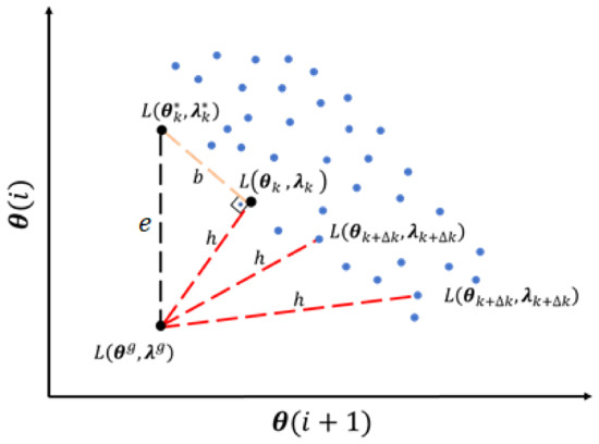
Figure 1.
The resulting space formed by the overall population originated by the algorithm. The relationship between the value of each particle with a theoretical global minimum is expressed in terms of Pythagorean theorem. Based on this theorem it is presented a schematical representation of the concepts used in the deductions of the Fisher–Snedecor test.
In Figure 1, represents the distance between the analytical optimum and the one optima found by the CSPSO , in other words it is the residual error of the objective function evaluation, is the projection of on a tangent plane to the , represents the difference between the analytical optimum and a given point in the CSPSO population . So, the error can be expressed by the triangle relationship in Figure 1 as:
The squared residual error, can be normalized in terms of variance of the complete population, , according to the following equation:
The error can be defined for all minima obtained in the optimization process, as follows:
The variance, , between each minimum found by the CSPSO and analytical optimum , is defined in Equation (5).
where is total number of iterations evaluated by the CSPSO. Therefore, it is possible to rewrite Equations (4) and (5) in the form of Equation (6).
As is the squared residual error of uncorrelated experiments (evaluations of the objective function), it follows a chi-squared distribution, . It is important to highlight that an experiment is referred here as a consult to the objective function. This consult should be an isolated event and a fact that is independent of the algorithm used to perform the optimization. This probability distribution has degrees of freedom, as follows:
Considering the same deduction, but now taking as reference the distance between the global analytical solution and the remaining points of the CSPSO population, represented in Figure 1 by . Then, , is defined by:
The variance, , between a minimum found by the CSPSO and a given point in the population, , is defined by:
Similar as done before with , Equations (8) and (9) can be transformed in:
Therefore, assuming also that becomes a chi-square distribution premise, whose degrees of freedom are expressed by , as follows:
where is the population size. Hence, the difference between the errors presented can be expressed by:
From the Pythagorean theorem is equal to . Furthermore, and are orthogonal to each other, as seen in Figure 1. Therefore, they are independent vectors; hence they are independent distributions. Knowing this, their ratio is equivalent to a Fisher-Snedecor distribution, as:
where is the confidence level of the Fisher–Snedecor test. Finally, the Taylor Series was expanded around the optimal point in terms of objective function as:
where is the gradient vector of the Lagragian and the Hessian matrix of the objective function, which is correlated to the covariance matrix of optimal points as [3,7]:
Replacing Equation (15) in Equation (14), it is possible to obtain:
Therefore, it is possible to rewrite Equation (13) through Equation (16), obtaining:
Assuming that is a good approximation for , the following test is obtained:
The deductions here presented culminated in the above Fisher-Snedecor test. That can be used to evaluate a population provided by a meta-heuristic method, the CSPSO in the present case, in terms of each local minima found. The population points that meet this criterion will compose the optimal region of the evaluated minima, building in this way a map of the multimodal landscape straightforward from the optimization results.
2.2. A Sliding Particle Swarm Optimization for Solving Constrained Optimization Problems
Particle swarm optimization is a meta-heuristic optimization technique based on the concept of a particle group of individuals that can hover over a determined optimization landscape, search region, in order to define the region topology. It was first presented by Kennedy and Eberhart (1995) as a method for the optimization of nonlinear functions that mimics the social behavior of living communities, for example, the birds’ flocks, which is nowadays the most common association to PSO. In the basic concept of this optimization strategy, each particle of the swarm has a specific position, , within the search area and a respective velocity, . This information is stored in an individual and a group memory, which are shared among all the members of the swarm in each iteration, . It can be represented as:
where and are the acceleration coefficients, and are random uniform generated numbers in a range between 0 and 1. Through Equations (19) and (20) the velocity and position of each particle after each iteration are computed. These values are based on the best position found among all the particles in all iterations, , and the particle own best position in the previous iterations, .
Several works have been published addressing this technique applied in different fields: parameters estimation [5,7], control system [9,10,11], and in optimization problems [12,13,14]. For the past two decades, studies have been published with developments and improvements in the PSO technique [12,15,16,17,18,19]
Ratnaweera et al. (2004), for example, proposed a self-organizing hierarchical particle swarm optimizer with time-varying acceleration coefficients (HPSO-TVAC). In the referred work, a PSO was developed to achieve fast convergence. This was done by introducing a necessary momentum for the particles through the elimination of the particle velocity term in Eq. 19 and introducing an adaptative acceleration coefficient. The authors showed through benchmark tests that their proposed HPSO was able to outperform previous strategy types of PSOs in most of the tests. When not outperforming, the HPSO presented similar results with faster convergence. In [18] another variant of PSO is presented, called parallel PSO. The algorithm was developed to deal with complex process optimization, that requires significant computational effort. The authors demonstrated the efficiency of the approach through the optimization of a chromatographic separation unit.
When the PSO is compared with other meta-heuristic methods it is considered to have simpler and easier implementation. Further comparisons are provided in the literature pointing out some advantages of the PSO strategy. For instance, in Kachitvichyanukul (2012) the genetic algorithms (GAs) are compared with PSO-based methods. The referred work evaluated the computational effort of both methods, and their respective precision, showing that the GAs present an exponential relation between the population size and the solution time, while the PSO presented a linear relationship. This gives margin to the employment of larger populations using PSO, which might be an advantage in complex optimizations. Furthermore, several works have been comparing the PSO with different GAs in different fields of application; most of these works point to a better performance of PSO [20,21,22].
A myriad of issues has been well addressed in the PSO literature, such as the acceleration coefficient, the particles inertia, initial velocity, etc. This last point, the initialization velocity, has been in analysis in the literature, e.g., Engelbrecht (2012) evaluated this issue concluding that the particles tend to leave the boundaries of the search space when the velocities are initiated randomly. The author demonstrated that the result is directly dependent on the method of initialization of the velocity of the particle, pointing out an initialization velocity equal to zero or random value around zero as the most adequate solution to avoid the roaming particles problem.
From one point of view, the literature about PSO is well developed. On the other hand, the application of PSO to solve multi-modal optimization problems is still an issue. This issue was addressed in Nogueira et al., (2020), where the authors proposed a PSO that can evaluate unconstrained multi-modal optimization problems. The PSO proposed in the referred work can cope with complex optimization systems. However, the standpoint of constrained problems still needs to be deepened.
Dealing with constrained objective functions and multilocal minima is a complex problem that can be found in several practical cases. In such a situation, the application of the usual PSO strategy might be limited due to the landscape nature, slight variation in the function peak height can generate significant changes in the position of the global optimum (Poli et al., 2007). Therefore, the flock might not have momentum enough to leave a local minimum, therefore getting stuck in it.
Thus, this work proposes a novel PSO modification, that can deal with the multi-minima problem in constrained optimization. We called this PSO version as constrained sliding particle swarm optimization (CSPSO). This was done by introducing a mutation on the individuals’ social learning, following a strategy like the one proposed by Nogueira et al. (2020).
This idea is presented in Figure 2 where it is found a given constrained function that has a total of five local minima. The mutable social component of the PSO will conduct the flock to hover the region R1 up to the region R3, inducing them to change their search area each time that a minimum is found. An ordinary PSO algorithm would find one of those minima and get stuck in that area. This is a problem in two ways: First, the results do not provide the full topography of the search region; second, in the drawing of the feasible operating region, because it is intended to evaluate all possible operating conditions that satisfy the process optimal conditions.
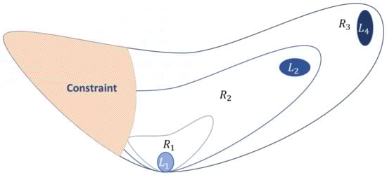
Figure 2.
Schematic representation of the possible search spaces (, and ) of a given function with and as local minima and and as constrained minima.
In this way, the CSPSO here proposed is based on the PSO-TVAC developed by Ratnaweera et al. (2004) and the SPSO developed by Nogueira et al., (2020), using the initial velocity equal to zero in order to achieve a better performance. The first step is then to set the acceleration coefficients, (, , , and ), the optimization constraints, the number of iterations , initial search region limits and set the maximum number of iterations as criterion to change the region.
Then the initialization procedure begins. The particles’ position is started within the first search regions, e.g., R1 in Figure 2. The initialization is done randomly generating, as:
where, is the inferior limit of the initial search region, is the superior limit, and is a random value between 0 and 1, introducing the randomness in the system.
After this, the initial velocities are set to zero and the maximum velocity, , can be calculated as:
Then the objective function and the set of constraints, , are evaluated for each particle position . There are two ways to address the constraints issue here, through a penalty function or straight evaluation. The first option introduces a new parameter to the optimization problem, which is the penalty. This parameter might affect the efficiency constraining the fly landscape. On the other hand, the straight evaluation of the constraints will make the algorithm computationally heavier. As the developed algorithm is meant to deal with complex optimization, it was decided to adopt both options which can be chosen by the user following the case study. This point is one of the points that this PSO variant diverges from the others found in the literature. Thus, the algorithm will work as presented in Figure 3, where δ is the constraint value, ∆ is the penalty factor.
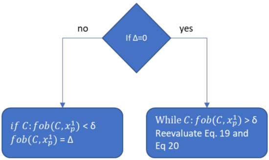
Figure 3.
Constraint evaluation diagram.
After the successful evaluation of the constraint, the acceleration coefficients ( and ) are computed as:
Then it is possible to evaluate the next iteration velocity, as:
where and are randomly generated variables. If the computed velocity is higher than , a new velocity value should be calculated using:
Then the new position can be computed, , as:
If the computed position does not respect the searching bounds or the internal restrictions, , then that position is set to the middle of the search area, .
At this point, the criteria for minimum local is evaluated based on the overall best optimal point, . If a value of optimal point is found to be equal or close to for several iterations, then a space restriction should be created. This constraint, created each time that a minimum is recognized, will serve as a social memory for the flock. Then, the gradual expansion of the search region of the CSPSO starts, when a minimum is recognized for the first time the flock should move from to , as in the example of Figure 2. Then gradually to and so on, after each new minimum is found, until the procedure is finished, and the total number of iterations is reached. Before each expansion of the search region, the information about the minimum point found will be stored in the social memory. If the algorithm does not find a new minimum, the region will expand until the global landscape is explored. At each expansion, the procedure here described is repeated. These last steps are the main differences between the proposed CSPSO and the others PSO variants found in the literature. Most of the other PSOs stop right before these steps. A pseudo-code of the proposed CSPSO is presented below Algorithm 1.
| Algorithm 1. A pseudo-code of the proposed CSPSO |
| Begin Set PSO parameters Acceleration coefficient 1:= Acceleration coefficient 2:= Define the value of the criteria χ for the maximum number of iteration within the same minima of a local minima l = 0 while (termination condition = false, expansion of search domain) to number of iterations to number of particles ) to number of dimensions update particle position and velocity ) to number of dimensions end |
3. Results
The CSPSO here proposed together with the likelihood analysis deduced was implemented in MATLAB. The results were compared with standard PSO strategies, and it was noted that, for all benchmarks, the ordinary PSO strategy was able to identify only one local minimum. Then, a series of benchmarks were used in order to evaluate the proposed methodology. This results section presents the performance of the methodology for five constrained benchmark problems. Three of them characterized by simple constraints, and two of them characterized by additional constraints in order to evaluate the robustness of the proposed methodology. In Table 1 is provided the CSPSO parameters used to solve this problem.

Table 1.
CSPSO parameters.
Benchmark 1-Ackley Function
The first benchmark is a continuous, multimodal, and non-convex function, defined on n-dimensional space. It is a well-known function for testing optimization algorithms. It is characterized by a large valley area with a slight inclination and several local small depressions; in its center is found a deep depression that configures the function global minimum. The function has one global minimum: at . The optimization problem that originates from Ackley function is written as:
where and are the constants and are usually equal to: , . The function area is usually constrained to a hypercube, in this case, defined by:
Table 1 provides the CSPSO parameters used to solve this problem.
As it is possible to see from Figure 4, the CSPSO provided a full picture of the Ackley Function topography. As it is possible to see from the 3D map this function has several local minima distributed along the way toward the global minima. The 2D map is then built using a projection of the 3D topography in a perpendicular plane. A contour map of this function was also added to the 2D map to provide a visual idea of where the minimum is located. Therefore, in the 2D map it is possible to see the contour lines, each line surrounding the minimum of that region. It is possible to see that the contour line forms small “puddles” around the local minima, where it is found the value corresponding to the objective function in that surrounding; furthermore, it is possible to see that these “puddles” are filled by the CSPSO confidence regions. Moving toward the center of Figure 4, the global minima is found, contour marked by the value 2, which is also well described by the confidence region. Thus, from the 2D map, it is possible to see that the methodology here proposed can identify all the local minima and the global minimum, while drawing their respective confidence regions. From the surface map, surface lines, it is possible to see that the confidence regions are precisely within the function minima and global minimum. The methodology was able to provide accurately the uncertainty map of each minimum found. Therefore, providing not only the optimal points but their corresponding uncertainty. Thus, the optimal inputs, and , are not an ordered pair but an ordered region within which it is possible to find several points that will lead to the same value of the objective function.
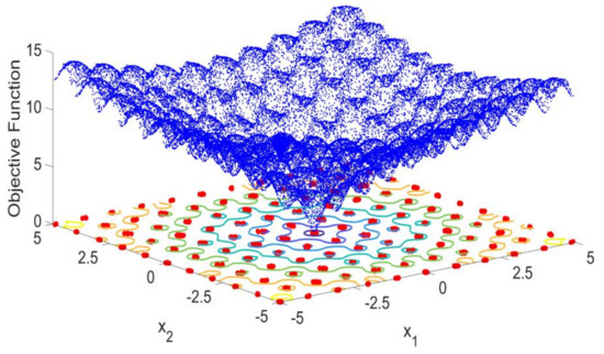
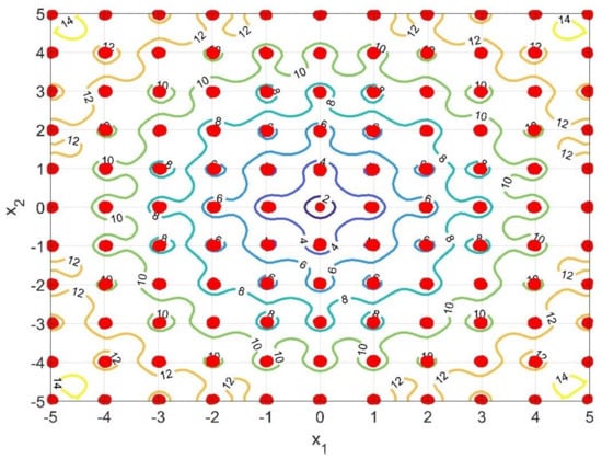
Figure 4.
Ackley Function 3D topography drawn by the proposed CSPSO and its corresponding 2D map of the local and global minima, with the confidence regions drawn by the deduced likelihood test. It is also presented a surface map of the objective function in order to show the location and values of the minima and global minimum.
Benchmark 2-Rastrigin Function
The Rastrigin Function is a continuous, non-convex function, defined on n-dimensional space. It is a representative example of a non-linear differentiable-multimodal function. This function is commonly used as a benchmark to test the performance of optimization algorithms due to its topography. In this case, there is no global minimum, but several local minima which in the present case are: is obtainable for , The optimization problem that originates from Rastrigin Function is written as:
s.t.
where is a constant and in the present case equal to 10, .
As it is possible to see from Figure 5 the CSPSO also provided a full picture of the Rastrigin Function topography. As it is possible to see from the 3D map this function has several local minima completely surrounded by maximum points. Therefore, this is a more complex landscape. The 2D map is then build using a projection of the 3D topography in a perpendicular plane. A contour map of this function was also added to the 2D map to provide a visual idea of where the minimum and maximum are located. In the 2D map, it is possible to see the contour lines, surrounding the minimum and maximum areas of the objective function landscape. Through the values in the contour lines, one can identify the maximum and minimum. Again, the contour line forms small “puddles” around the local minima and surrounding the maximum points. It is interesting to see that the proposed method was able to fill the “puddles” where the local minima are located, bypassing the maximum barriers. Moreover, from the 2D map, it is possible to see that the methodology proposed here can identify all the local minima, while drawing their respective confidence regions. The evidence provided by the first benchmark test is reinforced here by these new results. The methodology shows a significant efficiency to provide accurately the uncertainty map of each minimum found. From the surface map, it is possible to see that the confidence regions are precisely within the function minima.
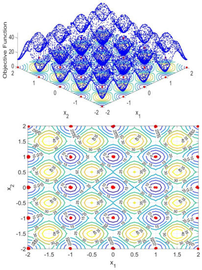
Figure 5.
Rastrigin Function 3D topography drawn by the proposed CSPSO and its corresponding 2D map of the local and global minima, with the confidence regions drawn by the deduced likelihood test. A surface map of the objective function is also presented in order to show the location and values of all minima.
Benchmark 3-Cross-in-Tray Function
The Cross-in-Tray Function is characterized as continuous, non-convex, multimodal, non-differentiable and defined on a 2-dimensional space. This function has a very peculiar shape in which a cross-like formation is found crossing the middle of its topography, forming four separate quarters. In each quarter of the function, several local minima are found. The optimization problem that originates from the Cross-in-Tray Function is written as:
s.t.
In this case, a shallow surface is presented that contains several minima. Therefore, it is a landscape more propone to hold the optimizer in one of the local minima. As before, the 2D map was built based on the projection of the 3D topography in a perpendicular plane. Through the contour lines, it is possible to see that there are slight differences between the minimum. Even though the proposed methodology was able to fill the minima found within the “puddles”. In this final test of this series of input constrained functions, the CSPSO also provided a full picture of the Cross-in-Tray Function topography, Figure 6. In the 2D map, it is possible to see that the proposed methodology can identify all the local minima even under peculiar topographies like this one. While drawing the local minima confidence regions, substantial evidence is provided that the methodology is efficient to accurately determine the uncertainty map of each minimum found. From the surface map it is possible to see that the confidence regions are precisely within the function minima.
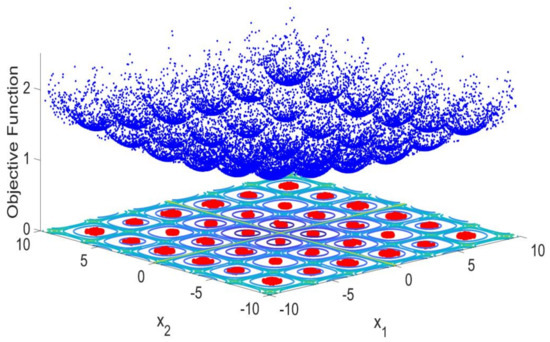
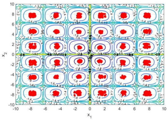
Figure 6.
Cross-in-Tray Function 3D topography drawn by the proposed CSPSO and its corresponding 2D map of the local and global minima, with the confidence regions drawn by the deduced likelihood test. A surface map of the objective function is also presented in order to show the location and values of the minima.
Benchmark 4-Egg Crate Function constrained
The Egg Crate Function is characterized to be continuous, not convex, multimodal, differentiable, separable, and defined on 2-dimensional space. In this case, an additional constraint was added to reduce the objective function area and evaluate the methodology robustness. The optimization problem that originates from Egg Crate Function with input and output constraints is written as:
s.t.
Figure 7 shows this new benchmark function in which were included constraints within the landscape. As it is possible to see from the 3D map, this function has a global minimum surrounded by maximum points and local minima. Therefore, this is a complex landscape, where it should be difficult to identify the global minima. The 3D map provides an overall idea of this landscape. A contour map of this function was also added to the 2D map providing a more detailed visualization of this topography in the 2D plane. Through the values in the contour lines, it is possible to see the maxima, minima, and global minimum. It is possible to see in this figure how the maxima contours are surrounding the global minimum, providing only a small access to this area. Furthermore, in this case, the proposed methodology was able to fully identify all the local minima and the global one. In this test it is possible to see that the CSPSO also provided a full picture of the constrained landscape. As it is possible to see in Figure 7, the introduced constraint removed four local minima from the landscape. In this case, it is observed that the CSPSO pointed in the constraint the direction of the local minima that are outside the constrained area. This is another evidence of the efficiency of the proposed methodology; this point can be seen in the 2D map. In this case, it is also demonstrated that it was possible to precisely draw the confidence regions of each local minimum.
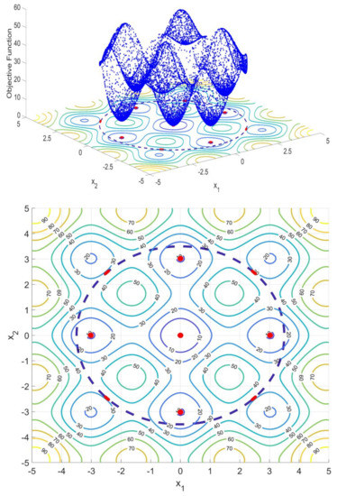
Figure 7.
Egg Crate Function with input and output constraints 3D topography drawn by the proposed CSPSO and its corresponding 2D map of the local and global minima, with the confidence regions drawn by the deduced likelihood test. A surface map of the objective function is also presented in order to show the location and values of the minima and global minimum.
Benchmark 5-Keane Function constrained
The Keane Function is defined as continuous, non-convex, multimodal, differentiable, non-separable and defined on a 2-dimensional space. As in the previous case, an additional constraint was added to reduce the objective function area and evaluate the methodology robustness. The optimization problem that originates Keane Function is written as:
s.t.
Figure 8 shows this new benchmark function in which were included constraints within the landscape. In this test, it is possible to see that the CSPSO also provided a full picture of the constrained landscape. As it is possible to see in Figure 8 the introduced constraint removed seven local minima from the landscape. In this case, there were two minima beyond the constraint, but close to it. However, the CSPSO could not point the existence of these minima beyond the constraint. Probably this is due to the landscape of the Keane Function constrained, which has a deep depression close to the restriction. This depression might work as a gravitational pole that attracts all the particles close by. On the other hand, the CSPSO was able to effectively identify all minima within the constrained landscape, proving the efficiency of the proposed method.
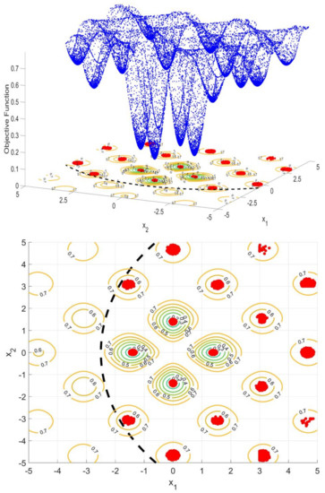
Figure 8.
Keane Function constrained with input and output constraints 3D topography drawn by the proposed CSPSO and its corresponding 2D map of the local and global minima, with the confidence regions drawn by the deduced likelihood test. A surface map of the objective function is also presented in order to show the location and values of the minima and global minimum.
Benchmark 5–Himmelblau Function
The Himmelblau Function is defined as a continuous, non-convex, multimodal, differentiable and defined on 2-dimensional space. This function is characterized by a flat landscape, which makes the search for the minimum more difficult. The optimization problem that originates Himmelblau Function is written as:
Figure 9 shows this final benchmark which has different properties than the previous ones. As it is possible to see this function has a very flat landscape where it is possible to find four local minima: ; ; ; . The contour map is also provided for this function providing a more detailed visualization of this topography in 2D plane. It is possible to see that in this case, the above mentioned “puddles” are not found in the contours. Instead, two large areas for objective function equal to 100 are observed. Within these areas, the local minima are found. This is a representation of how flat/shallow the landscape is, which barely changes its slop until the minima are found. Moreover, in this case, the proposed methodology was able to fully identify all the local minima and the global ones.
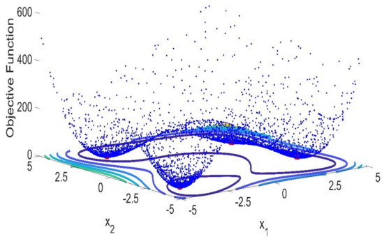
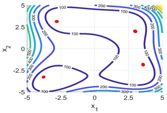
Figure 9.
Himmelblau Function 3D topography drawn by the proposed CSPSO and its corresponding 2D map of the local and global minima, with the confidence regions drawn by the deduced likelihood test. A surface map of the objective function is also presented in order to show the location and values of the minima and global minimum.
A case study–Optimization of a True Moving Bed Reactor
True moving bed reactor (TMBR) is a multifunctional unit that is capable of integrating reaction and separation simultaneously, being an alternative to the traditional way of production where it is found one specific unit for each step (reaction and separation) of the production route. It is highlighted as an efficient way to leverage the potential of systems in which the reactions are limited by equilibrium [23,24,25,26]. The equilibrium conversion is not a limitation in those units because one or more of the products are continuously removed from the reaction zone [27]. However, this system presents complex dynamics and system nonlinearity which make the unit optimization and control very difficult tasks.
In [28] a true moving bed reactor was proposed and optimized to perform the synthesis of n-propyl propionate. Please refer to this work if the reader is interested in more details about the process, phenomenological model, and the system. The optimization problem for the synthesis of n-propyl propionate in a TMBR unit is a 5-dimensional problem and was written in [28] as:
s.t.
where , is the extract stream purity, , is the raffinate stream purity, EC, is the eluent consumption, and is the unit productivity, is the minimum requirement for the purities. As it is an input/output system, the processes output are dependent on the process input, which are here the decision variables,, in this case operating flow rates of the process: feed flow rate (), eluent flow rate (, recycling flow rate), extract flow rate (), and solid flow rate . Therefore, the goal is to maximize the productivity while minimizing the eluent consumption and keeping the purities as close as possible to its target. This objective function has two local minima.
Figure 10 presents the results obtained after applying the proposed methodology to solve the TMBR optimization problem. It is provided in the figure the objective function landscape, the optimal points confidence regions, and the contour of the expected region for the local minima. The information about the contour of the expected region was obtained from [29] and used as a reference to check the CSPSO result. As it is possible to see from Figure 9, the algorithm was able to identify the two local minima of the objective function and describe with precision the confidence region of the optimal point, with a confidence level of 99%. This means that any of these points inside the confidence region will generate an optimal operating condition in the process.
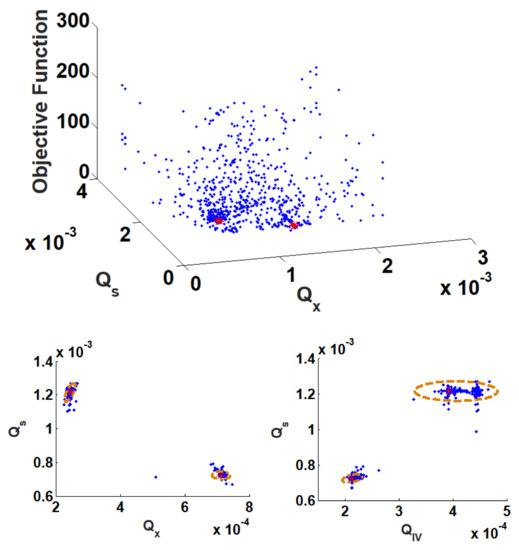
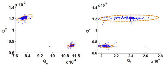
Figure 10.
Process optimization results based on the proposed methodology. At the top of the figure is presented the objective function landscape, then it is presented the operating confidence region defined by the proposed test and the contour area where the local minima are located.
4. Conclusions
This work presented the mathematical deductions of a likelihood test to evaluate confidence regions of optimal points provided by population-based methods. A novel particle swarm optimization algorithm was proposed to apply the proposed likelihood test in the identification of multi-local minima and concomitantly map their correlated uncertainties for constrained optimizations. The proposed optimization algorithm is here called constrained sliding particle swarm optimization (CSPSO).
A series of benchmark tests were done in order to evaluate the efficiency, consistency, and robustness of the proposed methodology. Six optimization problems of multi-modal functions were tested. The CSPSO was able to identify all local-minima and global minimum, when existent, for all the benchmarks here tested. Furthermore, through the population and using the proposed likelihood test, it was possible to draw the confidence regions of each local-minima and the global one when existent. A final test involving the optimization of a chemical unit, a true moving bed reactor, was then provided. In this last optimization case, it was possible to demonstrate the application of the proposed methodology in a practical problem. The method was able to identify all the local minima of this last optimization problem. Furthermore, as the methodology was able to identify with precision the optimal regions, it proves that the distribution of errors, and , are distribution, thus in accordance with the proposed methodology.
Therefore, it was possible to map the uncertainties of the optimal points, extending the result of the optimization algorithm from a defined value to a feasible region. All the decision variables mapped within the optimal regions lead to an optimal value of the objective function satisfying the problem constraints.
Author Contributions
Conceptualization, I.B.R.N., M.A.F.M.; methodology, I.B.R.N., C.M.R.; writing—original draft preparation, I.B.R.N., C.M.R.; writing—review and editing, I.B.R.N., M.A.F.M. and A.M.R.; supervision, I.B.R.N., J.M.L., A.E.R., A.M.R., M.A.F.M. All authors have read and agreed to the published version of the manuscript.
Funding
This work was financially supported by: Project—NORTE-01-0145-FEDER-029384 funded by FEDER funds through NORTE 2020-Programa Operacional Regional do NORTE—and by national funds (PIDDAC) through FCT/MCTES. This work was also financially supported by: Base Funding—UIDB/50020/2020 of the Associate Laboratory LSRE-LCM—funded by national funds through FCT/MCTES (PIDDAC), Capes for its financial support, financial code 001 and FCT-Fundação para a Ciência e Tecnologia under CEEC Institucional program.
Acknowledgments
This work was financially supported by: Project-NORTE-01-0145-FEDER-029384 funded by FEDER funds through NORTE 2020-Programa Operacional Regional do NORTE–and by national funds (PIDDAC) through FCT/MCTES. This work was also financially supported by: Base Funding-UIDB/50020/2020 of the Associate Laboratory LSRE-LCM-funded by national funds through FCT/MCTES (PIDDAC), Capes for its financial support, financial code 001 and FCT–Fundação para a Ciência e Tecnologia under CEEC Institucional program.
Conflicts of Interest
The authors declare no conflict of interest.
References
- Park, C. Determination of the joint confidence region of the optimal operating conditions in robust design by the bootstrap technique. Int. J. Prod. Res. 2013, 51, 4695–4703. [Google Scholar] [CrossRef] [Green Version]
- Nogueira, I.B.R.; Martins, M.A.F.; Requião, R.; Oliveira, A.R.; Viena, V.; Koivisto, H.; Rodrigues, A.E.; Loureiro, J.M.; Ribeiro, A.M. Optimization of a True Moving Bed unit and determination of its feasible operating region using a novel Sliding Particle Swarm Optimization. Comput. Ind. Eng. 2019, 135. [Google Scholar] [CrossRef]
- Schwaab, M.; Biscaia, E.C.; Monteiro, J.L.; Pinto, J.C. Nonlinear parameter estimation through particle swarm optimization. Chem. Eng. Sci. 2008, 63, 1542–1552. [Google Scholar] [CrossRef]
- Benyahia, B.; Latifi, M.A.; Fonteix, C.; Pla, F. Emulsion copolymerization of styrene and butyl acrylate in the presence of a chain transfer agent. Part 2: Parameters estimability and confidence regions. Chem. Eng. Sci. 2013, 90, 110–118. [Google Scholar] [CrossRef] [Green Version]
- Nogueira, I.B.R.; Faria, R.P.V.; Rodrigues, A.E.; Loureiro, J.M.; Ribeiro, A.M. Chromatographic studies of n-Propyl Propionate, Part II: Synthesis in a fixed bed adsorptive reactor, modelling and uncertainties determination. Comput. Chem. Eng. 2019, 128, 164–173. [Google Scholar] [CrossRef]
- Nogueira, I.B.R.; Faria, R.P.V.; Requião, R.; Koivisto, H.; Martins, M.A.F.; Rodrigues, A.E.; Loureiro, J.M.; Ribeiro, A.M. Chromatographic studies of n-Propyl Propionate: Adsorption equilibrium, modelling and uncertainties determination. Comput. Chem. Eng. 2018, 119, 371–382. [Google Scholar] [CrossRef]
- Bard, Y. Nonlinear Parameter Estimation; Academic Press: New York, NY, USA, 1975. [Google Scholar]
- Kennedy, J.; Eberhart, R. Particle swarm optimization. In Proceedings of the ICNN’95-International Conference on Neural Networks, Perth, Australia, 27 November–1 December 1995; Volume 4, pp. 1942–1948. [Google Scholar]
- Al-Dunainawi, Y.; Abbod, M.F.; Jizany, A. A new MIMO ANFIS-PSO based NARMA-L2 controller for nonlinear dynamic systems. Eng. Appl. Artif. Intell. 2017, 62, 265–275. [Google Scholar] [CrossRef] [Green Version]
- Nery, G.A.; Martins, M.A.F.; Kalid, R. A PSO-based optimal tuning strategy for constrained multivariable predictive controllers with model uncertainty. ISA Trans. 2014, 53, 560–567. [Google Scholar] [CrossRef]
- Soufi, Y.; Bechouat, M.; Kahla, S. Fuzzy-PSO controller design for maximum power point tracking in photovoltaic system. Int. J. Hydrogen Energy 2017, 42, 8680–8688. [Google Scholar] [CrossRef]
- Jiang, Y.; Hu, T.; Huang, C.; Wu, X. An improved particle swarm optimization algorithm. Appl. Math. Comput. 2007, 193, 231–239. [Google Scholar] [CrossRef]
- Parsopoulos, K.E.; Vrahatis, M.N. Particle swarm optimization method in multiobjective problems. In Proceedings of the 2002 ACM symposium on Applied computing, Spain, Madrid, 11–14 March 2002; pp. 603–607. [Google Scholar]
- Nogueira, I.B.R.; Martins, M.A.F.; Regufe, M.J.; Rodrigues, A.E.; Loureiro, J.M.; Ribeiro, A.M. Big Data-Based Optimization of a Pressure Swing Adsorption Unit for Syngas Purification: On Mapping Uncertainties from a Metaheuristic Technique. Ind. Eng. Chem. Res. 2020. [Google Scholar] [CrossRef]
- Ratnaweera, A.; Halgamuge, S.K.; Watson, H.C. Self-organizing hierarchical particle swarm optimizer with time-varying acceleration coefficients. IEEE Trans. Evol. Comput. 2004, 8, 240–255. [Google Scholar] [CrossRef]
- Engelbrecht, A. Particle swarm optimization: Velocity initialization. In Proceedings of the 2012 IEEE Congress on Evolutionary Computation, Brisbane, Australia, 10–15 June 2012; pp. 10–15. [Google Scholar] [CrossRef] [Green Version]
- Liu, P.; Liu, J. Multi-leader PSO (MLPSO): A new PSO variant for solving global optimization problems. Appl. Soft Comput. J. 2017, 61, 256–263. [Google Scholar] [CrossRef]
- Matos, J.; Faria, R.P.V.; Nogueira, I.B.R.; Loureiro, J.M.; Ribeiro, A.M. Optimization strategies for chiral separation by true moving bed chromatography using Particles Swarm Optimization (PSO) and new Parallel PSO variant. Comput. Chem. Eng. 2019, 123, 344–356. [Google Scholar] [CrossRef]
- Kachitvichyanukul, V. Comparison of Three Evolutionary Algorithms: GA, PSO, and DE. Ind. Eng. Manag. Syst. 2012, 11, 215–223. [Google Scholar] [CrossRef] [Green Version]
- Hassan, R.; Cohanim, B.; Weck, O. de A comparison of particle swarm optimization and the genetic algorithm. In Proceedings of the 46th AIAA/ASME/ASCE/AHS/ASC Structures, Structural Dynamics and Materials Conference, Austin, TX, USA, 18–21 April 2005; pp. 1–13. [Google Scholar] [CrossRef]
- Duan, Y.; Harley, R.G.; Habetler, T.G. Comparison of Particle Swarm Optimization and Genetic Algorithm in the design of permanent magnet motors. In Proceedings of the 2009 IEEE 6th International Power Electronics and Motion Control Conference, Wuhan, China, 17–20 May 2009; pp. 822–825. [Google Scholar]
- Panda, S.; Padhy, N.P. Comparison of particle swarm optimization and genetic algorithm for FACTS-based controller design. Appl. Soft Comput. J. 2008, 8, 1418–1427. [Google Scholar] [CrossRef]
- Minceva, M.; Rodrigues, A.E. Simulated moving-bed reactor: Reactive-separation regions. AIChE J. 2005, 51, 2737–2751. [Google Scholar] [CrossRef]
- Gonçalves, J.C.; Rodrigues, A.E. Simulated moving bed reactor for p-xylene production: Dual-bed column. Chem. Eng. Process. Process. Intensif. 2016, 104, 75–83. [Google Scholar] [CrossRef]
- Pereira, C.S.M.; Gomes, P.S.; Gandi, G.K.; Silva, V.M.T.M.; Rodrigues, A.E. Multifunctional Reactor for the Synthesis of Dimethylacetal. Ind. Eng. Chem. Res. 2008, 47, 3515–3524. [Google Scholar] [CrossRef]
- Pereira, C.S.M.; Rodrigues, A.E. Process intensification: New technologies (SMBR and PermSMBR) for the synthesis of acetals. Catal. Today 2013, 218–219, 148–152. [Google Scholar] [CrossRef]
- Constantino, D.S.M.; Pereira, C.S.M.; Faria, R.P.V.; Ferreira, A.F.P.; Loureiro, J.M.; Rodrigues, A.E. Synthesis of butyl acrylate in a fixed-bed adsorptive reactor over Amberlyst 15. AIChE J. 2015, 61, 1263–1274. [Google Scholar] [CrossRef]
- Nogueira, I.B.R.; Viena, V.; Rodrigues, A.E.; Loureiro, J.M.; Ribeiro, A.M. Dynamics of a True Moving Bed Reactor: Synthesis of n-Propyl Propionate and an alternative optimization method. Chem. Eng. Process. Process. Intensif. 2020, 148, 107821. [Google Scholar] [CrossRef]
- Nogueira, I.B.R. Optimization and Control of TMB, SMB and SMBR Units; University of Porto: Porto, Portugal, 2018. [Google Scholar]
Publisher’s Note: MDPI stays neutral with regard to jurisdictional claims in published maps and institutional affiliations. |
© 2021 by the authors. Licensee MDPI, Basel, Switzerland. This article is an open access article distributed under the terms and conditions of the Creative Commons Attribution (CC BY) license (https://creativecommons.org/licenses/by/4.0/).