Multi-Transformer: A New Neural Network-Based Architecture for Forecasting S&P Volatility

Abstract

Events such as the Financial Crisis of 2007–2008 or the COVID-19 pandemic caused significant losses to banks and insurance entities. They also demonstrated the importance of using accurate equity risk models and having a risk management function able to implement effective hedging strategies. Stock volatility forecasts play a key role in the estimation of equity risk and, thus, in the management actions carried out by financial institutions. Therefore, this paper has the aim of proposing more accurate stock volatility models based on novel machine and deep learning techniques. This paper introduces a neural network-based architecture, called Multi-Transformer. Multi-Transformer is a variant of Transformer models, which have already been successfully applied in the field of natural language processing. Indeed, this paper also adapts traditional Transformer layers in order to be used in volatility forecasting models. The empirical results obtained in this paper suggest that the hybrid models based on Multi-Transformer and Transformer layers are more accurate and, hence, they lead to more appropriate risk measures than other autoregressive algorithms or hybrid models based on feed forward layers or long short term memory cells.

1. Introduction

Since the Financial Crisis of 2007–2008, financial institutions have enhanced their risk management framework in order to meet the new regulatory requirements set by Solvency II or Basel III. These regulations have the aim of measuring the risk profile of financial institutions and minimizing losses from unexpected events such as the European sovereign debt crisis or COVID-19 pandemic. Even though banks and insurance entities have reduced their losses thanks to the efforts made in the last years, unexpected events still cause remarkable losses to financial institutions. Thus, efforts are still required to further enhance market and equity risk models in which stock volatility forecasts play a fundamental role. Volatility, understood as a measure of an asset uncertainty [1,2], is not directly observed in stock markets. Thus, taking into consideration the stock market movements, a statistical model is applied in order to compute the volatility of a security.

GARCH-based models [3,4] are widely used for volatility forecasting purposes. This family of models is especially relevant because it takes into consideration the volatility clustering observed by [5]. Nevertheless, as the persistence of conditional variance tends to be close to zero, Refs. [6,7,8,9] developed more flexible variations of the traditional GARCH models. In addition, the models introduced by [10] (EGARCH) and [11] (GJR-GARCH) take into consideration that stocks volatility behaves differently depending on the market trend, bearish or bullish. Multivariate GARCH models were developed by [12,13]. Bollerslev et al. [14] applied the previous model to financial time series, while [15] introduced a time-varying multivariate GARCH. Dynamic conditional correlation GARCH, BEKK-GARCH and Factor-GARCH were other variants of this family that were developed by [16,17,18], respectively. Finally, it is worth mentioning that, in contrast to classical GARCH, the first-order zero-drift GARCH model (ZD-GARCH) proposed by [19] is non-stationary regardless of the sign of Lyapunov exponent and, thus, it can be used for studying heteroscedasticity and conditional heteroscedasticity together.

Another relevant family is composed by stochastic volatility models. As they assume that volatility follows its own stochastic process, these models are widely used in combination with Black–Scholes formula to assess derivatives price. The most popular process of this family is the [20] model which assumes that volatility follows an Cox-Ingersoll-Ross [21] process and stock returns a Brownian motion. The main challenge of the Heston model is the estimation of its parameters. Refs. [22,23] proposed a generalized method of moments to obtain the parameters of the stochastic process, while [24,25,26,27] used a simulation approach to estimate them. Other relevant stochastic volatility processes are Hull–White [28] and SABR [29] models.

The last relevant family is composed of those models based on machine and deep learning techniques. Even though GARCH models are considered part of the machine learning tool-kit, these models are considered another different family due to the significant importance that they have in the field of stock volatility. Thus, this family takes into consideration the models based on the rest of the machine and deep learning algorithms such as artificial neural networks [30], gradient boosting with regression trees [31], random forests [32] or support vector machines [33]. Refs. [34,35,36] applied machine learning techniques such as Support Vector Machines or hidded Markov models to forecast financial time series. Hamid and Iqbid [37] applied Artificial Neural Networks (ANNs) to demonstrate that the implied volatility forecasted by this algorithm is more accurate than Barone–Adesi and Whaley models.

ANNs have been also combined with other statistical models with the aim of improving the forecasting power of individual ANNs. The most common approach applied in the field of stocks volatility is merging GARCH-based models with ANNs. Refs. [38,39,40,41,42,43,44] developed different architectures based in the previous approach for stock volatility forecasting purposes. All these authors demonstrated that hybrid models overcome the performance of traditional GARCH models in the field of stock volatility forecasting. It is also worth mentioning the contribution of [45], who combined different GARCH models with ANNs in order to compare their predictive power. ANN-GARCH models have been also applied to forecast other financial time series such as metals [46,47] or oil [48,49] volatility. Apart from the combination with GARCH-based models, ANNs have been merged with other models for volatility forecasting purposes. Ramos-Pérez et al. [50] merged ANNs, random forests, support vector machines (SVM) and gradient boosting with regression trees in order to forecast S&P500 volatility. This model overcame the performance of a hybrid model based on feed forward layers and GARCH. Vidal and Kristjanpoller [51] proposed an architecture based on convolutional neural networks (CNNs) and long-short term memory (LSTM) units to forecast gold volatility. LSTMs were also used by [52] to forecast currency exchange rates volatility. It is also worth mentioning that GARCH models have not been only merged with ANNs, Peng et al. [53] combined SVM with GARCH-based models in order to predict cryptocurrencies volatility.

The aim of this paper is to introduce a more accurate stock volatility model based on an innovative machine and deep learning technique. For this purpose, hybrid models based on merging Transformer and Multi-Transformer layers with other approaches such as GARCH-based algorithms or LSTM units are introduced by this paper. Multi-Transformer layers, which are also introduced in this paper, are based on the Transformer architecture developed by [54]. Transformer layers have been successfully implemented in the field of natural language processing (NLP). Indeed, the models developed by [55,56] demonstrated that Transformer layers are able to overcome the performance of traditional NLP models. Thus, this recently developed architecture is currently considered the state-of-the-art in the field of NLP. In contrast to LSTM, Transformer layers do not incorporate recurrence in their structure. This novel structure relies on a multi-head attention mechanism and positional embeddings in order to forecast time series. As [54] developed Transformer for NLP purposes, positional embeddings are used in combination with word embeddings. The problem faced in this paper is the forecasting of stock volatility and, thus, the word embedding is not needed and the positional embedding has been modified as it is explained in Section 2.4.

In contrast to Transformer, Multi-Transformer randomly selects different subsets of training data and merges several multi-head attention mechanisms to produce the final output. Following the intuition of bagging, the aim of this architecture is to improve the stability and accurateness of the attention mechanism. It is worth mentioning that the GARCH-based algorithms used in combination with Transformer and Multi-Transformer layers are GARCH, EGARCH, GJR-GARCH, TrGARCH, FIGARCH and AVGARCH.

Therefore, three main contributions are provided by this study. First, Transformer layers are adapted in order to forecast stocks volatility. In addition, an extension of the previous structure is presented (Multi-Transformer). Second, this paper demonstrates that merging Transformer and Multi-Transformer layers with other models lead to more accurate volatility forecasting models. Third, the proposed stock volatility models generate appropriate risk measures in low and high volatility regimes. The Python implementation of the volatility models proposed in this paper is available in this repository.

As it is shown by the extensive literature included in this section, stock volatility forecasting has been a relevant topic not only for financial institutions and regulators but also for the academia. As financial markets can suffer drastic sudden drops, it is highly desirable to use models that can adequately forecast volatility. It is also useful to have indicators that can accurately measure risk.This paper makes use of recent deep and machine learning techniques to create more accurate stock volatility models and appropriate equity risk measures.

The rest of the paper is organized as follows: Section 2 describes the dataset, the measures used for validating the volatility forecasts and provides a look at the volatility models used as benchmark. Then, this section presents the volatility forecasting models proposed in this paper, which are based on Transformer and Multi-Transformer layers. As NLP Transformers need to be adapted in order to be used for volatility forecasting purposes and Multi-Transformer layers are introduced by this paper, explanations about the theoretical background of these structures are also given. The analysis of empirical results is presented in Section 3. Finally, the results are discussed in Section 4, followed by concluding remarks in Section 5.

2. Materials and Methods

This section is divided in five different subsections. The first one (Section 2.1) describes the data for fitting the models. The measures for validating the accuracy and value at risk (VaR) of each stock volatility model are explained in Section 2.2. Section 2.3 presents the stock volatility models and algorithms used for benchmarking purposes. Section 2.4 explains the adaptation of Transformer layers in order to be used for volatility forecasting purposes and, finally, the Multi-Transformer layers and the models based on them are presented in Section 2.5.

2.1. Data and Model Inputs

The proposed architectures and benchmark models are fitted using the rolling window approach (see Figure 1). This widely used methodology has been applied in finance, among others, by [57,58,59,60]. Rolling window uses a fixed sample length for fitting the model and, then, the following step is forecasted. As in this paper the window size is set to 650 and the forecast horizon to 1, the proposed and benchmark models are fitted using the last 650 S&P trading days and, then, the next day volatility is forecasted. This process is repeated until the whole period under analysis is forecasted. The periods used as training and testing set will be defined at the end of this subsection.

The input variables of the models proposed are the daily logarithmic returns ($r_{t-i}$) and the standard deviation of the last five daily logarithmic returns:

$$\begin{array}{c}\hfill {\sigma }_{t-1}=\sqrt{\frac{{\sum }_{i=1}^n(r_{t-i}-E\left[r\right]{)}^2}{n-1}}\end{array}$$

(1)

As Multi-Transformer, Transformer and LSTM layers are able to manage time series, a lag of the last 10 observations of the previous variables are taken into consideration for fitting these layers. Thus, the input variables are:

$$\begin{array}{c}\hfill X_1=({\sigma }_{t-1},{\sigma }_{t-2},\cdots ,{\sigma }_{t-10})\end{array}$$

(2)

$$\begin{array}{c}\hfill X_2=(r_{t-1},r_{t-2},\cdots ,r_{t-10})\end{array}$$

(3)

In accordance with other studies such as [38] or [50], the realized volatility is used as response variable for the models based on ANNs;

$$\begin{array}{c}\hfill Y={\widehat{\sigma }}_{i,t}=\sqrt{\frac{{\sum }_{n=0}^{i-1}(r_{t+n}-E\left[r_f\right]{)}^2}{i-1}}\end{array}$$

(4)

where $E\left[r_f\right]={\sum }_{n=0}^{i-1}{r}_{t+n}/i$ and $i=5$. As shown in the previous formula, the realized volatility can be defined as the standard deviation of future logarithmic returns.

The dataset for fitting and evaluating the volatility forecasting models contains market data of S&P from 1 January 2008 to 31 December 2020. The optimum configuration of the models is obtained by applying the rolling window approach and selecting the configuration which minimizes the error (RMSE) in the period going from 1 January 2008 to 31 December 2015. The optimum configuration in combination with the rolling window methodology is applied in order to forecast the volatility contained in the testing set (from 1 January 2016 to 31 December 2020). The empirical results presented in Section 3.2 are based on the forecasts of the testing set.

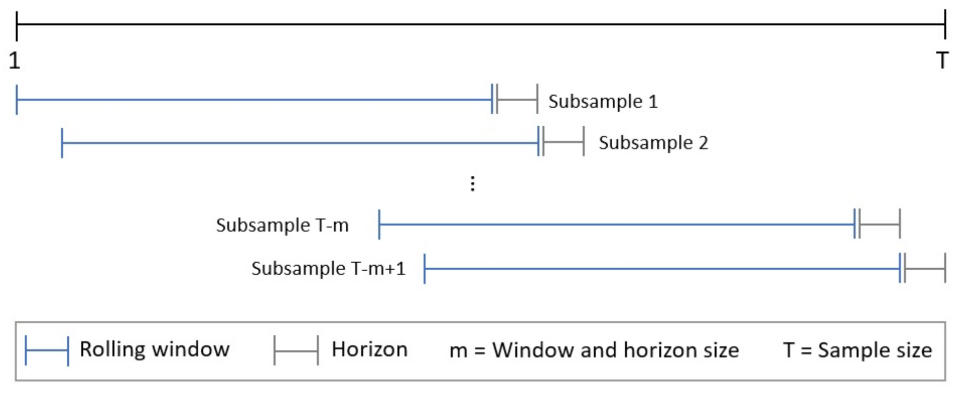
2.2. Models Validation

This subsection presents the measures selected for validating and comparing the performance of the benchmark models with the algorithms proposed in this paper.

The mean absolute value ($MAE$) and the root mean squared error ($RMSE$) have been selected for validating the forecasting power of the different stock volatility models:

$$MAE=\sum _{t=1}^N\frac{\mid {\sigma }_{i,t}-{\widehat{\sigma }}_{i,t}\mid }{N}/RMSE=\sum _{t=1}^N\frac{{({\sigma }_{i,t}-{\widehat{\sigma }}_{i,t})}^2}{N}$$

(5)

where N is the total number of observations.

The validation carried out by this study is not only interested on the accuracy, but also on the appropriateness of the risk measures generated by the different stock volatility forecasting models. In accordance with Solvency II Directive, $99.5\%$ VaR has been selected as risk measure. Although Solvency II has the aim of obtaining the yearly VaR, the calculations carried out in this paper will be based on a daily VaR in order to have more data points and, thus, more robust conclusions on the performance of the different models. The parametric approach developed by [61] is used for validating the different VaR estimations. The aim of this test is accepting (or rejecting) the hypothesis that the number of VaR exceedances are aligned with the confidence level selected for calculating the risk measure. In addition to the previous test, the approach suggested by [62] is also applied in order to validate the appropriateness of VaR.

2.3. Benchmark Models

This subsection introduces the benchmark models used in this paper: GARCH, EGARCH, AVGARCH, GJR-GARCH, TrARCH, FIGARCH and two architectures that combine GARCH-based algorithms with ANN and LSTM, respectively. The GARCH-based algorithms will be fitted assuming that innovations, ${ϵ}_t$, follow a Student’s t-distribution. Thus, the returns generated by these models follow a conditional t-distribution [63].

The generalized autoregressive conditional heteroskedasticity (GARCH) model developed by [4] has been widely used for stock volatility forecasting purposes. GARCH(p,q) has the following expression:

$${\widehat{\sigma }}_t^2=\omega +\sum _{i=1}^q{\alpha }_i{r}_{t-i}^2+\sum _{i=1}^p{\beta }_i{\sigma }_{t-i}^2/{\widehat{r}}_t={\widehat{\sigma }}_t{ϵ}_t$$

(6)

where ${\omega }_i$, ${\alpha }_i$ and ${\beta }_i$ are the parameters to be estimated, $r_{t-i}$ the previous returns and ${\sigma }_{t-i}^2$ the last observed volatility. As previously stated, innovations (${ϵ}_t$) follow a Student’s t-distribution.

The absolute value GARCH [64], AVGARCH(p,q), is similar to the traditional GARCH model. In this case, the absolute value of previous return and volatility is taken into consideration to forecast volatility:

$$\begin{array}{c}\hfill {\widehat{\sigma }}_t=\omega +\sum _{i=1}^q{\alpha }_i\mid r_{t-i}\mid +\sum _{i=1}^p{\beta }_i{\sigma }_{t-i}\end{array}$$

(7)

As volatility behaves differently depending on the market tendency, models such as EGARCH, GJR-GARCH or TrGARCH were developed. EGARCH(p,q) [10] has the following expression for the logarithm of stocks volatility:

$$\begin{array}{cc}\hfill & log{\widehat{\sigma }}_t^2=\omega +\sum _{i=1}^p{\alpha }_{i}log{\widehat{\sigma }}_{t-i}^2+\sum _{i=1}^q({\beta }_i{e}_{t-i}+{\gamma }_i(\mid e_{t-i}\mid -E(\mid e_{t-i}\mid )))\hfill \end{array}$$

(8)

where ${\omega }_i$, ${\alpha }_i$, ${\beta }_i$ and ${\gamma }_i$ are the parameters to be estimated and $e_t=r_t/{\sigma }_t$. The GJR-GARCH(p,o,q) developed by [11] has the following expression:

$$\begin{array}{c}\hfill {\widehat{\sigma }}_t^2=\omega +\sum _{i=1}^q{\alpha }_i{r}_{t-i}^2+\sum _{i=1}^o{\gamma }_i{r}_{t-i}^2{I}_{[r_{t-1}<0]}+\sum _{i=1}^p{\beta }_i{\sigma }_{t-i}^2\end{array}$$

(9)

As with EGARCH model, ${\omega }_i$, ${\alpha }_i$, ${\beta }_i$ and ${\gamma }_i$ are the parameters to be estimated. $I_{[r_{t-1}<0]}$ takes the value of 1 when the subscript condition is met. Otherwise $I_{[r_{t-1}<0]}=0$. The volatility of the Threshold GARCH(p,o,q) (TrGARCH) model is obtained as follows:

$$\begin{array}{c}\hfill {\widehat{\sigma }}_t=\omega +\sum _{i=1}^q{\alpha }_i\mid r_{t-i}\mid +\sum _{i=1}^o{\gamma }_i\mid r_{t-i}\mid I_{[r_{t-i}<0]}+\sum _{i=1}^p{\beta }_i{\sigma }_{t-i}\end{array}$$

(10)

As with the previous two architectures, ${\omega }_i$, ${\alpha }_i$, ${\beta }_i$ and ${\gamma }_i$ are the model parameters. The last GARCH-based algorithm used in this paper is the fractionally integrated GARCH (FIGARCH) model developed by [65]. The conditional variance dynamic is

$$\begin{array}{c}\hfill {\widehat{\sigma }}_t=\omega +\left[1-\beta L-\varphi L{(1-L)}^d\right]{ϵ}_t^2+\sigma h_{t-1}\end{array}$$

(11)

where L is the lag operator and d the fractional differencing parameter.

In addition to the previous approaches, two other hybrid models based on merging autoregressive algorithms with ANNs and LSTMs are also used as benchmark. Figure 2 shows the architecture of ANN-GARCH and LSTM-GARCH. The inputs of the algorithms are the following:

• The last daily logarithmic return, $r_{t-1}$, for the ANN-GARCH and the last ten in the case of the LSTM-GARCH (as explained in Section 2.1).
• The standard deviation of the last five daily logarithmic returns:

  $$\begin{array}{c}\hfill {\sigma }_{t-1}=\sqrt{\frac{{\sum }_{i=1}^n(r_{t-i}-E\left[r\right]{)}^2}{n-1}}\end{array}$$

  (12)

  where $E\left[r\right]={\sum }_{i=1}^n{r}_{t-i}/n$ and $n=5$. As with the previous input variable, the last standard deviation is considered in the ANN-GARCH, whereas the last ten are taken into consideration by the LSTM-GARCH architecture.

The GARCH-based algorithms included within the ANN-GARCH and LSTM-GARCH models are the six algorithms previously presented in this same subsection (GARCH, EGARCH, AVGARCH, GJR-GARCH, TrARCH, FIGARCH).

As explained in Section 2.1, the true implied volatility, ${\sigma }_{i,t}$, is used as response variable to train the models. This variable is the standard deviation of the future logarithmic returns:

$$\begin{array}{c}\hfill {\widehat{\sigma }}_{i,t}=\sqrt{\frac{{\sum }_{n=0}^{i-1}(r_{t+n}-E\left[r_f\right]{)}^2}{i-1}}\end{array}$$

(13)

where $E\left[r_f\right]={\sum }_{n=0}^{i-1}{r}_{t+n}/i$. In this paper, $i=5$.

As it is shown in Figure 2, the input of the ANN-GARCH model is processed by two feed forward layers with dropout regularization. These layers have 16 and 8 neurons, respectively. The final output is produced by a feed forward layer with one neuron. In the case of the LSTM-GARCH, inputs are processed by a LSTM layer with 32 units and two feed forward layers with 8 and 1 neurons, respectively, in order to produce the final forecast.

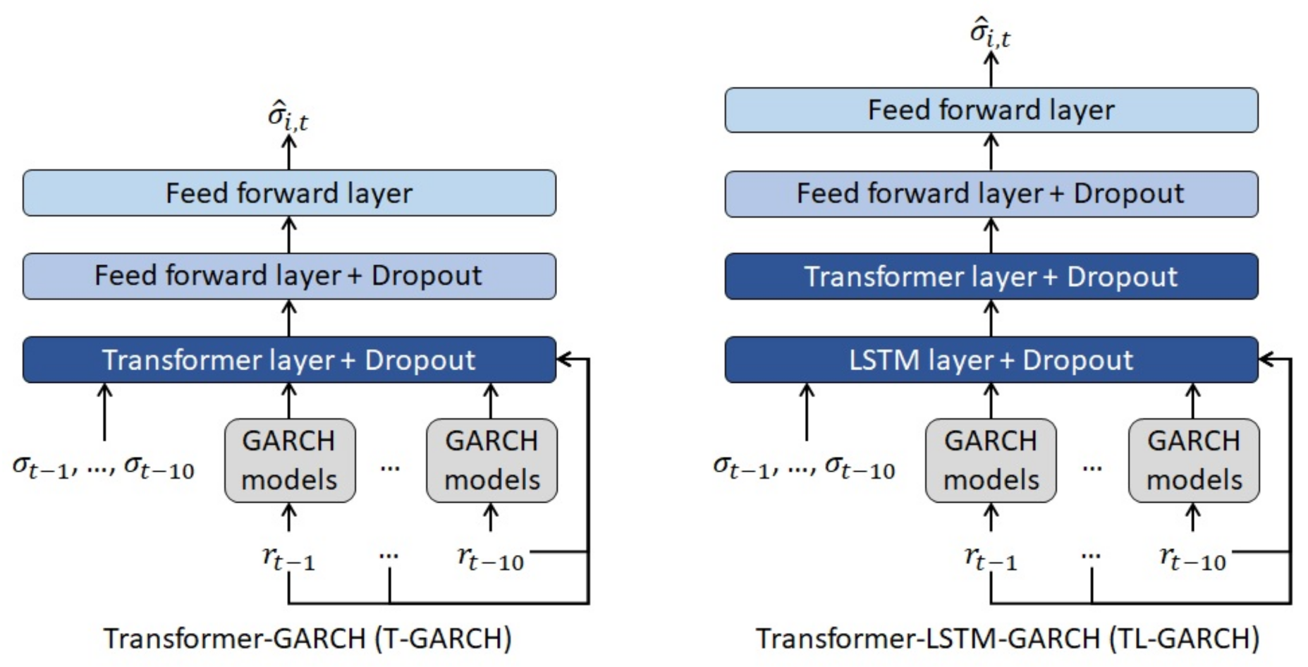
2.4. Transformer-Based Models

Before explaining the volatility models based on Transformer layers (see Figure 3), all the modifications applied to their architecture are presented in this subsection. As previously stated, Transformer layers [54] were developed for NLP purposes. Thus, some modifications are needed in order to apply this layer for volatility forecasting purposes.

In contrast to LSTM, recurrence is not present in the architecture of Transformer layers. The two main components used by these layers in order to deal with time series are the following:

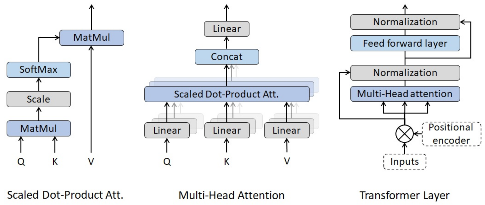
• Positional encoder. As previously stated, Transformer layers have no recurrence structure. Thus, the information about the relative position of the observations within the time series needs to be included in the model. To do so, a positional encoding is added to the input data. In the context of NLP, Vaswani et al. [54] suggested the following wave functions as positional encoders:

  $$\begin{array}{c}P{E}_{(pos,2_i)}=sin(pos/{1000}^{2i/dim})\end{array}$$

  (14)

  $$\begin{array}{c}P{E}_{(pos,2_{i+1})}=cos(pos/{1000}^{2i/dim})\end{array}$$

  (15)

  where $dim$ is the total number of explanatory variables (or word embedding dimension in NLP) used as input in the model, $pos$ is the position of the observation within the time series and $i=(1,2,\cdots ,dim-1)$. This positional encoder modifies the input data depending on the lag of the time series and the embedding dimension used for the words.
  As volatility models do not use words as inputs, the positional encoder is modified in order to avoid any variation of the inputs depending on the number of time series used as input. Thus, the positional encoder suggested in this paper changes depending on the lag, but it remains the same across the different explanatory variables introduced in the model. As in the previous case, a wave function plays the role of positional encoder:

  $$\begin{array}{c}P{E}_{pos}=cos\left(\pi \frac{pos}{N_{pos}-1}\right)=sin\left(\frac{\pi }{2}+\pi \frac{pos}{N_{pos}-1}\right)\end{array}$$

  (16)

  where $pos=(0,1,\cdots ,N_{pos}-1)$ is the position of the observation within the time series and $N_{pos}$ maximum lag.
• Multi-Head attention. It can be considered the key component of the Transformer layers proposed by [54]. As shown in Figure 3, Multi-Head attention is composed of several scaled dot-product attention units running in parallel. Scaled dot-product attention is computed as follows:

  $$\begin{array}{c}Attention(Q,K,V)=softmax\left(\frac{Q{K}^T}{\sqrt{d_k}}\right)V\end{array}$$

  (17)

  where Q, K and V are input matrices and $d_k$ the number of input variables taken into consideration within the dot-product attention mechanism. Multi-Head attention splits the explicative variables in different groups or `heads’ in order to run the different scaled dot-product attention units in parallel. Once the different heads are calculated, the outputs are concatenated (Concat operator) and connected to a feed forward layer with linear activation. Thus, the Multi-Head attention mechanism has the following expression:

  $$\begin{array}{c}MultiHead(Q,K,V)=Concat\left(hea{d}_1,\cdots ,hea{d}_h\right)W^O\end{array}$$

  (18)

  $$\begin{array}{c}hea{d}_i=Attention(Q{W}_i^Q,K{W}_i^K,V{W}_i^V)\end{array}$$

  (19)

  where h is the number of heads. It is also worth mentioning that all the matrices of parameters ($W_i^Q$, $W_i^K$, $W_i^V$ and $W^O$) are trained using feed forward layers with linear activations.

In addition to the scaled dot-product and the Multi-Head attention mechanisms, Figure 3 shows the Transformer layers used in this paper. As suggested by [54], the Multi-Head attention is followed by a normalization, a feed forward layer with ReLU activation and, again, a normalization layer. Transformer layers also include two residual connections [66]. Thanks to these connections, the model will decide by itself if the training of some layers needs to be skipped during some phases of the fitting process.

The modified version of Transformer layers explained in the previous paragraphs are used in the volatility models presented in Figure 4. The T-GARCH architecture proposed in this paper merges the six GARCH algorithms presented in Section 2.3 with Transformer and feed forward layers in order to forecast ${\widehat{\sigma }}_{i,t}$. In addition to the previous algorithms and layers, TL-GARCH includes a LSTM with 32 units. In this last model, the temporal structure of the data is recognized and modelled by the LSTM layer and, thus, no positional encoder is needed in the Transformer layer. Both models have the following characteristics:

• Adaptative Moment Estimator (ADAM) is the algorithm used for updating the weights of the feed forward, LSTM and Transformer layers. This algorithm takes into consideration current and previous gradients in order to implement a progressive adaptation of the initial learning rate. The values suggested by [67] for the ADAM parameters are used in this paper and the initial learning rate is set to $\delta =0.01$.
• The feed forward layers with dropout present in both models have 8 neurons, while the output layer has just one.
• The level of dropout regularization $\theta$ [68] is optimized with the training set mentioned in Section 2.1.
• The loss function used for weights optimization and back propagation purposes is the mean squared error.
• Batch size is equal to 64 and the models are trained during 5000 epochs in order to obtain the final weights.

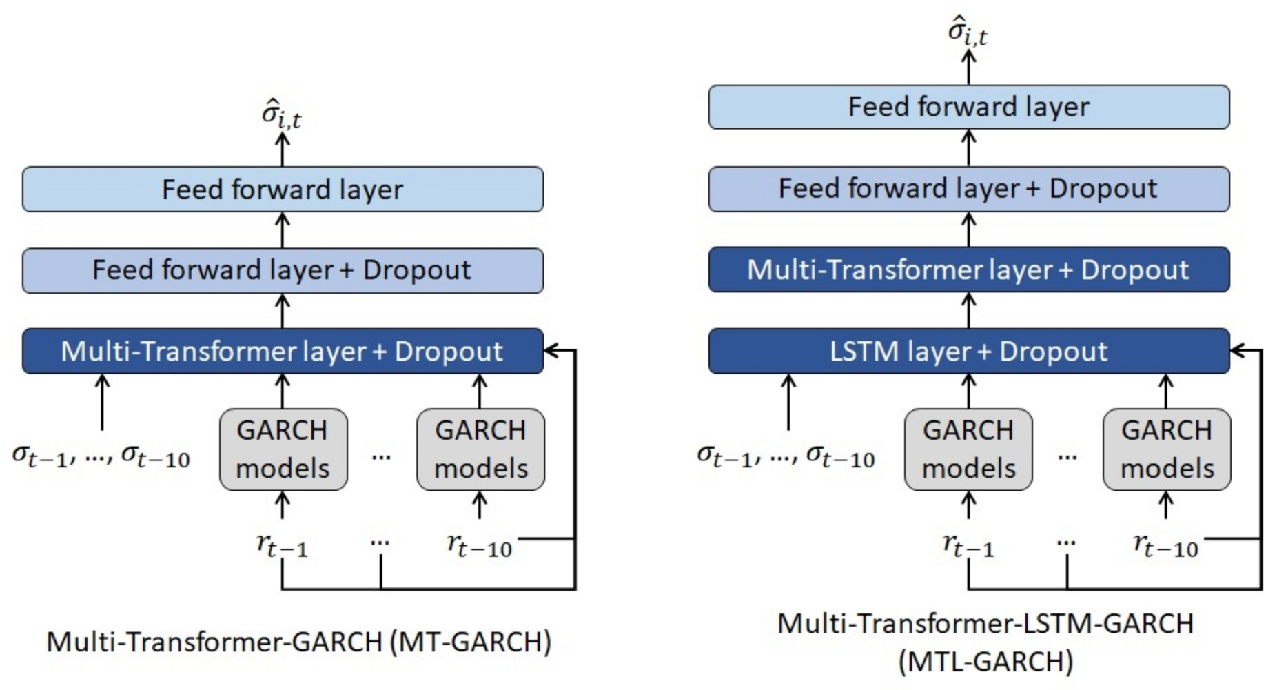
2.5. Multi-Transformer-Based Models

This subsection presents the Multi-Transformer layers and the volatility models based on them. The Multi-Transformer architecture proposed in this paper is a variant of the Transformer layers proposed by [54]. The main differences between both architectures are the following:

• As shown in Figure 5, Multi-Transformer layers generate T different random samples of the input data. In the volatility models proposed in this paper, $90\%$ of the observations of the database are randomly selected in order to compute the different samples.
• Multi-Transformer architecture is composed of T Multi-Head attention units (in this paper $T=5$), one per each random sample of the input data. Then, the average of the different units is computed in order to obtain the final attention matrix. Thus, the Average Multi-Head (AMH) mechanism present in Multi-Transformer can be defined as follows:

  $$\begin{array}{c}AMH(Q,K,V)=\frac{{\sum }_{t=1}^{T}Concat\left(hea{d}_{1,t},\cdots ,hea{d}_{h,t}\right)W_t^O}{T}\end{array}$$

  (20)

  $$\begin{array}{c}hea{d}_{i,t}=Attention(Q_t{W}_{i,t}^Q,K_t{W}_{i,t}^K,V_t{W}_{i,t}^V)\end{array}$$

  (21)

As with the Transformer architecture applied in this paper, the positional encoder used is $P{E}_{pos}$ instead of $P{E}_{(pos,2_i)}$ and $P{E}_{(pos,2_{i+1})}$.

The aim of the Multi-Transformer layers introduced in the paper is to improve the stability and accuracy by applying bagging [69] to the attention mechanism. This technique is usually applied to algorithms such as linear regression, neural networks or decision trees. Instead of applying the procedure on all the data that are input into the model, the proposed methodology uses bagging only to the attention mechanism of the layer architecture.

The computational power required by bagging is one of the main limitations of this technique. As Multi-Transformer applies bagging to the attention mechanisms, their weights are trained several times in each epoch. Nevertheless, bagging is not applied to the rest of the layer weights and, thus, this offsets partially the previous limitation. It is also worth mentioning that bagging preserves the bias and this may result in underfitting.

On the other hand, this technique should bring two main advantages to the Multi-Transformer layer. First, bagging reduces significantly the error variance. Second, the aggregation of learners using this technique leads to a higher accuracy and reduces the risk of overfitting.

The structure of the volatility models based on Multi-Transformer layers (Figure 6) is similar to the architectures presented in Section 2.4. The MT-GARCH merges Multi-Transformer and feed forward layers with the six GARCH models presented in Section 2.3. In addition to the previous algorithms and layers, MTL-GARCH adds a LSTM with 32 units. The rest of the characteristics such as the optimizer, the number of neurons of the feed forward layers or the level of dropout regularization are the same than those presented in the previous section for T-GARCH and TL-GARCH.

The risk measures of ANN-GARCH, LSTM-GARCH and all the models introduced by this paper (Section 2.4 and Section 2.5) are calculated assuming that daily log-returns follow a non-standardize Student’s t-distribution with standard deviation equal to the forecasts made by the volatility models. It is worth mentioning that Student’s t-distribution generates more appropriate risk measures than normal distribution due to the shape of its tail [70,71]. In addition, this assumption is in line with the GARCH-based models used as benchmark and the inputs of the hybrid models presented in this paper.

3. Results

In this section, the forecasts and the risk measures of the volatility models presented in previous sections are compared with the ones obtained from the benchmark models. In addition, the following subsection shows the optimum hyperparameters of the benchmark and proposed hybrid volatility models.

3.1. Fitting of Models Based on Neural Networks

As explained in Section 2.1, rolling window approach ([57,58,59,60] among others) is applied for fitting the algorithms. The training set used for optimizing the level of dropout regularization contains S&P returns and observed volatilities from 1 January 2008 to 31 December 2015.

Table 1. RMSE by level of $\theta$.

Model	$\mathit{\theta }=0$	$\mathit{\theta }=0.05$	$\mathit{\theta }=0.10$	$\mathit{\theta }=0.15$
ANN-GARCH	0.0351	0.0092	0.0085	0.0082
LSTM-GARCH	0.0065	0.0057	0.0056	0.0054
T-GARCH	0.0089	0.0076	0.0072	0.0074
TL-GARCH	0.0050	0.0045	0.0044	0.0045
MT-GARCH	0.0068	0.0062	0.0064	0.0064
MTL-GARCH	0.0047	0.0045	0.0042	0.0044

Source: own elaboration.

presents the error by model and level of $\theta$.

The results of the optimization process reveals that $\theta =0$ generates higher error rates than the rest of the possible values regardless of the model. This means that models based on architectures such as Transformer, LSTM or feed forward layers need an appropriate level of regularization in order to avoid overfitting. According to the results, this is especially relevant for ANN-GARCH, where the error strongly depends on the level of regularization. The dropout level that minimizes the error of each model is selected.

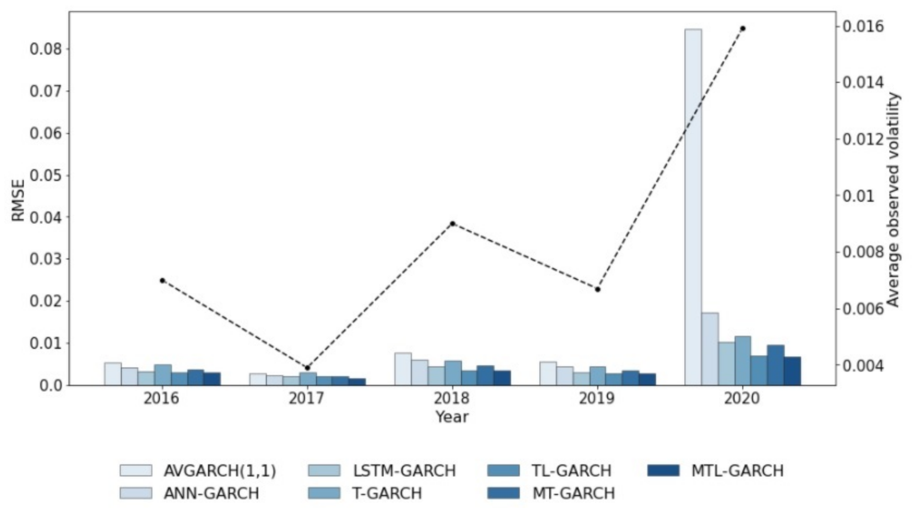
3.2. Comparison against Benchmark Models

Once the optimum dropout level of each of the proposed volatility forecasting models based on Transformer and Multi-Transformer is selected, their performance is compared with the benchmark models (traditional GARCH processes, ANN-GARCH and LSTM-GARCH) presented in Section 2.3.

Table 2. RMSE by volatility model and year.

Model	2016	2017	2018	2019	2020	Total
GARCH(1,1)	0.0058	0.0026	0.0095	0.0073	0.1026	0.0464
AVGARCH(1,1)	0.0053	0.0027	0.0076	0.0056	0.0847	0.0383
EGARCH(1,1)	0.0056	0.0028	0.0093	0.0078	0.0880	0.0399
GJR-GARCH(1,1,1)	0.0090	0.0028	0.0126	0.0068	0.1248	0.0565
TrGARCH(1,1,1)	0.0074	0.0027	0.0115	0.0058	0.1153	0.0521
FIGARCH(1,1)	0.0062	0.0029	0.0095	0.0066	0.1011	0.0457
ANN-GARCH	0.0042	0.0023	0.0060	0.0044	0.0171	0.0086
LSTM-GARCH	0.0032	0.0021	0.0043	0.0030	0.0101	0.0054
T-GARCH	0.0048	0.0029	0.0058	0.0044	0.0117	0.0067
TL-GARCH	0.0030	0.0019	0.0033	0.0026	0.0070	0.0040
MT-GARCH	0.0036	0.0021	0.0046	0.0033	0.0096	0.0054
MTL-GARCH	0.0030	0.0016	0.0033	0.0026	0.0066	0.0038

Source: own elaboration.

and

Table 3. MAE by volatility model and year.

Model	2016	2017	2018	2019	2020	Total
GARCH(1,1)	0.0037	0.0019	0.0058	0.0044	0.0363	0.0105
AVGARCH(1,1)	0.0034	0.0019	0.0049	0.0037	0.0296	0.0087
EGARCH(1,1)	0.0035	0.0020	0.0060	0.0048	0.0333	0.0100
GJR-GARCH(1,1,1)	0.0048	0.0020	0.0074	0.0042	0.0404	0.0118
TrGARCH(1,1,1)	0.0042	0.0020	0.0069	0.0038	0.0365	0.0107
FIGARCH(1,1)	0.0038	0.0021	0.0055	0.0041	0.0361	0.0104
ANN-GARCH	0.0029	0.0019	0.0038	0.0029	0.0095	0.0042
LSTM-GARCH	0.0022	0.0015	0.0027	0.0021	0.0060	0.0029
T-GARCH	0.0035	0.0021	0.0041	0.0031	0.0070	0.0040
TL-GARCH	0.0020	0.0014	0.0021	0.0018	0.0044	0.0023
MT-GARCH	0.0024	0.0016	0.0031	0.0023	0.0057	0.0030
MTL-GARCH	0.0019	0.0012	0.0021	0.0018	0.0041	0.0022

Source: own elaboration.

present the validation error (RMSE and MAE) by year and model. The column `Total’ shows the error of the whole test period (from 1 January 2016 to 31 December 2020). The main conclusions drawn from the these tables are the following:

• Traditional GARCH processes are outperformed by models based on merging artificial neural network architectures such as feed forward, LSTM or Transformer layers with the outcomes of autoregressive algorithms (also named hybrid models).
• The comparison between ANN-GARCH and the rest of the volatility forecasting models based on artificial neural networks (LSTM-GARCH, T-GARCH, TL-GARCH, MT-GARCH and MTL-GARCH) reveals that feed forward layers lead to less accurate forecasts than other architectures. Multi-Transformer, Transformer and LSTM were specially created to forecast time series and, thus, the volatility models based on these layers are more accurate than ANN-GARCH.
• Merging Multi-Transformer and Transformer layers with LSTMs leads to more accurate predictions than traditional LSTM-based architectures. Indeed, TL-GARCH achieves better results than LSTM-GARCH, even though the number of weights of TL-GARCH is significantly lower. Thus, the novel Transformer and Multi-Transformer layers introduced for NLPs purposes can be adapted as described in Section 2.4 and Section 2.5 in order to generate more accurate volatility forecasting models. It is also worth mentioning that Multi-Transformer layers, which were also introduced in this paper, lead to more accurate forecasts thanks to their ability to average several attention mechanisms. In fact, the model that achieves the lower MAE and RMSE is a mixture of Multi-Transformer and LSTM layers (MTL-GARCH).

To enhance the analysis of the results shown in Table 2 and Table 3, Figure 7 collects the RMSE and the observed volatility by year. Notice that only the most accurate GARCH-based model is shown in order to improve the visualization of the graph. The black dashed line shows that the observed volatility of 2020 was significantly higher than the rest of the years due to the turmoil caused by COVID-19 outbreak. As expected, the error of every model is also higher in 2020 because the market volatility was more unpredictable than the rest of the years. Nevertheless, it has to be mentioned that the 2020 forecasts of traditional autoregressive algorithms are significantly less accurate than hybrid models based on architectures such as LSTM, Transformer or Multi-Transformer layers.

Although the observed volatility is lower in years before 2020, autoregressive models are also outperformed by hybrid models. Nevertheless, the difference between both sets of models is remarkably lower.

The p-values of the Kupiec and Christoffersen tests by volatility model and year are shown in

Table 4. Kupiec test (p-values) by volatility model and year.

Model	2016	2017	2018	2019	2020	Total
GARCH(1,1)	0.543	0.540	0.051	0.543	0.052	0.008
AVGARCH(1,1)	0.543	0.540	0.051	0.543	0.052	0.008
EGARCH(1,1)	0.543	0.540	0.051	0.543	0.052	0.008
GJR-GARCH(1,1,1)	0.543	0.540	0.011	0.543	0.190	0.008
TrGARCH(1,1,1)	0.543	0.540	0.051	0.810	0.190	0.042
FIGARCH(1,1)	0.543	0.540	0.051	0.543	0.052	0.008
ANN-GARCH	0.543	0.540	0.001	0.002	0.012	0.001
LSTM-GARCH	0.810	0.186	0.540	0.188	0.190	0.042
T-GARCH	0.188	0.540	0.002	0.543	0.052	0.001
TL-GARCH	0.543	0.540	0.813	0.810	0.810	0.782
MT-GARCH	0.112	0.540	0.540	0.188	0.052	0.089
MTL-GARCH	0.543	0.113	0.113	0.810	0.190	0.910

Source: own elaboration.

and

Table 5. Christoffersen test (p-values) by volatility model and year.

Model	2016	2017	2018	2019	2020	Total
GARCH(1,1)	0.522	0.520	0.004	0.523	0.048	0.002
AVGARCH(1,1)	0.522	0.520	0.004	0.523	0.048	0.002
EGARCH(1,1)	0.522	0.520	0.004	0.523	0.048	0.002
GJR-GARCH(1,1,1)	0.522	0.520	0.002	0.523	0.179	0.002
TrGARCH(1,1,1)	0.522	0.520	0.004	0.800	0.179	0.009
FIGARCH(1,1)	0.522	0.520	0.004	0.523	0.048	0.002
ANN-GARCH	0.522	0.520	0.001	0.002	0.002	0.001
LSTM-GARCH	0.800	0.180	0.520	0.177	0.179	0.037
T-GARCH	0.176	0.520	0.001	0.523	0.048	0.001
TL-GARCH	0.522	0.520	0.803	0.800	0.797	0.693
MT-GARCH	0.113	0.520	0.520	0.177	0.048	0.079
MTL-GARCH	0.522	0.113	0.113	0.800	0.179	0.790

Source: own elaboration.

, respectively. In contrast to the approach suggested by Kupiec, Christoffersen test is not only focused on the total number of exceedances, but it also takes into consideration the number of consecutive VaR exceedances. As stated in Section 2.2, the risk measure and confidence level ($99.5\%$ VaR) selected are in line with Solvency II Directive. This regulation sets the principles for calculating the capital requirements and assessing the risk profile of the insurance companies based in the European Union. This law covers not only the underwriting risks but also financial risks such as the potential losses due to variations on the interest rate curves or the equity prices.

The column ‘Total’ of Table 4 and Table 5 reveal that only TL-GARCH, MT-GARCH and MTL-GARCH produce appropriate risk measures (p-value higher than 0.05 in both tests) for the period 2016–2020. The rest of the models fail both tests and, thus, their risk measures can not be considered to be appropriate for that period.

As with any other statistical test, the higher the number of data points the more relevant are the outcomes obtained from the test. That is the reason why the previous paragraph focuses on the ‘Total’ column and not on the specific results obtained by year. The results by year show that most of the models fail the test in 2020 due to the high level of volatility produced by COVID-19 pandemic.

According to these results, the stock volatility models introduced in this paper (T-GARCH, TL-GARCH, MT-GARCH and MTL-GARCH) produce more accurate estimations and appropriate risk measures in most of the cases. Regarding the models accuracy, it is specially remarkable the difference observed in 2020, where COVID-19 caused a significant turmoil in the stock market. Concerning the appropriateness of equity risk measures, three out of four models based on Transformer and Multi-Transformer pass Kupiec and Christofferesen test for the period 2016–2020, while all the benchmark models fail at least one of them. Notice that the proposed models are compared with other approaches belonging to its own family (ANN-GARCH and LSTM-GARCH) and autoregressive models belonging to the GARCH family.

4. Discussion

This paper introduced a set of volatility forecasting models based on Transformer and Multi-Transformer layers. As Transformer layers were developed for NLP purposes [54], their architecture is adapted in order to generate stock volatility forecasting models. Multi-Transformer layers, which are introduced by this paper, have the aim of improving the stability and accuracy of Transformer layers by applying bagging to the attention mechanism. The predictive power and risk measures generated by the proposed volatility forecasting models (T-GARCH, TL-GARCH, MT-GARCH and MTL-GARCH) are compared with traditional GARCH processes and other hybrid models based on LSTM and feed forward layers.

Three main outcomes were drawn from the empirical results. First, hybrid models based on LSTM, Transformer or Multi-Transformer layers outperform traditional autoregressive algorithms and hybrid models based on feed forward layers. The validation error by year shows that this difference is more relevant in 2020, when the volatility of S&P500 was significantly higher than in the previous years due to COVID-19 pandemic. Volatility forecasting models are mainly used for pricing derivatives and assessing the risk profile of financial institutions. As the more relevant shocks on the solvency position of financial institutions and derivatives prices are observed in high volatility regimes, the accurateness of these models is particularly important in years such as 2020.

The higher performance of hybrid models have also been demonstrated by [38,39,40,41,42,43,44]. These papers merged traditional GARCH models with feed forward layers to predict stock market volatility. This type of models have shown also a superior performance in other financial fields such as oil market volatility [48,49] and metals price volatility [46,47]. Notice that this paper does not only present a comparison with traditional autoregressive models, but it also shows that Transformer and Multi-Transformer can lead to more accurate volatility estimations than other hybrid models.

Second, Multi-Transformer layers lead to more accurate volatility forecasting models than Transformer layers. As expected, applying bagging to the attention mechanism has a positive impact on the performance of the models presented in this paper. It is also remarkable that empirical results demonstrate that merging LSTM with Transformer or Multi-Transformer layers has also a positive impact on the models performance. On one hand, the volatility forecasting model based on Multi-Transformer and LSTM (named MTL-GARCH) achieves the best results in the period 2016–2020. On the other hand, the merging of Transfomer with LSTM (TL-GARCH) leads to a lower error rate than the hybrid model based only on LSTM layers (LSTM-GARCH) even though the number of weights of the first model is significantly lower. Thus, the use of Transfomer layers can lead to simpler and more accurate volatility forecasting models. Notice that Transformer layers are already considered the state of art thanks to BERT [55] and GPT-3 [56]. These models have been successfully used for sentence prediction, conversational response generation, sentiment classification, coding and writing fiction, among others.

Third, the results of Kupiec and Christoffersen tests revealed that only the risk estimations made by MTL-GARCH, TL-GARCH and MT-GARCH can be considered as appropriate for the period 2016–2020, whereas traditional autoregressive algorithms and hybrid models based on feed forward and LSTM layers failed, at least, one of the tests. As previously stated, volatility does not play only a key role in risk management but also in derivative valuation models. Thus, using a volatility model that generates appropriate risk measures can lead to more accurate derivatives valuation.

5. Conclusions

Transformer layers are the state of the art in natural language processing. Indeed, the performance of this layer have overcome the performance of any other previous model in this field [56]. As Transformer layers were specially created for natural language processing, they need to be modified in order to be used for other purposes. Probably, this is one of the main reasons why this layer have not been already extended to other fields. This paper provides the modifications needed to apply this layer for stock volatility forecasting purposes. The results shown in this paper demonstrates that Transformer layers can overcome also the performance of the main stock volatility models.

Following the intuition of bagging [69], this paper introduces Multi-Transformer layers. This novel architecture has the aim of improving the stability and accuracy of the attention mechanism, which is the core of Transformer layers. According to the results, it can be concluded that this procedure improves the accuracy of stock volatility models based on Transformer layers.

Leaving aside the comparisons between Transformer and Multi-Transformer layers, the hybrid models based on them have overcome the performance of autoregressive algorithms and other models based on feed forward layers and LSTMs. The architecture of these hybrid models (T-GARCH, TL-GARCH, MT-GARCH and MTL-GARCH) based on Transformer and Multi-Transformer layers is also provided in this paper.

According to the results, it is also worth noticing that the risk estimations based on the previous models are specially appropriate. The VaR of most of these models can be considered accurate even in years such as 2020, when the COVID-19 pandemic caused a remarkable turmoil in the stock market.

Consequently, the empirical results obtained with the hybrid models based on Transfomer and Multi-Transformer layers suggest that further investigation should be conducted about the possible application of them for derivative valuation purposes. Notice that volatility plays a key role in the financial derivatives valuation. In addition, the models can be extended by merging Transformer or Multi-Transformer layers with other algorithms (such as gradient boosting with trees or random forest) or modifying some key assumptions of the attention mechanism.

References

1. Hull, J. Risk Management and Financial Institutions, 4th ed.; Wiley and Sons: London, UK, 2015. [Google Scholar]
2. Rajashree, P.; Ranjeeeta, B. A differential harmony search based hybrid internal type2 fuzzy EGARCH model for stock market volatility prediction. Int. J. Approx. Reason. 2015, 59, 81–104. [Google Scholar]
3. Engle, R. Autoregressive conditional heteroscedasticity with estimates of the variance of United Kingdom inflation. Econometrica 1982, 50, 987–1007. [Google Scholar] [CrossRef]
4. Bollerslev, T. Generalized autoregressive conditional heteroskedasticity. J. Econom. 1986, 31, 307–327. [Google Scholar] [CrossRef] [Green Version]
5. Mandelbrot, B. The variation of certain speculative prices. J. Bus. 1963, 36, 394–419. [Google Scholar] [CrossRef]
6. Engle, R.; Lee, G. A permanent and transitory component model of stock return volatility. In Cointegration, Causality, and Forecasting: A Festschrift in Honor of Clive W. J. Granger; Engle, R., White, H., Eds.; Oxford University Press: Oxford, UK, 1999; pp. 475–497. [Google Scholar]
7. Haas, M.; Mittnik, S.; Paolella, M. Mixed normal conditional heteroskedasticity. J. Financ. Econom. 2004, 2, 211–250. [Google Scholar] [CrossRef]
8. Haas, M.; Mittnik, S.; Paolella, M. A new approach to Markov-switching GARCH models. J. Financ. Econom. 2004, 2, 493–530. [Google Scholar] [CrossRef]
9. Haas, M.; Paolella, M. Mixture and regime-switching GARCH models. In Handbook of Volatility Models and Their Applications; Bauwens, L., Hafner, C., Laurent, S., Eds.; John Wiley and Sons: Hoboken, NJ, USA, 2012; pp. 71–102. [Google Scholar]
10. Nelson, D.B. Conditional Heteroskedasticity in Asset Returns: A New Approach. Econometrica 1991, 59, 347–370. [Google Scholar] [CrossRef]
11. Glosten, L.; Jagannathan, R.; Runkle, D. On the Relation between the Expected Value and the Volatility of the Nominal Excess Return on Stocks. J. Financ. 1993, 48, 1779–1801. [Google Scholar] [CrossRef]
12. Kraft, D.; Engle, R. Autoregressive Conditional Heteroskedasticity in Multiple Time Series; Department of Economics, UCSD: San Diego, CA, USA, 1982. [Google Scholar]
13. Engle, R.; Granger, C.; Kraft, D. Combining competing forecasts of inflation with a bivariate ARCH model. J. Econ. Dyn. Control. 1984, 8, 151–165. [Google Scholar] [CrossRef]
14. Bollerslev, T.; Engle, R.; Wooldridge, J. A Capital Asset Pricing Model with time-varying covariances. J. Political Econ. 1988, 96, 116–131. [Google Scholar] [CrossRef]
15. Tse, Y.; Tsui, K. A multivariate GARCH model with time-varying correlations. J. Bus. Econ. Stat. 2002, 20, 351–362. [Google Scholar] [CrossRef]
16. Engle, R. Dynamic conditional correlation: A simple class of multivariate generalized autoregressive conditional heteroskedasticity models. J. Bus. Econ. Stat. 2002, 20, 339–350. [Google Scholar] [CrossRef]
17. Engle, R.; Kroner, F. Multivariate simultaneous generalized ARCH. Econom. Theory 1995, 11, 122–150. [Google Scholar] [CrossRef]
18. Engle, R.; Ng, V.; Rotschild, M. Asset pricing with a factor-ARCH covariance structure: Empirical estimates for Treasury Bills. J. Econom. 1990, 45, 213–238. [Google Scholar] [CrossRef] [Green Version]
19. Zhang, L.; Zhu, K.; Ling, S. The ZD-GARCH model: A new way to study heteroscedasticity. J. Econom. 2018, 202, 1–17. [Google Scholar] [CrossRef]
20. Heston, S.L. A closed-form solution for options with stochastic volatility with applications to bond and currency options. Rev. Financ. Stud. 1993, 6, 327–343. [Google Scholar] [CrossRef] [Green Version]
21. Cox, J.; Ingersoll, J.; Ross, S. A Theory of the Term Structure of Interest Rates. Econometrica 1985, 53, 385–407. [Google Scholar] [CrossRef]
22. Melino, A.; Turnbull, S. Pricing foreign currency options with stochastic volatility. J. Econom. 1990, 45, 239–265. [Google Scholar] [CrossRef]
23. Andersen, T.; Sorensen, B. GMM estimation of a stochastic volatility model: A Monte Carlo study. J. Bus. Econ. Stat. 1999, 14, 329–352. [Google Scholar]
24. Durbin, J.; Koopman, S. Monte Carlo maximum likelihood estimation for non-Gaussian state space models. Biometrika 1997, 84, 669–684. [Google Scholar] [CrossRef] [Green Version]
25. Broto, C.; Ruiz, E. Estimation methods for stochastic volatility models: A survey. J. Econ. Surv. 2004, 18, 613–649. [Google Scholar] [CrossRef] [Green Version]
26. Danielsson, J. Stochastic volatility in asset prices: Estimation by simulated maximum likelihood. J. Econom. 2004, 64, 375–400. [Google Scholar] [CrossRef]
27. Andersen, T. Encyclopedia of Complexity and System Sciences; Chapter Stochastic Volatility; Springer: Berlin/Heidelberg, Germany, 2009. [Google Scholar]
28. Hull, J.C.; White, A. The Pricing of Options on Assets with Stochastic Volatilities. J. Financ. 1987, 42, 281–300. [Google Scholar] [CrossRef]
29. Hagan, P.; Kumar, D.; Lesniewski, A.; Woodward, D. Managing Smile Risk. Wilmott Mag. 2002, 1, 84–108. [Google Scholar]
30. Mcculloch, W.; Pitts, W. A Logical Calculus of Ideas Immanent in Nervous Activity. Bull. Math. Biophys. 1943, 5, 127–147. [Google Scholar] [CrossRef]
31. Friedman, J.H. Greedy Function Approximation: A Gradient Boosting Machine. Ann. Stat. 2000, 29, 1189–1232. [Google Scholar]
32. Breiman, L. Random Forests. Mach. Learn. 2001, 45, 5–32. [Google Scholar] [CrossRef] [Green Version]
33. Cortes, C.; Vapnik, V. Support-Vector Networks. Mach. Learn. 1995, 20, 273–297. [Google Scholar] [CrossRef]
34. Gestel, T.; Suykens, J.; Baestens, D.; Lambrechts, A.; Laneknet, G. Financial time series prediction using least squares Support Vector Machines within the evidence framework. IEEE Trans. Neural Netw. 2001, 12, 809–821. [Google Scholar] [CrossRef] [PubMed] [Green Version]
35. Gupta, A.; Dhinga, B. Stock markets prediction using hidden Markov models. In Proceedings of the 2012 Students Conference on Engineering and Systems, Allahabad, India, 16–18 March 2012; pp. 1–4. [Google Scholar]
36. Dias, F.; Nogueira, R.; Peixoto, G.; Moreira, W. Decision-making for financial trading: A fusion approach of Machine Learning and Portfolio Selection. Expert Syst. Appl. 2019, 115, 635–655. [Google Scholar]
37. Hamid, S.; Iqbid, Z. Using neural networks for forecasting volatility of S&P 500 Index futures prices. J. Bus. Res. 2002, 57, 1116–1125. [Google Scholar]
38. Roh, T. Forecasting the Volatility of Stock Price Index. Expert Syst. Appl. 2006, 33, 916–922. [Google Scholar]
39. Hajizadeh, E.; Seifi, A.; Zarandi, F.; Turksen, I. A hybrid modeling approach for forecasting the volatility of S&P 500 Index return. Expert Syst. Appl. 2012, 39, 531–536. [Google Scholar]
40. Kristjanpoller, W.; Fadic, A.; Minutolo, M. Volatility forecast using hybrid neural network models. Expert Syst. Appl. 2014, 41, 2437–2442. [Google Scholar] [CrossRef]
41. Monfared, S.A.; Enke, D. Volatility Forecasting Using a Hybrid GJR-GARCH Neural Network Model. Procedia Comput. Sci. 2014, 36, 246–253. [Google Scholar] [CrossRef] [Green Version]
42. Lu, X.; Que, D.; Cao, G. Volatility Forecast Based on the Hybrid Artificial Neural Network and GARCH-type Models. Procedia Comput. Sci. 2016, 91, 1044–1049. [Google Scholar] [CrossRef] [Green Version]
43. Kim, H.; Won, C. Forecasting the volatility of stock price index: A hybrid model integrating LSTM with multiple GARCH-type models. Expert Syst. Appl. 2018, 103, 25–37. [Google Scholar] [CrossRef]
44. Back, Y.; Kim, H. ModAugNet: A new forecasting framework for stock market index value with an overfitting prevention LSTM module and a prediction LSTM module. Expert Syst. Appl. 2018, 113, 457–480. [Google Scholar] [CrossRef]
45. Bildirici, M.; Ersin, O. Improving forecasts of GARCH family models with the artificial neural networks: An applicaiton to the daily returns in Istanbul Stock Exchange. Expert Syst. Appl. 2009, 36, 7355–7362. [Google Scholar] [CrossRef]
46. Kristjanpoller, W.; Minutolo, M. Gold price volatility: A Forecasting approach using the Artificial Neural Network-GARCH model. Expert Syst. Appl. 2015, 42, 7245–7251. [Google Scholar] [CrossRef]
47. Kristjanpoller, W.; Hernández, E. Volatility of main metals forecasted by a hybrid ANN-GARCH model with regressors. Expert Syst. Appl. 2017, 84, 290–300. [Google Scholar] [CrossRef]
48. Kristjanpoller, W.; Minutolo, M. Forecasting volatility of oil price using an Artificial Neural Network-GARCH model. Expert Syst. Appl. 2016, 65, 233–241. [Google Scholar] [CrossRef]
49. Verma, S. Forecasting volatility of crude oil futures using a GARCH–RNN hybrid approach. Intell. Syst. Accounting, Financ. Manag. 2021. [Google Scholar] [CrossRef]
50. Ramos-Pérez, E.; Alonso-González, P.; Núñez-Velázquez, J. Forecasting volatility with a stacked model based on a hybridized Artificial Neural Network. Expert Syst. Appl. 2019, 129, 1–9. [Google Scholar] [CrossRef]
51. Vidal, A.; Kristjanpoller, W. Gold volatility prediction using a CNN-LSTM approach. Expert Syst. Appl. 2020, 157. [Google Scholar] [CrossRef]
52. Jung, G.; Choi, S.Y. Forecasting Foreign Exchange Volatility Using Deep Learning Autoencoder-LSTM Techniques. Complexity 2021, 2021, 1–16. [Google Scholar] [CrossRef]
53. Peng, Y.; Melo, P.; Camboim de Sá, J.; Akaishi, A.; Montenegro, M. The best of two worlds: Forecasting high frequency volatility for cryptocurrencies and traditional currencies with Support Vector Regression. Expert Syst. Appl. 2018, 97, 177–192. [Google Scholar] [CrossRef]
54. Vaswani, A.; Shazeer, N.; Parmar, N.; Uszkoreit, J.; Jones, L.; Gomez, A.N.; Kaiser, L.; Polosukhin, I. Attention Is All You Need. Adv. Neural Inf. Process. Syst. 2017, 2017, 5998–6008. [Google Scholar]
55. Devlin, J.; Chang, M.; Lee, K.; Toutanova, K. BERT: Pre-training of Deep Bidirectional Transformers for Language Understanding. arXiv 2018, arXiv:1810.04805. [Google Scholar]
56. Brown, T.B.; Mann, B.; Ryder, N.; Subbiah, M.; Kaplan, J.; Dhariwal, P.; Neelakantan, A.; Shyam, P.; Sastry, G.; Askell, A.; et al. Language Models are Few-Shot Learners. In Advances in Neural Information Processing Systems; Larochelle, H., Ranzato, M., Hadsell, R., Balcan, M.F., Lin, H., Eds.; Curran Associates, Inc.: New York, NY, USA, 2020; Volume 33, pp. 1877–1901. [Google Scholar]
57. Swanson, N.R. Money and output viewed through a rolling window. J. Monet. Econ. 1998, 41, 455–474. [Google Scholar] [CrossRef]
58. Goyal, A.; Welch, I. Predicting the Equity Premium With Dividend Ratios; NBER Working Papers 8788; National Bureau of Economic Research, Inc.: Cambridge, MA, USA, 2002. [Google Scholar]
59. Zivot, E.; Wang, J. Modeling Financial Time Series with S-PLUS®; Springer: Berlin/Heidelberg, Germany, 2006. [Google Scholar]
60. Molodtsova, T.; Papell, D. Taylor Rule Exchange Rate Forecasting during the Financial Crisis. NBER Int. Semin. Macroecon. 2012, 9, 55–97. [Google Scholar] [CrossRef] [Green Version]
61. Kupiec, P.H. Techniques for Verifying the Accuracy of Risk Measurement Models. J. Deriv. 1995, 3, 73–84. [Google Scholar] [CrossRef]
62. Christoffersen, P.F.; Bera, A.; Berkowitz, J.; Bollerslev, T.; Diebold, F.; Giorgianni, L.; Hahn, J.; Lopez, J.; Mariano, R. Evaluating Interval Forecasts. Int. Econ. Rev. 1997, 39, 841–862. [Google Scholar] [CrossRef]
63. Bauwens, L.; Hafner, C.; Laurent, S. Handbook of Volatility Models and Their Applications; Wiley Handbooks in Financial E; Wiley: Hoboken, NJ, USA, 2012. [Google Scholar]
64. Taylor, S.J. Modelling Financial Time Series; Wiley: Hoboken, NJ, USA, 1986. [Google Scholar]
65. Baillie, R.T.; Bollerslev, T.; Mikkelsen, H.O. Fractionally integrated generalized autoregressive conditional heteroskedasticity. J. Econom. 1996, 74, 3–30. [Google Scholar] [CrossRef]
66. He, K.; Zhang, X.; Ren, S.; Sun, J. Deep Residual Learning for Image Recognition. In Proceedings of the 2016 IEEE Conference on Computer Vision and Pattern Recognition (CVPR), Las Vegas, NV, USA, 27–30 June 2016; pp. 770–778. [Google Scholar] [CrossRef] [Green Version]
67. Kingma, D.P.; Ba, J. Adam: A Method for Stochastic Optimization. arXiv 2014, arXiv:1412.6980. [Google Scholar]
68. Srivastava, N.; Hinton, G.; Krizhevsky, A.; Sutskever, I.; Salakhutdinov, R. Dropout: A Simple Way to Prevent Neural Networks from Overfitting. J. Mach. Learn. Res. 2014, 15, 1929–1958. [Google Scholar]
69. Breiman, L. Bagging Predictors. Mach. Learn. 1996, 24, 123–140. [Google Scholar] [CrossRef] [Green Version]
70. Jeremic, Z.; Terzić, I. Empirical estimation and comparison of Normal and Student T linear VaR on the Belgrade Stock Exchange. In Proceedings of the Sinteza 2014—Impact of the Internet on Business Activities in Serbia and Worldwide, Belgrade, Serbia, 25–26 April 2014; pp. 298–302. [Google Scholar] [CrossRef] [Green Version]
71. McNeil, A.J.; Frey, R.; Embrechts, P. Quantitative Risk Management: Concepts, Techniques and Tools; Princeton University Press: Princeton, NJ, USA, 2015. [Google Scholar]
Figure 1. Rolling window methodology.
Mathematics 09 01794 g001
Figure 2. ANN-GARCH and LSTM-GARCH architectures.
Mathematics 09 01794 g002
Figure 3. Transformer and Multi-Head attention mechanism.
Mathematics 09 01794 g003
Figure 4. T-GARCH and TL-GARCH volatility models.
Mathematics 09 01794 g004
Figure 5. Multi-Transformer architecture.
Mathematics 09 01794 g005
Figure 6. MT-GARCH and MTL-GARCH volatility models.
Mathematics 09 01794 g006
Figure 7. Observed volatility and RMSE by year.
Mathematics 09 01794 g007