Emergency Quantity Discount Contract with Suppliers Risk Aversion under Stochastic Price

Abstract

This paper constructs an emergency quantity discount contract to explore the inherent law of the contract coordinating the supply chain with stochastic market demand and price and the risk-averse supplier. Meanwhile, the conditional value-at-risk (CVaR) risk measure criterion is revised to study the influence of supplier’s risk aversion attitude on supply chain coordination. The results show that supplier risk aversion will cause the bifurcation of the relevant factors in the supply chain under the stochastic price. Within the bifurcation region, the supply chain cannot be coordinated; out of the bifurcation region, the supply chain can achieve coordination. The supply chain related factors’ variation range in the bifurcation region is related to the step size of the risk aversion factor and the normal distribution function’s variance of the market demand, and it increases with the latter.

1. Introduction

The use of contracts to coordinate the supply chain is an important research field in the current supply chain management field. There are many types of supply chain contracts. A quantity discount contract is the most commonly used one, and it has many forms. The quantity discount contract in this paper refers to an agreement in which the unit wholesale price provided by the supplier is inversely proportional to the retailer’s order quantity. The contract is mainly used for small profits, but the quick turnover of industrial products or time-sensitive fresh agricultural and sideline products or seasonal clothing industries.

The initial research on the use of quantity discount contract to coordinate supply chains was mostly carried out on the premise of fixed market prices and a stable market external environment. Monahan [1] took the lead in researching quantity discount contract. Cachon [2] applied quantity discount contract to coordinate the simplest secondary supply chain. Huang et al. [3] introduced quantity discount contracts to restrain retailers’ potential incentives to encourage returns. Sun et al. [4] investigated the effectiveness of quantity discount contracts in slowing down the spread of bankruptcies among supply chain members. Ogier et al. [5] proposed a batch model integrating quantity discounts for local planning problems. Kwong et al. [6] used Stackelberg game theory to establish a joint optimization model of manufacturers and retailers considering quantity discount contracts.

The above studies are all about the benchmark quantity discount contract. Later scholars have conducted extensive research on the application of quantity discount contracts in practical problems. The research involves delayed payment, energy, trade credit, transportation, and so on. Yu et al. [7] proposed a power supply chain coordination model based on quantity discount contracts. Sheen and Tsao [8] considered the coordination of the quantity discount contract and delayed payment of the retailer’s transportation cost. Wang and Liu [9] studied the role of trade credit and quantity discounts in supply chain coordination after considering the impact of sales efforts on market demand. Zhang et al. [10] studied the use of quantity discount contracts to coordinate supply chains when there is a risk of trade credit default. Zhou and Kim [11] proposed the optimal concession contract design method between the port authority and two container terminal operators under different quantity discount revenue sharing schemes. Zhang et al. [12] discussed the issue of the multi-period newsvendor problem with stable demand and quantity discounts.

With gradual deepening of research, the scope of study gradually involves supply chain coordination issues under the circumstances of market demand fluctuations and changes in production costs. Peng et al. [13] explored the quantity discount contract model of the fashion supply chain under uncertain income and random demand. Zhao et al. [14] investigated the supply chain coordination problem of demand interruption in the fashion supply chain with revenue-sharing contract and linear quantity discount contract. Lee [15] studied the quantity discount contract between the manufacturer and the retailer under a stochastic two-period inventory model. Most of the research mentioned above objects are the most straightforward secondary supply chains, and some scholars have studied more complex supply chains. Nie and Du [16] discussed the quantity discount contract coordination mechanism in a binary supply chain composed of one supplier and two retailers. Huang et al. [17] studied the quantity discount contract to coordinate a supply chain composed of a retailer and multiple suppliers. Zhang et al. [18] considered the fixed life of the product and explored the coordination problem of a production-inventory integrated system with a quantity discount under the condition of limited productivity and deterministic demand. Zheng et al. [19] considered the quantity discount contract of the new product supply chain composed of one supplier and multiple retailers under the two independent procurement and joint procurement cases.

After the 2008 financial crisis, scholars and business managers recognized the importance of supply chain risk management. Scholars have begun to study the problem of diversifying risks when participants are averse to risks due to emergencies under the premise of stable market prices. Agrawal and Seshadri [20] proposed using quantity discount contracts to diversify the losses caused by risk-averse retailers. The research mentioned above mainly studies the methods of diversifying risks without quantitative estimation of risks. Later, many scholars introduced quantitative risk management methods in financial management into supply chain risk management. Liang et al. [21] studied a supply chain system with a risk-neutral manufacturer as the leader and a risk-averse retailer as the follower based on the VaR (value-at-risk) method. Bai and Liu [22] proposed a robust optimization method to solve the supply chain network design problem using the variable probability distribution through the fuzzy VaR modelling method. Rockfellar and Uryasev [23,24] proposed to use conditional value-at-risk (CVaR) as a risk measurement criterion for the limitations of VaR theory. As a result, CVaR has become a popular method for studying supply chain risk management. Tao et al. [25] proposed a CVaR way to measure overdue penalties to incorporate decision-makers risk aversion. Chen et al. [26] established an improved newsboy model with random default probability to reduce the default loss using CVaR as the measurement criterion.

Analyzing the literature shows that some consider the random changes in market prices caused by emergencies, but the supply chain participants remain risk-neutral. Some thought participants’ risk aversion caused by emergencies but did not consider the random fluctuations of market prices. The literature that considers multi-factor disturbances such as random changes in market prices and risk aversion among participants is still relatively rare. Therefore, this paper considers whether the supply chain can be effectively coordinated using quantity discount contracts under the simultaneous disturbance of multiple factors such as random market demand, random market prices, and supplier risk aversion.

In summary, the main contributions of this paper are as follows: (1) Analyze and revise the existing ‘profit-CVaR’ risk measure criteria. (2) Introduce stochastic price into the field of supply chain risk management and construct an emergency quantity discount contract model under multi-factor disturbance. (3) The phenomenon of bifurcation and mutation in supply chain coordination is discovered and analyzed.

The rest of the paper is structured as follows: Section 2 constructs the benchmark quantity discount contract model, the emergency quantity discount contract model under the condition of price stability, and the emergency quantity discount contract model under the stochastic price. In Section 3, the limitations of the existing “profit-CVaR” risk measure criteria are analysed, and relevant proofs are given. On this basis, an emergency quantity discount contract model under the condition of stochastic price and supplier risk aversion is further constructed. Section 4 provides a specific numerical example and analyzes the results of the example in detail. The conclusion is given in Section 5.

2. Quantity Discount Contract Model and Assumptions

2.1. Benchmark Quantity Discount Contract

Take the simplest secondary supply chain as the research object to construct the benchmark quantity discount contract. Let $p_0$ be the market equilibrium price of the product, which is a fixed value. $c_s$ and $c_r$ are the marginal production cost and sales cost of the product, and $c=c_r+c_s$; $g_s$ and $g_r$ are the marginal stock-out loss costs of suppliers and retailers, respectively, and $g=g_r+g_s$. $v$ is the marginal residual value of the missing commodity. $w(q)$ is the wholesale price provided by the supplier, which is inversely proportional to the order quantity $q$. $x$ is the random market demand, and $D(x)$ is the market demand function. Its distribution function and probability density function are $F(x)$ and $f(x)$ respectively, which are continuously differentiable and differentiable. The expectation of the demand function is $E[D(x)]={\displaystyle {\int }_0^{\infty }x}f(x)dx={\mu }_G$ and the expected sales volume is $S(q)=q-{\displaystyle {\int }_0^{q}F(x)}dx$. Assuming that the product is a short-life cycle product and the information between members of the supply chain is completely shared, then:

The retailer’s expected profit function is defined as

$$\begin{array}{l}E{\pi }_r={\displaystyle {\int }_0^q[p_{0}x+v(q-x)]}f(x)dx+{\displaystyle {\int }_q^{\infty }[p_{0}q}-g_r(x-q)]f(x)dx-c_{r}q-w(q)q\\ \hspace{1em}\hspace{1em}=(p_0+g_r-v)S(q)-[w(q)+c_r-v]q-g_{r}u\end{array}$$

(1)

The supplier’s expected profit function is defined as

$$E{\pi }_s=w(q)q-c_{s}q-g_s[\mu -S(q)]=g_{s}S(q)+[w(q)-c_s]q-g_s\mu$$

(2)

The expected profit function of the supply chain is defined as

$$E{\pi }_h=E{\pi }_r+E{\pi }_s=(p_0+g-v)S(q)-(c-v)q-g\mu$$

(3)

2.2. Emergency Quantity Discount Contract under the Condition of Stable Price

When an emergency occurs, it only causes a change in market demand but does not cause a change in market price. Therefore, the distribution function and probability density function become $H(x)$ and $h(x)$. The market demand expectation becomes $E[D(x)]={\displaystyle {\int }_0^{\infty }x}h(x)dx={\mu }_H$, the expected sales becomes $S_H(q)=q-{\displaystyle {\int }_0^{q}H}(x)dx$, the ending inventory becomes $I(q)=q-S_H(q)$, and the shortage becomes $L(q)={\mu }_H-S_h(q)$. After an emergency occurs, when the market demand exceeds the original optimal order quantity, the supplier will expand production, assuming that the marginal production cost of expanding production is ${\lambda }_1$. If the situation is reversed, the number of remaining products will be increased, assuming that the marginal processing cost of these products is ${\lambda }_2$. Based on this, the expected revenue function of the retailer, supplier and supply chain can be obtained respectively:

$$\begin{array}{l}E{\pi }_r^c={\displaystyle {\int }_0^q[p_{0}x+v(q-x)]}h(x)dx+{\displaystyle {\int }_q^{\infty }[p_{0}q}-g_r(x-q)]h(x)dx-c_{r}q-w(q)q\\ \hspace{1em}\hspace{1em}=(p_0-v+g_r)S_H(q)-[w(q)+c_r-v]q-g_r{\mu }_H\end{array}$$

(4)

$$\begin{array}{l}E{\pi }_s^c=w(q)q-{\displaystyle {\int }_q^{\infty }{g}_s}(x-q)h(x)dx-c_{s}q-{\lambda }_1{(q-q^{*})}^{+}-{\lambda }_2{(q^{*}-q)}^{+}\\ \hspace{1em}\hspace{1em}=g_s{S}_H(q)-[c_s-w(q)]q-g_s{\mu }_H-{\lambda }_1{(q-q^{*})}^{+}-{\lambda }_2{(q^{*}-q)}^{+}\end{array}$$

(5)

$$E{\pi }_h^c=E{\pi }_r^c+E{\pi }_s^c=(p_0-v+g)S_F(q)-(c-v)q-g{\mu }_F-{\lambda }_1{(q-q^{*})}^{+}-{\lambda }_2{(q^{*}-q)}^{+}$$

(6)

2.3. Emergency Quantity Discount Contract under the Condition of Stochastic Price

Assume that emergencies cause rapid changes in market supply and demand and cause market prices to change randomly and changes in the relationship between supply and demand. $p$ represents the random market price of the commodity, and satisfies $dp=[p_0+a(x-q)]dx$, where $a$ is the market size coefficient. The market demand distribution function and the probability density function become $G(x)$ and $g(x)$ respectively, the market demand expectation becomes $E[D(x)]={\displaystyle {\int }_0^{\infty }x}g(x)dx={\mu }_G$, and the expected sales becomes $S_G=q-{\displaystyle {\int }_0^{q}G}(x)dx$. Therefore, the ending inventory becomes $I(q)=q-S_G(q)$ and the out-of-stock becomes $L(q)={\mu }_G-S_G(q)$. The expected profit function of retailer, supplier, and supply chain can be expressed as

$$E{\pi }_r^u={\displaystyle {\int }_0^q[[p_0+a(x-q)]x+v(q-x)]}g(x)dx+{\displaystyle {\int }_q^{\infty }[[p_0+a(x-q)]q}-g_r(x-q)]g(x)dx-c_{r}q-w(q)q$$

(7)

$$\begin{array}{l}E{\pi }_s^u=w(q)q-{\displaystyle {\int }_q^{\infty }{g}_s}(x-q)g(x)dx-c_{s}q-{\lambda }_1{(q-q^{*})}^{+}-{\lambda }_2{(q^{*}-q)}^{+}\\ \hspace{1em}\hspace{1em}=g_s{S}_H(q)-[-w(q)+c_s]q-g_s{\mu }_G-\widehat{B(q)}\end{array}$$

(8)

$$E{\pi }_h^u=E{\pi }_r^u+E{\pi }_s^u=(p_0-v+g)S_G(q)-(c-v)q-g{\mu }_G+\widehat{A(q)}-\widehat{B(q)}$$

(9)

where $\widehat{A(q)}={\displaystyle {\int }_0^{q}a}{x}^{2}g(x)dx-{\displaystyle {\int }_0^{q}a}qxg(x)dx+{\displaystyle {\int }_q^{\infty }a}xqg(x)dx-{\displaystyle {\int }_q^{\infty }a}{q}^{2}g(x)dx$ and $\widehat{B(q)}={\lambda }_1{(q-q^{*})}^{+}+{\lambda }_2{(q^{*}-q)}^{+}$.

3. Emergency Quantity Discount Contract of Supplier Risk Aversion under the Condition of Stochastic Price

3.1. Analysis of the Existing ‘Profit-CVaR’ Risk Measure

Conditional value at risk (CVaR) is an investment risk measurement method developed by Rockafella and Uryasev [23,24] based on the value at risk (VaR). It refers to the average loss value of the portfolio loss exceeding a given VaR value. The specific mathematical expression of CVaR is

$$CVa{R}_{\theta }{\pi }_i(x)=E(-X|-X\ge Va{R}_{\theta }{\pi }_i(x))=\frac{1}{\theta }{\displaystyle \underset{{\pi }_i(x)<Va{R}_{\theta {\displaystyle \prod i}(x)}}{\int }{\pi }_i}(x)f(x)dx$$

(10)

where $-\mathrm{X}(\mathrm{x}>0)$ represents random loss, $Va{R}_{\theta }$ is the VaR value with risk factor $\theta$, and ${\pi }_i(x)$ is the profit function.

To simplify the calculation of $CVa{R}_{\theta }{\pi }_i\left(x\right)$, RockafeUar and Uryasev proposed and proved a more general equivalent definition of $CVa{R}_{\theta }{\pi }_i\left(x\right)$

$$CVa{R}_{\theta }{\pi }_i\left(x\right)=\underset{V\in R}{\max }\left\{V-\frac{1}{\theta }E{\left[-{\pi }_i\left(x\right)+V\right]}^{+}\right\}$$

(11)

Many scholars believe that despite the outstanding advantages of the CVaR criterion, it is not difficult to find from its definition that CVaR only reflects the situation where the loss exceeds a given VaR value. In contrast, the case when the profit is higher than the given level is insufficiently considered. Therefore, it is further proposed to take the weighted average of the risk-averse person’s expected profit and CVaR as the measurement criterion, and the maximum measurement criterion is defined as

$$\max \left\{\rho E{\pi }_i(x)+(1-\rho )CVa{R}_{\theta }{\pi }_i(x)\right\}$$

(12)

where $\rho \in [0,1]$.

The analysis shows that although this decision-making method considers the profit of the entire supply chain system while considering the risk, the optimal ordering strategy is derived under decentralized decision-making. Under decentralized decision-making, it is easy to produce double marginalization effects so that the income of supply chain members and the income of the entire supply chain cannot reach Pareto optimal at the same time. Therefore, this paper revises the risk measure criterion under decentralized decision-making to the risk measure criterion under centralized decision-making. This criterion is used to study the supply chain coordination problem under centralized decision-making. The specific expression is defined as

$$\max \left\{E{\pi }_i(x)+CVa{R}_{\mathsf{\Theta }}{\pi }_j(x)\right\}$$

(13)

Proposition 1.

The revised ‘profit-CVaR’ criterion is better than the original ‘profit-CVaR’ criterion in measuring risk. It is manifested in that the optimal order quantity obtained under the revised criterion is not lower than the optimal order quantity obtained under the pre-modified criterion.

Proof. 

Without loss of generality, take the benchmark quantity discount contract as an example to prove it. The expected profit function of the retailer, the expected profit function of the supplier and the expected profit function of the supply chain are respectively

$$\begin{array}{l}E{\pi }_r={\displaystyle {\int }_0^q[p_{0}x++v(q-x)]}f(x)dx+{\displaystyle {\int }_q^{\infty }[p_{0}q}-g_r(x-q)]f(x)dx-c_{r}q-w(q)q\\ \hspace{1em}\hspace{1em}=(p_0+g_r-v)S(q)-[w(q)+c_r-v]q-g_{r}u\end{array}$$

(14)

$$E{\pi }_s=w(q)q-c_{s}q-g_s[\mu -S(q)]=g_{s}S(q)+[w(q)-c_s]q-g_s\mu$$

(15)

$$E{\pi }_h=E{\pi }_r+E{\pi }_s=(p_0+g-v)S(q)-(c-v)q-g\mu$$

(16)

Under centralized decision-making, from Equation (10), we can get

$$\frac{\partial E{\pi }_h}{\partial q}=(p_0+g-v)[1-G(q)]-(c-v)$$

(17)

$$\frac{{\partial }^{2}E{\pi }_h}{\partial q^2}=-(p_0+g-v)g(q)<0$$

(18)

Equation (12) shows that Equation (10) is a strictly concave function. Let Equation (11) be equal to zero, and we can get

$$q_h^{*}=G^{-1}\left[\frac{p_0+g-c}{p_0+g-v}\right]$$

(19)

Under decentralized decision-making, from Equation (10), we can get

$$E{\pi }_s=E{\pi }_h-E{\pi }_r$$

(20)

According to common sense, the retailer has an optimal order quantity, let

$$\frac{\partial E{\pi }_s}{\partial q}=\frac{\partial E{\pi }_h}{\partial q}-\frac{\partial E{\pi }_r}{\partial q}=0$$

(21)

then

$$(p_0+g-v)[1-G(q)]-(c-v)-\frac{\partial E{\pi }_r}{\partial q}=0$$

(22)

$$(p_0+g-v)[1-G(q)]-(c-v)\ge 0$$

(23)

$$q_s^{*}\le G^{-1}[\frac{p_0+g-c}{p_0+g-v}]=q_h^{*}=q^{*}$$

(24)

Let

$$Z(q)=\max \{\rho E{\pi }_s+(1-\rho )[V-\frac{1}{\mathsf{\Theta }}E{\left(V-{\pi }_s\right)}^{+}]\}$$

(25)

Finding the first-order derivative and the second-order derivative of Equation (19), respectively, we can get

$$\frac{dZ(q)}{dq}=(\rho +\frac{1-\rho }{\mathsf{\Theta }})\frac{\partial E{\pi }_s}{\partial q}$$

(26)

$$\frac{d^{2}Z(q)}{d{q}^2}=(\rho +\frac{1-\rho }{\mathsf{\Theta }})\frac{{\partial }^{2}E{\pi }_s}{\partial q^2}<0$$

(27)

From Equation (21), we can see that there is an optimal order quantity. Let Equation (20) be equal to zero, that is, $q_z^{*}$ can be found. The analysis is easy to know that $q_z^{*}=q_s^{*}$.

Further, let

$$Y(q)=\max \{E{\pi }_r(x)+CVa{R}_{\mathsf{\Theta }}{\pi }_s(x)\}=\max \{E{\pi }_r+[V-\frac{1}{\mathsf{\Theta }}E{\left(V-{\pi }_s\right)}^{+}]\}$$

(28)

The same can be obtained: $q_y^{*}=q_h^{*}=q^{*}$. Namely, $q_y^{*}\ge q_z^{*}$.

Therefore, this paper revises the expression of the risk measure criterion as

$$Y(q)=\underset{q}{\max }\{E{\pi }_r(x)+CVa{R}_{\mathsf{\Theta }}{\pi }_s(x)\}$$

(29)

□

3.2. Emergency Quantity Discount Contract Model with Stochastic Price and Supplier Risk Aversion

Under the new assumptions, the revised ‘profit-CVaR’ criterion is used to measure risk. A quantity discount contract model of supplier risk aversion is established under centralized decision-making to coordinate the supply chain. The supplier’s conditional value-at-risk utility function is defined as

$$\begin{array}{l}CVaR({\pi }_s)=\frac{1}{\mathsf{\Theta }}\{w(q)q-{\displaystyle {\int }_q^{\frac{q}{\mathsf{\Theta }}}{g}_s}(x-q)g(x)dx-c_{s}q-{\lambda }_2-{\displaystyle {\int }_{\frac{q}{\mathsf{\Theta }}}^{\infty }{g}_s}(x-\frac{q}{\mathsf{\Theta }})g_s(x-\frac{q}{\mathsf{\Theta }})g(x)dx\\ \hspace{1em}\hspace{1em}\hspace{1em}\hspace{1em}=\frac{1}{\mathsf{\Theta }}[E{\pi }_s^u+g_s{\displaystyle {\int }_{\frac{q}{\mathsf{\Theta }}}^{\infty }(\frac{q}{\mathsf{\Theta }}-q)g(x)}]dx\end{array}$$

(30)

The retailer’s expected return function is defined as

$$\begin{array}{l}E{\pi }_r^u={\displaystyle {\int }_0^q[[p_0+a(x-q)]x+v(q-x)]}g(x)dx+{\displaystyle {\int }_q^{\infty }[[p_0+a(x-q)]q}-g_r(x-q)]g(x)dx-c_{r}q-w(q)q\\ \hspace{1em}\hspace{1em}=(p_0-v+g_r)S_G(q)-[c_r+w(q)-v]q-g_r{\mu }_G+\widehat{A(q)}\end{array}$$

(31)

Find the first derivative of Equation (24) to get

$$\frac{\partial CVaR({\pi }_s)}{\partial q}=\frac{1}{\mathsf{\Theta }}\{\frac{\partial E{\pi }_s^u}{\partial q}+g_s(\frac{1}{\mathsf{\Theta }}-1)[1-G(\frac{q}{\mathsf{\Theta }})]-g_{s}q(\frac{1}{\mathsf{\Theta }}-1)\frac{1}{\mathsf{\Theta }}g(\frac{q}{\mathsf{\Theta }})\}$$

(32)

Find the second derivative of Equation (24) to get

$$\frac{{\partial }^{2}CVaR({\pi }_s)}{\partial q^2}=\frac{1}{\mathsf{\Theta }}\{\frac{{\partial }^{2}E{\pi }_s^u}{\partial q^2}-g_s(\frac{1}{\mathsf{\Theta }}-1)f(\frac{q}{\mathsf{\Theta }})-g_s(\frac{1}{\mathsf{\Theta }}-1)\frac{1}{\mathsf{\Theta }}f(\frac{q}{\mathsf{\Theta }})-g_{s}q(\frac{1}{\mathsf{\Theta }}-1)\frac{1}{{\mathsf{\Theta }}^2}{f}^{’}(\frac{q}{\mathsf{\Theta }})\}<0$$

(33)

It can be seen from Equation (27) that Equation (24) is a strictly concave function, so there is a unique optimal order quantity $q_s^{*}$. Let $\frac{\partial CVaR({\pi }_s)}{\partial q}=0$, the solution obtained is $q_s^{*}$.

Find the first derivative of Equation (25) to get

$$\frac{\partial E{\pi }_r^u}{\partial q}=(p_0+g_r-v)[1-G(q)]-\frac{\partial w(q)}{\partial q}-(c_r+w(q)-v)-\frac{\partial \widehat{A}(q)}{\partial q}$$

(34)

Find the second derivative of Equation (25) to get

$$\frac{{\partial }^{2}E{\pi }_r^u}{\partial q^2}=-(p_0+g_r-v)g(q)-\frac{{\partial }^{2}w(q)}{\partial q^2}-\frac{\partial w(q)}{\partial q}-2a[1-G(q)]<0$$

(35)

It can be seen from Equation (29) that Equation (26) is a strictly concave function, so let $\frac{\partial E{\pi }_r^{\mu }}{\partial q}=0$, we can get the only optimal order quantity $q_r^{*}$. When $q_r^{*}=q_s^{*}=q_h^{*}$, the supply chain system can achieve Pareto optimal and achieve coordination.

4. Numerical Example

Assuming that a company sells certain emergency supplies, the various parameters of the goods under the stable market conditions are: $p_o=300$, $c_r=50$, $c_s=100$, $g_r=10$, $g_s=10$, $v=80$ (see the preceding text for the meaning of the above parameters). Suppose that the market demand under emergencies obeys the distributions $X~N(50,000,{100}^2)$, $X~N(50,000,{80}^2)$, $X~N(50,000,{50}^2)$, and $X~N(50,000,{30}^2)$ respectively. Discuss the influence of the change of the risk aversion factor $\theta$ in the interval $[0.1,1]$ and $[0.91,1]$ with 0.1 and 0.01 as the steps respectively on the optimal order quantity. See

Table 1. Changes of the optimal order quantity in different $\sigma$ when $\theta \in [0.1,1]$.

	σ = 100	σ = 80	σ = 50	σ = 30
θ = 0.1	48,750	48,750	48,750	48,750
θ = 0.2	48,750	48,750	48,750	48,750
θ = 0.3	48,750	48,750	48,750	48,750
θ = 0.4	48,750	48,750	48,750	48,750
θ = 0.5	48,750	48,750	48,750	48,750
θ = 0.6	48,750	48,750	48,750	48,750
θ = 0.7	48,750	48,750	48,750	48,750
θ = 0.8	48,750	48,750	48,750	48,750
θ = 0.9	48,750	48,750	48,750	48,750
θ = 1	48,750	48,750	48,750	48,750

and

Table 2. Changes of the optimal order quantity in different $\sigma$ when $\theta \in [0.91,1]$.

	σ = 100	σ = 80	σ = 50	σ = 30
θ = 0.91	48,750	48,750	48,750	48,750
θ = 0.92	48,750	48,750	48,750	48,750
θ = 0.93	48,750	48,750	48,750	48,750
θ = 0.94	48,750	48,750	48,750	48,750
θ = 0.95	48,750	48,750	48,750	48,750
θ = 0.96	48,750	48,750	48,750	48,750
θ = 0.97	48,846	48,787	48,750	48,750
θ = 0.98	48,702	48,743	48,797	48,801
θ = 0.99	48,775	48,775	48,775	48,775
θ = 1	48,750	48,750	48,750	48,750

for details. The impact of the risk aversion factor $\theta$ in interval $[0.965,1]$ with 0.001 as the step size on various decision variables in the supply chain is shown in Figure 1, Figure 2, Figure 3, Figure 4 and Figure 5.

As can be seen from the data in Table 1, when $\theta$ changes in the interval of $[0.1,1]$ with a step size of 0.1, the optimal order quantity under the risk aversion of the supplier is equal to the optimal order quantity under the risk neutrality of the participants regardless of the variance change. It shows that in this case, both risk aversion and variance have no effect on the performance of the supply chain, and the supply chain can achieve coordination.

It can be seen from Table 2 that in the case of random prices and supplier risk aversion, when $\theta$ changes in the interval $[0.91,1]$ with a step length of 0.01, the optimal order quantity under different variances begins to change. When $\theta$ is equal to 1, it is the same as the optimal order quantity in the risk-neutral case.

The X-axis in Figure 1, Figure 2, Figure 3, Figure 4 and Figure 5 represents the risk aversion factor, that is, the supplier’s risk aversion degree. The Y-axis of Figure 1, Figure 2, Figure 3, Figure 4 and Figure 5 respectively represent the optimal order quantity, retailer’s expected revenue, supplier’s expected revenue, supply chain’s expected revenue, and the value of “${\pi }_s+CVaR({\pi }_r)$”. 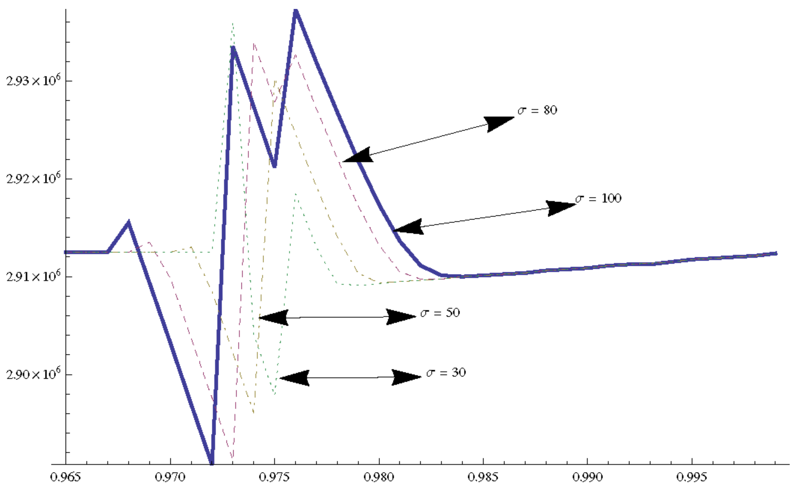Figure 1 shows that when $\sigma =30$ and the risk aversion factor $\theta =0.973$, the retailer’s optimal order quantity begins to change and is no longer equal to 48,750. When $\sigma =50$ the optimal order quantity starts to change when $\theta =0.971$. When $\sigma =80$ and $\theta =0.969$, the optimal order quantity begins to change. When $\sigma =100$, the optimal order quantity starts to change at $\theta =0.967$. From the above changes, it can be seen that the optimal order quantity under the coordination of the quantity discount contract will vary with the evolution of the risk aversion factor. However, when the risk aversion factor tends to 1, the optimal order quantity under different market demand distributions will gradually align with the optimal order quantity under risk-neutral conditions.

In addition, when $\sigma =30$, the optimal order quantity $q^{*}$ begins to show bifurcation mutation from $\theta =0.973$, and the change interval of $q^{*}$ is $[48,561,48,867]$. The value of $q^{*}$ is the smallest when $\theta =0.973$ and the largest when $\theta =0.975$. When $\sigma =50$, the optimal order quantity $q^{*}$ begins to show a bifurcating mutation from $\theta =0.971$, and the change interval of $q^{*}$ is $[48,607,48,881]$, and the value of $q^{*}$ is the smallest when $\theta =0.975$ and the largest when $\theta =0.973$. When $\sigma =80$, the optimal order quantity $q^{*}$ begins to show bifurcation mutation from $\theta =0.969$, and the change interval of $q^{*}$ is $[48,588,49,017]$, and the value of $q^{*}$ is the smallest when $\theta =0.976$ and the largest when $\theta =0.975$. When $\sigma =100$, the optimal order quantity $q^{*}$ begins to show bifurcation mutation from $\theta =0.967$, and the change interval of $q^{*}$ is $[48,550,49,070]$, and the value of $q^{*}$ is the smallest when $\theta =0.976$ and the largest when $\theta =0.975$.

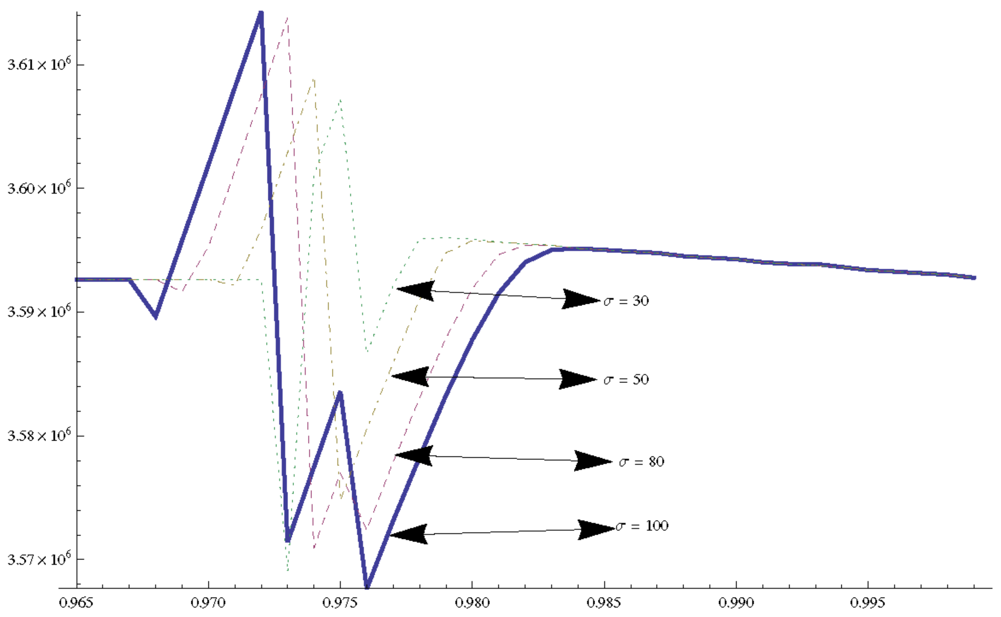
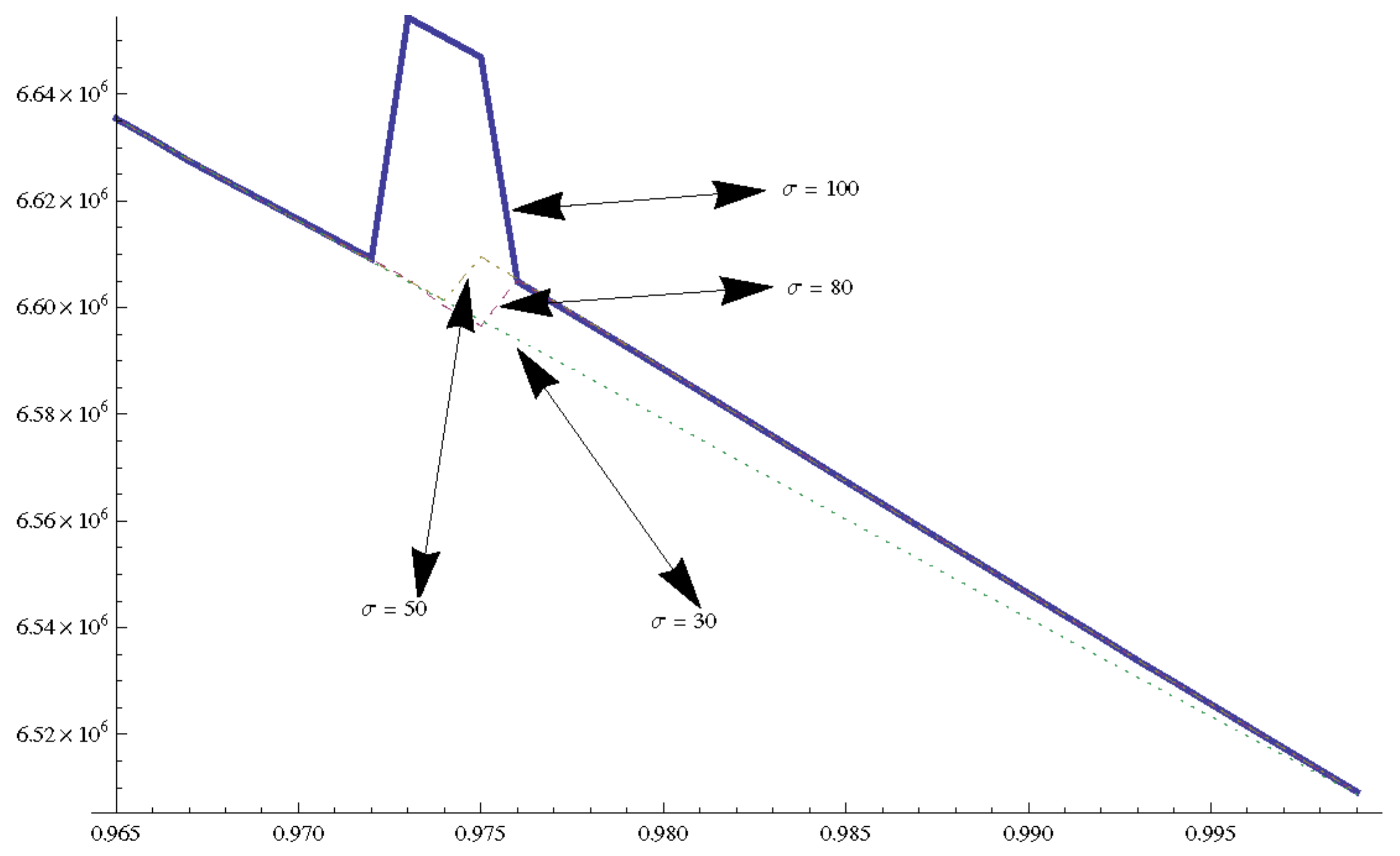
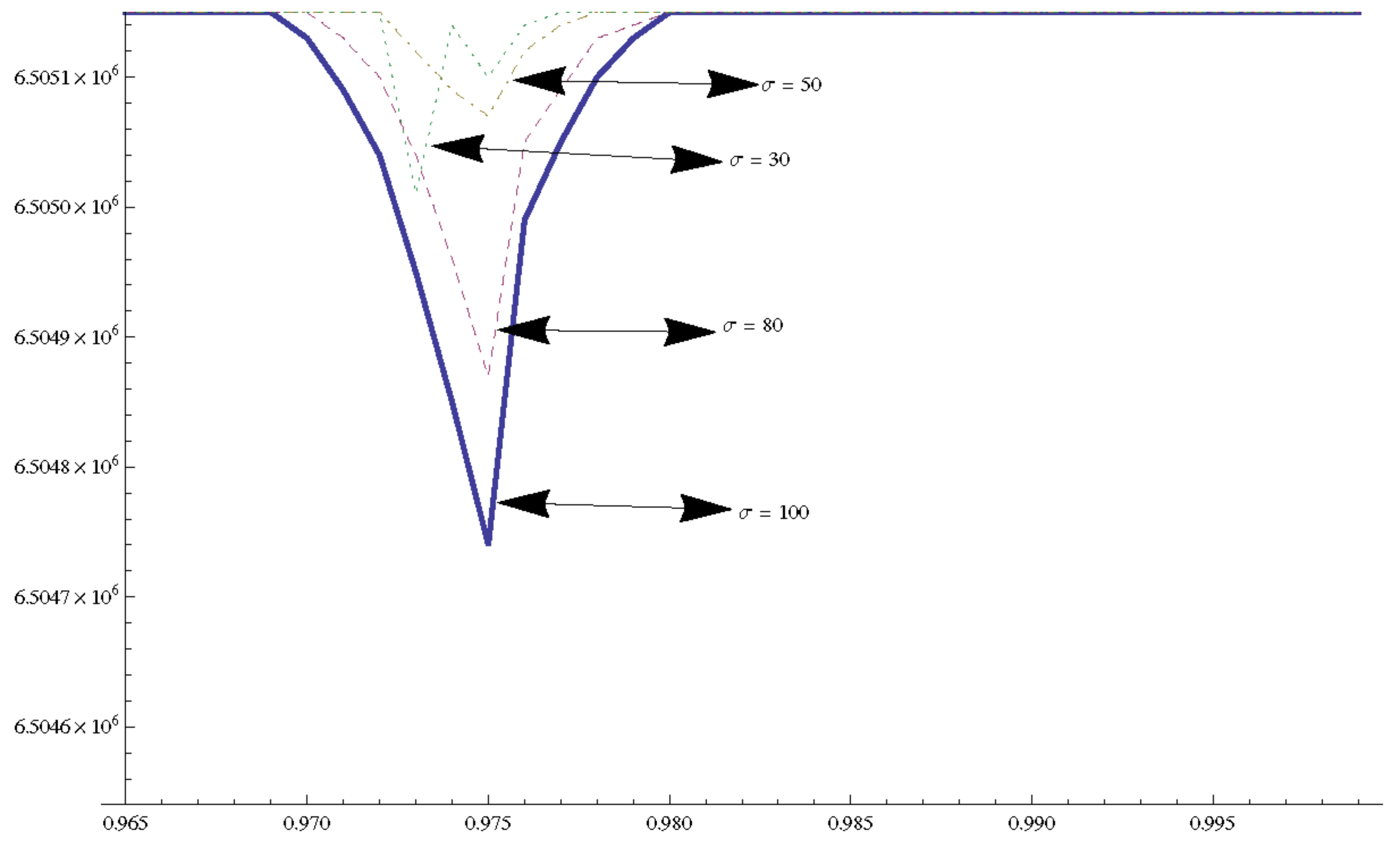
Similarly, the expected revenue of the retailer in Figure 2, the expected revenue of the supplier in Figure 3, and the expected revenue of the supply chain in Figure 4 all have corresponding changes in the corresponding intervals. Figure 1, Figure 2, Figure 3 and Figure 4 show that in the bifurcation mutation interval when $\sigma$ is larger, the optimal order quantity, retailer’s expected revenue, supplier’s expected revenue, and the entire supply chain’s expected revenue will oscillate in a wider area, and the above-mentioned factors will oscillate up and down. On the other hand, Figure 5 shows that the revised ‘Profit-CVaR’ chart shows no significant oscillations, indicating that the revised ‘Profit-CVaR’ is more stable as a risk measure criterion.

5. Conclusions

Under the premise of random market prices, an emergency quantity discount contract model of retailer’s risk neutrality and supplier’s risk aversion is constructed. This paper revises the existing risk measurement criteria, studies the coordination problem of the supply chain under the new risk measurement, and analyzes a numerical example. The following conclusions can be drawn after the analysis.

In the case of market price randomness and supplier risk aversion, the bifurcation and mutation phenomenon appears when the quantity discount contract is used to coordinate the supply chain. Supply chain coordination cannot be achieved in the region of bifurcation mutation, while supply chain coordination can be achieved outside the region of bifurcation mutation. Therefore, it can be seen that when suppliers are averse to risk, the managers in the supply chain should try to avoid the phenomenon of bifurcation and mutation in the supply chain; in other words: avoid cooperation in the bifurcation and sudden change areas. Otherwise, the supply chain members will not be able to maximize their benefits at the same time.

When the decision-maker encounters a risk for the first time, the risk decision-maker may have an ‘allergic reaction’, that is, the decision-maker will be overly nervous and even at a loss when facing a small risk. When the risk is large to a certain extent, or the decision-maker realizes that the risk is very likely to occur, on the contrary, he will not be particularly sensitive to the risk. The above phenomenon is consistent with objective reality. For example, when the decision-maker has no experience in handling risks at the beginning of preventing risks, he is abnormally uncomfortable with the first coming of risks, and various decision-making errors will often occur. On the other hand, when the decision-makers have experienced risks, or when the risks must occur, they will calmly respond instead. This kind of irrational phenomenon at the beginning of the defence risk can be regarded as a normal objective phenomenon, and managers should treat it correctly.

When a quantity discount contract is used to coordinate a supply chain with random prices and supplier risk aversion, the relevant elements of the supply chain will undergo bifurcation and mutation. The larger the standard deviation of the market demand distribution function, the larger the bifurcation mutation area of each element in the supply chain. The upper and lower amplitude of each element will increase accordingly. However, the maximum order quantity that appears in the bifurcation region does not correspond to the maximum expected return of the supply chain. There is a phenomenon of diseconomies of scale. This shows that risk decision-makers should try to prevent the occurrence of bifurcation and mutation when making centralized decisions in management practice. When risks are about to arise, and the situation is unclear, do not decide to cooperate lightly and wait until the situation is clear before making a decision.

The research of this paper is based on the premise of complete information symmetrical. Therefore, it only considers the coordination problem of the secondary supply chain with supplier risk aversion and retailer risk-neutral under the condition of random price. On this basis, we can further study supply chain coordination in the case of information asymmetry and risk aversion at the same time between supply and sales parties.

References

1. Monahan, J.P. A quantity discount pricing model to increase vendor profits. Manag. Sci. 1984, 30, 720–726. [Google Scholar] [CrossRef]
2. Cachon, G.P. Supply Chain coordination with contracts. Handb. Oper. Res. Manag. Sci. 2003, 11, 227–339. [Google Scholar]
3. Huang, X.; Choi, S.-M.; Ching, W.-K.; Siu, T.-K.; Huang, M. On supply chain coordination for false failure returns: A quantity discount contract approach. Int. J. Prod. Econ. 2011, 133, 634–644. [Google Scholar] [CrossRef]
4. Sun, Y.; Xu, X.; Hua, Z. Mitigating bankruptcy propagation through contractual incentive schemes. Decis. Support Syst. 2012, 53, 634–645. [Google Scholar] [CrossRef]
5. Ogier, M.; Cung, V.; Boissiere, J.; Chung, S.H. Decentralised planning coordination with quantity discount contract in a divergent supply chain. Int. J. Prod. Res. 2013, 51, 2776–2789. [Google Scholar] [CrossRef]
6. Kwong, C.K.; Xia, Y.; Chan, C.Y.; Lp, W.H. Incorporating contracts with retailer into product line extension using Stackelberg game and nested bi-level genetic algorithms. Comput. Ind. Eng. 2021, 151, 106976. [Google Scholar] [CrossRef]
7. Yu, D.; Yang, H.; Wu, J. Electricity Supply Chain Coordination Based on Quantity DISCOUNT CONtracts. In Proceedings of the IEEE International Conference on Industrial Technology, Churchill, Australia, 10–13 February 2009; IEEE: Piscataway, NJ, USA, 2009. [Google Scholar]
8. Sheen, G.J.; Tsao, Y.C. Channel coordination, trade credit and quantity discounts for freight cost. Transp. Res. Part E Logist. Transp. Rev. 2007, 43, 112–128. [Google Scholar] [CrossRef]
9. Wang, Z.; Liu, S. Supply Chain Coordination under Trade Credit and Quantity Discount with Sales Effort Effects. Math. Probl. Eng. 2018, 2018, 2190236. [Google Scholar] [CrossRef] [Green Version]
10. Zhang, Q.; Dong, M.; Luo, J.; Segerstedt, A. Supply chain coordination with trade credit and quantity discount incorporating default risk. Int. J. Prod. Econ. 2014, 153, 352–360. [Google Scholar] [CrossRef]
11. Zhou, Y.; Kim, K. Optimal concession contract between a port authority and container-terminal operators by revenue-sharing schemes with quantity discount. Marit. Policy Manag. 2019. [Google Scholar] [CrossRef]
12. Zhang, Y.; Yang, X.; Zhang, W.; Chen, W. Online ordering rules for the multi-period newsvendor problem with quantity discounts. Ann. Oper. Res. 2020, 288, 495–524. [Google Scholar] [CrossRef]
13. Peng, H.; Zhou, M. Quantity Discount Supply Chain Models with Fashion Products and Uncertain Yields. Math. Probl. Eng. 2013, 2013, 895784. [Google Scholar] [CrossRef]
14. Zhao, T.; Xu, X.; Chen, Y.; Liang, L.; Yu, Y.; Wang, K. Coordination of a fashion supply chain with demand disruptions. Transp. Res. Part E Logist. Transp. Rev. 2020, 134, 101838. [Google Scholar] [CrossRef]
15. Lee, J.-Y. Quantity discounts based on the previous order in a two-period inventory model with demand uncertainty. J. Oper. Res. Soc. 2008, 59, 1004–1011. [Google Scholar] [CrossRef]
16. Nie, T.; Du, S. Dual-fairness Supply Chain with Quantity Discount Contracts. Eur. J. Oper. Res. 2017, 258, 491–500. [Google Scholar] [CrossRef]
17. Huang, Y.S.; Ho, R.S.; Fang, C.C. Quantity discount coordination for allocation of purchase orders in supply chains with multiple suppliers. Int. J. Prod. Res. 2015, 53, 6653–6671. [Google Scholar] [CrossRef]
18. Zhang, Q.; Luo, J.; Duan, Y. Buyer–vendor coordination for fixed lifetime product with quantity discount under finite production rate. Int. J. Syst. Sci. 2016, 47, 821–834. [Google Scholar] [CrossRef]
19. Zheng, Q.; Zhou, L.; Fan, T.; Ieromonachou, P. Joint procurement and pricing of fresh produce for multiple retailers with a quantity discount contract. Transp. Res. Part E Logist. Transp. Rev. 2019, 130, 16–36. [Google Scholar] [CrossRef]
20. Agrawal, V.; Seshadri, S. Risk intermediation in supply chain. IIE Trans. 2000, 32, 819–831. [Google Scholar] [CrossRef] [Green Version]
21. Liang, D.; Li, G.; Sun, L. The Effect of Risk Aversion on Manufacturer Advertising in a Two-Stage Supply Chain. Transp. J. 2012, 51, 59–79. [Google Scholar] [CrossRef]
22. Bai, X.; Liu, Y. Robust optimization of supply chain network design in fuzzy decision system. J. Intell. Manuf. 2016, 27, 1131–1149. [Google Scholar] [CrossRef]
23. Rockafller, T.R.; Uryasev, S. Optimization of conditional value-at-risk. J. Risk 2000, 2, 21–24. [Google Scholar] [CrossRef] [Green Version]
24. Rockafller, T.R.; Uryasev, S. Conditional value-at-risk for general loss distribution. J. Bank. Financ. 2002, 26, 1443–1471. [Google Scholar] [CrossRef]
25. Tao, L.; Liu, S.; Xie, N.; Javed, S.A. Optimal position of supply chain delivery window with risk-averse suppliers: A CVaR optimization approach. Int. J. Prod. Econ. 2021, 232, 107989. [Google Scholar] [CrossRef]
26. Chen, Z.; Yuan, K.; Zhou, S. Supply chain coordination with trade credit under the CVaR criterion. Int. J. Prod. Res. 2019, 57, 3538–3553. [Google Scholar] [CrossRef]
Figure 1. The bifurcation figure of optimal order quantity.
Mathematics 09 01791 g001
Figure 2. The bifurcation figure of retailer’s expected profits.
Mathematics 09 01791 g002
Figure 3. The bifurcation figure of the supplier’s expected profits.
Mathematics 09 01791 g003
Figure 4. The bifurcation figure of the supply chain’s expected profits.
Mathematics 09 01791 g004
Figure 5. The trend figure of “ π s + C V a R ( π r ) ”.
Mathematics 09 01791 g005