A New Class of Plane Curves with Arc Length Parametrization and Its Application to Linear Analysis of Curved Beams

Abstract

The objective of this paper is to define one class of plane curves with arc-length parametrization. To accomplish this, we constructed a novel class of special polynomials and special functions. These functions form a basis of $L^2\left(\mathbb{R}\right)$ space and some of their interesting properties are discussed. The developed curves are used for the linear static analysis of curved Bernoulli–Euler beam. Due to the parametrization with arc length, the exact analytical solution can be obtained. These closed-form solutions serve as the benchmark results for the development of numerical procedures. One such example is provided in this paper.

1. Introduction

Arc-length parametrization can be considered to be the most natural of all possible parametrizations of a given curve [1]. This parametrization is very useful and has several useful mathematical properties. Unfortunately, there is a limited set of curves for which the arc-length parametrization can be expressed as an elementary function. It is proved in [2] that, on par with polynomials, it is possible to select a subclass of arc-length curves that has an arbitrary number of degrees of freedom.

These curves are useful in engineering applications, especially for the analysis of beam-like structures. If induced beam theories are employed for the analysis of these systems, a three-dimensional beam continuum is reduced to an arbitrary curved line [3]. Under specific kinematic restrictions, a classical mechanical model of a planar curved Bernoulli–Euler beam emerges. The linear static equations of this beam model are considered in reference [4] with respect to an arbitrary parametric coordinate.

The beam equations rarely have an analytical solution. Therefore, it is of a particular interest to examine arc-length curves for which the governing equations of Bernoulli–Euler beam are significantly simplified, and analytical solutions are feasible. These solutions can provide valuable benchmark test results for the application of modern numerical methods to the analysis of free-form beams [5,6].

Special polynomials and functions are the subject of many books and papers and have many applications [7,8], especially in physics where they are used for solving differential equations [9]. The two main objectives of this paper are: (i) construction of one class of plane curves that has arc-length parametrization (Section 3 and Section 4), and (ii) application of the introduced curves in computational mechanics and numerical analysis (Section 5). In Section 3 special functions, $f_n$, $n\in {\mathbb{N}}_0$, are constructed using polynomials $F_n$, $n\in {\mathbb{N}}_0$, which are called special polynomials. It is proved that special polynomials $F_0=1$, $F_n$, $n\in \mathbb{N}$, are solutions of the Sturm–Liouville differential equation [10]

$$(x^2+1)y^{″}\left(x\right)-2(2n-1)x{y}^{\prime }\left(x\right)+2n(2n-1)y\left(x\right)=0,$$

(1)

while special functions $f_0=1$, $f_n$, $n\in \mathbb{N}$, are solutions of the Sturm–Liouville differential equation [11]

$${(x^2+1)}^2{y}^{″}\left(x\right)+2x(x^2+1)y^{\prime }\left(x\right)+4n^{2}y\left(x\right)=0$$

(2)

and they form the basis of an $L^2\left(\mathbb{R}\right)$ space [12], with respect to the weight function $\omega \left(x\right)=\frac{1}{1+x^2}$. In Section 4, using the special functions $f_n,n\in {\mathbb{N}}_0$, plane curves with arc-length parametrization are constructed and some features of these curves are proved. Linear static analysis of one planar curved beam is reported in Section 5.

2. Preliminaries

We employ the following notation: $\mathbb{N}$, $\mathbb{R}$, ${\mathbb{R}}^{+}$ and $\mathbb{C}$ for the sets of positive integers, real, positive real and complex numbers, respectively. Additionally, ${\mathbb{N}}_0=\mathbb{N}\cup \left\{0\right\}$. For a given complex number z, we denote with $\Re \left(z\right)$ the real, and with $\Im \left(z\right)$ the imaginary, part. The Taylor series of $y=f\left(x\right)$ at the point $x_0$ is $f\left(x\right)={\sum }_{k=0}^n\frac{f^{\left(k\right)}\left(x_0\right)}{k!}{(x-x_0)}^k+R_{n+1}\left(x\right),$ where $R_{n+1}\left(x\right)$ is a residual. By $L^2\left(\mathbb{R}\right)$ we denote the space of a square integrable functions. We also use a polylogarithm special function of order 2 (called the dilogarithm) defined by $PolyLog(2,z)={\sum }_{n=1}^{\infty }\frac{z^n}{n^2}$, $z\in \mathbb{C}$, [13].

Arc-Length Parametrization of Plane Curves

The arc length of a differentiable curve $\mathbf{r}\left(s\right)=⟨x\left(s\right),y\left(s\right)⟩$ from the point $s=0$ is given by

$$l\left(s\right)={\int }_0^s\left|{\mathbf{r}}^{\prime }\left(t\right)\right|dt={\int }_0^s\sqrt{x^{\prime 2}\left(t\right)+y^{\prime 2}\left(t\right)}dt.$$

(3)

To calculate arc-length parametrization, the inverse function $l^{-1}$ must be well-defined and monotonically increasing. A necessary and sufficient condition for a curve to have the arc-length parametrization form is that for all s,

$$l\left(s\right)=s.$$

(4)

If we take the derivative with respect to s in (4) and substitute it in (3), another necessary and sufficient condition for the arc-length parametrization is obtained

$$x^{\prime 2}\left(s\right)+y^{\prime 2}\left(s\right)=1.$$

(5)

Equation (5) is equivalent to the condition that the hodograph lies on the unit circle centered at the origin

$$|{\mathbf{r}}^{\prime }\left(s\right)|=1,$$

(6)

so that the curvature of the curve at each point is given by

$$\kappa \left(s\right)=|{\mathbf{r}}^{″}\left(s\right)|.$$

(7)

3. Special Polynomials and Special Functions

The special polynomials $F_n\left(x\right),n\in \mathbb{N}$, introduced in [10,14], are defined by:

$$\begin{array}{cc}\hfill F_0\left(x\right)=1,F_{2n}\left(x\right)& {\displaystyle =\Re \left({(x-i)}^{2n}\right)=\sum _{k=0}^n{(-1)}^{n+k}\left(\genfrac{}{}{0pt}{}{2n}{2k}\right)x^{2k}}\hfill \\ \hfill F_{2n-1}\left(x\right)& {\displaystyle =\Im \left({(x-i)}^{2n}\right)=\sum _{k=1}^n{(-1)}^{n+k+1}\left(\genfrac{}{}{0pt}{}{2n}{2k-1}\right)x^{2k-1}}\hfill \end{array}$$

(8)

Following [10], several properties of the special polynomials are obtained.

Proposition 1.

Polynomials $F_{2n-1}\left(x\right)$ and $F_{2n}\left(x\right)$, $n\in \mathbb{N}$, satisfy:

$$F_{2n}\left(x\right)=\frac{x^2+1}{2n}{F}_{2n-1}^{\prime }\left(x\right)-x{F}_{2n-1}\left(x\right)$$

(9)

and

$$F_{2n-1}\left(x\right)=-\frac{x^2+1}{2n}{F}_{2n}^{\prime }\left(x\right)+x{F}_{2n}\left(x\right).$$

(10)

Proof. 

Notice that

$$F_{2n}\left(x\right)+i{F}_{2n-1}\left(x\right)={(x-i)}^{2n},$$

(11)

from which it follows

$$F_{2n}^{\prime }\left(x\right)+i{F}_{2n-1}^{\prime }\left(x\right)=2n{(x-i)}^{2n-1}.$$

(12)

By multiplying (12) with $x-i$ and taking the real and imaginary parts we obtain the system

$$\genfrac{}{}{0pt}{}{x{F}_{2n}^{\prime }\left(x\right)+F_{2n-1}^{\prime }\left(x\right)=2n{F}_{2n}\left(x\right)}{-F_{2n}^{\prime }\left(x\right)+x{F}_{2n-1}^{\prime }\left(x\right)=2n{F}_{2n-1}\left(x\right)}$$

(13)

from which (9) and (10) follow. □

Corollary 1.

For $F_{2n-1}\left(x\right)$ and $F_{2n}\left(x\right)$, $n\in \mathbb{N}$, the following holds

$$F_{2n-1}^2\left(x\right)+F_{2n}^2\left(x\right)={(x^2+1)}^{2n}.$$

(14)

Theorem 1.

Polynomials $F_n\left(x\right)$, $n\in {\mathbb{N}}_0$, are solutions of the Sturm–Liouville differential Equation (1). Moreover, $y_n\left(x\right)=C_1{F}_{2n-1}\left(x\right)+C_2{F}_{2n}\left(x\right)$ are the only solutions of (1).

Proof. 

We will prove the assertion only for polynomials $F_{2n-1}\left(x\right)$, since the proof for polynomials $F_{2n}\left(x\right)$, $n\in \mathbb{N}$, is the same. The derivation of (9) yields

$$(x^2+1)F_{2n-1}^{″}\left(x\right)-2(n-1)x{F}_{2n-1}^{\prime }\left(x\right)-2n{F}_{2n-1}\left(x\right)=2n{F}_{2n}^{\prime }\left(x\right).$$

(15)

From (13) we obtain

$$(x^2+1)F_{2n-1}^{″}\left(x\right)-2(2n-1)x{F}_{2n-1}^{\prime }\left(x\right)+2n(2n-1)F_{2n-1}\left(x\right)=0.$$

(16)

Conversely, we know that $y_1\left(x\right)=F_{2n-1}\left(x\right)$ is the particular solution of (1). The general solution is of the form $y\left(x\right)=C_1{y}_1\left(x\right)+C_2{y}_2\left(x\right)$, where

$$y_2\left(x\right)=F_{2n-1}\left(x\right)\int \frac{{(x^2+1)}^{2n-1}}{F_{2n-1}^2\left(x\right)}dx.$$

(17)

On the other hand, using (14) we obtain

$${\left(\frac{F_{2n}\left(x\right)}{F_{2n-1}\left(x\right)}\right)}^{\prime }=2n\frac{{(x^2+1)}^{2n-1}}{F_{2n-1}^2\left(x\right)}$$

(18)

from which it follows

$$y_2\left(x\right)=\frac{F_{2n}\left(x\right)}{2n}.$$

(19)

Therefore, $y\left(x\right)=C_1{F}_{2n-1}\left(x\right)+C_2{F}_{2n}\left(x\right)$. □

Using polynomials $F_n\left(x\right)$, $n\in \mathbb{N}$, we define special functions as follows:

$$f_0\left(x\right)=1,f_{2n-1}\left(x\right)={(-1)}^{n-1}\frac{F_{2n-1}\left(x\right)}{{(x^2+1)}^n},f_{2n}\left(x\right)={(-1)}^n\frac{F_{2n}\left(x\right)}{{(x^2+1)}^n},n\in \mathbb{N}.$$

(20)

Notice that

$$f_{2n-1}\left(x\right)=sin(2narctan\left(x\right)),f_{2n}\left(x\right)=cos(2narctan\left(x\right)),n\in \mathbb{N}.$$

(21)

Theorem 2.

Functions $f_n\left(x\right)$, $n\in {\mathbb{N}}_0$, are solutions of the Sturm–Liouville differential Equation (2). Moreover, $y_n\left(x\right)=C_1{f}_{2n-1}\left(x\right)+C_2{f}_{2n}\left(x\right)$ are the only solutions of (2).

Proof. 

We will prove the assertion only for functions $f_{2n}\left(x\right)$, since the proof for functions $f_{2n-1}\left(x\right)$, $n\in \mathbb{N}$, is the same. The derivation of (21) yields

$$(x^2+1)f_{2n-1}^{\prime }\left(x\right)-2n{f}_{2n}\left(x\right)=0$$

(22)

and

$$(x^2+1)f_{2n}^{\prime }\left(x\right)+2n{f}_{2n-1}\left(x\right)=0.$$

(23)

By calculating the derivation of (23) we obtain

$${(x^2+1)}^2{f}_{2n}^{″}\left(x\right)+2x(x^2+1)f_{2n}^{\prime }\left(x\right)+2n(x^2+1)f_{2n-1}^{\prime }\left(x\right)=0,$$

(24)

so (22) gives assertion. For the converse part we use the same techniques as in Theorem 1. □

Theorem 3.

The set ${\left\{\frac{1}{\sqrt{\pi }}{f}_0\left(x\right),\sqrt{\frac{2}{\pi }}{f}_{2n-1}\left(x\right),\sqrt{\frac{2}{\pi }}{f}_{2n}\left(x\right)\right\}}_{n=1}^{\infty }$ is an orthonormal basis in $L^2\left(\mathbb{R}\right)$ with respect to the weight function

$$\omega \left(x\right)=\frac{1}{1+x^2}.$$

(25)

Proof. 

The proof follows from ([10], Theorem 5.2) (see also Lemma 3.11, Theorem 3.12 and Corollary 3.13 in [10]). □

4. Arc-Length Parametrization Using Special Functions

In this section, plane curves with arc-length parametrization are constructed using the new class of special functions $f_n,n\in {\mathbb{N}}_0$. We consider a smooth curve of the form

$$r_a^{\prime }\left(s\right)=⟨C_a\left(s\right),S_a\left(s\right)⟩,a\in {\mathbb{R}}^{+},s\in \mathbb{R},$$

(26)

where $C_a\left(s\right)=cos(aarctan\left(s\right))$, $S_a\left(s\right)=sin(aarctan\left(s\right))$. For $a=2n$

$${\mathbf{r}}_{2n}^{\prime }\left(s\right)=⟨f_{2n}\left(s\right),f_{2n-1}\left(s\right)⟩,n\in \mathbb{N},s\in \mathbb{R}.$$

(27)

The necessary and sufficient condition for the arc-length parametrization form in this case is guaranteed by ${cos}^2\left(\alpha \right)+{sin}^2\left(\alpha \right)=1$, $\alpha \in \mathbb{R}$. Arc-length parametrized curves can be constructed by integration, i.e.,

$${\mathbf{r}}_a\left(s\right)=⟨\underset{0}{\overset{s}{\int }}{C}_a\left(t\right)dt,\underset{0}{\overset{s}{\int }}{S}_a\left(t\right)dt⟩,a\in {\mathbb{R}}^{+},s\in \mathbb{R}.$$

(28)

For $a=2n$, functions $f_{2n}\left(s\right)$ and $f_{2n-1}\left(s\right)$, $n\in \mathbb{N}$, are rational. Therefore, it is easy to show, using the standard procedure of integral calculus, that these integrals are elementary functions. Additionally, for $a=n$ integrals in (28) are elementary functions. The curvature of the curve (28) is determined by

$$\kappa \left(s\right)=|{\mathbf{r}}_a^{″}\left(s\right)|=\frac{a}{1+s^2},$$

(29)

and the radius of the curvature is

$$R=\frac{1}{a}(s^2+1).$$

(30)

Since integrals in (28) can be calculated analytically when $a=n$, $n\in \mathbb{N}$, these cases are particularly interesting.

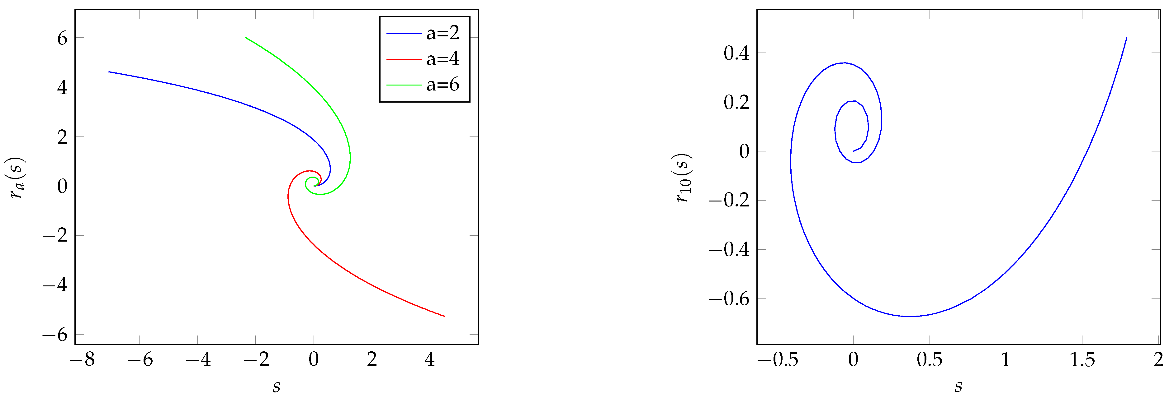
Example 1.

For $a=1$ the curve

$$r_1\left(s\right)=⟨arcsinh\left(s\right),\sqrt{s^2+1}-1⟩.$$

(31)

is assigned to the function

$$y\left(x\right)=coshx-1,x\in \mathbb{R}.$$

(32)

Figure 1 shows curves ${\mathbf{r}}_2\left(s\right),{\mathbf{r}}_4\left(s\right),{\mathbf{r}}_6\left(s\right)$ and ${\mathbf{r}}_{10}\left(s\right)$, $s\in \mathbb{R}$.

Figure 1. Obtained arc-length curves ${\mathbf{r}}_a$ when $a=2$, $a=4$, $a=6$ (left) and $a=10$ (right).

Proposition 2.

For $s\in \left[tan\left(\frac{(2n-1)\pi }{2a}\right),tan\left(\frac{(2n+1)\pi }{2a}\right)\right]$, $2n+1<2a$, $n\in \mathbb{N}$, $a\in {\mathbb{R}}^{+}$, the curve (28) can be represented as a function $y=y\left(x\right)$ which reaches extreme values for $s_e=tan\left(\frac{n\pi }{a}\right)$.

Proof. 

The direction of the tangent of the curve represented by (28) is

$$y_x^{\prime }\left(s\right)=tan(aarctan\left(s\right)).$$

(33)

This direction is defined if $x^{\prime }\left(s\right)=cos(aarctan\left(s\right))\ne 0$, i.e., $s\ne tan\left(\frac{(2n+1)\pi }{2a}\right)$, $2n+1<2a$, $n\in \mathbb{N},a\in {\mathbb{R}}^{+}$. The stationary points can be calculated from

$$y_x^{\prime }\left(s\right)=tan(aarctan\left(s\right))=0\Rightarrow sin(aarctan\left(s\right))=0,$$

(34)

so we have $s_e=tan\left(\frac{n\pi }{a}\right)$. One can easily prove that these stationary points are extreme values of the function $y=y\left(x\right)$. □

Remark 1.

Notice that extreme values $s_e=tan\left(\frac{n\pi }{2n}\right)$ are zeros of the polynomials $F_{2n}\left(x\right)$, $n\in \mathbb{N}$.

From Proposition 2 it holds that $s=tan\left(\frac{n\pi }{a}\right)$, $2n<a$, $n\in \mathbb{N}$, $a\in {\mathbb{R}}^{+}$, are solutions of the following equation

$$tan(aarctan(s\left)\right)=0.$$

(35)

This means that for $s=tan\left(\frac{n\pi }{a}\right)$, $2n<a$, $n\in \mathbb{N}$, $a\in {\mathbb{R}}^{+}$, the tangent of the curve (28) is parallel to the $O_x$ axis.

Proposition 3.

The Taylor series of the curve (28) considered as a function $y=y\left(x\right)$ in a neighborhood of its extreme value $s_e$ is

$$y\left(x\right)=y\left(s_e\right)+\frac{a}{1+s_e^2}{(x-x\left(s_e\right))}^2+\dots .$$

(36)

Proof. 

Using formula:

$$\begin{array}{cc}\hfill y_x^{\prime }\left(s\right)=\frac{y^{\prime }\left(s\right)}{x^{\prime }\left(s\right)},y_x^{{}^{″}}\left(s\right)& =\frac{\frac{d}{ds}\left(y_x^{\prime }\left(s\right)\right)}{x^{\prime }\left(s\right)}=\frac{y^{″}\left(s\right)x^{\prime }\left(s\right)-x^{″}\left(s\right)y^{\prime }\left(s\right)}{{\left(x^{\prime }\left(s\right)\right)}^3},\dots \hfill \\ \hfill y_x^{\left(n\right)}\left(s\right)& =\frac{\frac{d}{ds}\left(y_x^{(n-1)}\left(s\right)\right)}{x^{\prime }\left(s\right)},n>2.\hfill \end{array}$$

(37)

we obtain the required result. □

Remark 2.

Notice that the curve (28) has the Taylor series in a neighborhood of an arbitrary point $s_0\in \left(tan\left(\frac{(2n-1)\pi }{2a}\right),tan\left(\frac{(2n+1)\pi }{2a}\right)\right)$. For the sake of simplicity, let us consider only the case when $s_0=s_e$, since the Taylor series is then even function.

Example 2.

If $s_0=0$, the curve (28) can be expanded into a Maclaurin series of the form

$$\genfrac{}{}{0pt}{}{y\left(x\right)=a{x}^2+(3a^4-2a^2)x^4+(24a-68a^3+45a^5)x^6}{+(-720a+2928a^3-3782a^5+1575a^7)x^8+\dots }$$

(38)

5. An Application to the Linear Static Analysis of Curved Beams

Let us consider one application of the arc-length parametrized curves we have introduced. In this example, we deal with the linear static analysis of curved beams, as discussed in [4]. For a general 3D case and an arbitrary parametric coordinate, beam equations are the set of four linear first order differential equations:

• force equations: $F_{k|1}=f_k^F(f_k^F=\sqrt{g}{p}_k)$;
• moment equations: $M_{k|1}=f_k^M\left(f_k^M=\sqrt{g}(m_k-e_{1mk}{F}^m)\right)$;
• rotation equations: ${\phi }_{k|1}=f_k^{\phi }\left(f_1^{\phi }=\sqrt{g}{\kappa }_1,f_j^{\phi }=({\kappa }_j-K_j{\epsilon }_{11})/\sqrt{g},j=2,3\right)$;
• displacement equations: $u_{k|1}=f_k^u(f_1^u={\epsilon }_{11},f_2^u=\sqrt{g}{\phi }_3,f_3^u=-\sqrt{g}{\phi }_2)$,

where ${(•)}_{k|1}$ is the covariant derivative of a kth component of a vector with respect to the parametric coordinate $\xi$; $F_k,M_k,{\phi }_k$ and $u_k$ are the components of the section force, section couple, infinitesimal rotation, and displacement, respectively; g is the component of the metric tensor which is equal to its determinant; $p_k$ and $m_k$ are the components of distributed load and moment, respectively; ${\kappa }_j$ are the curvature changes, while $K_j$ are the initial curvatures of beam axis; ${\epsilon }_{11}$ is the axial strain of beam axis while $e_{ijk}$ is the permutation symbol.

It is shown in [4] that the solutions of the beam equations are:

$$\begin{array}{cc}\hfill F_k\left(\xi \right)& =x_{,k}^n\left(\xi \right)\left(F_n^{*}\left({\xi }_i\right)+{\int }_{{\xi }_i}^{\xi }{f}_m^F\left(t\right)x_n^{,m}\left(t\right)dt\right),\hfill \end{array}$$

(39)

$$\begin{array}{cc}\hfill M_k\left(\xi \right)& =x_{,k}^n\left(\xi \right)\left(M_n^{*}\left({\xi }_i\right)+{\int }_{{\xi }_i}^{\xi }{f}_m^M\left(t\right)x_n^{,m}\left(t\right)dt\right),\hfill \end{array}$$

(40)

$$\begin{array}{cc}\hfill {\phi }_k\left(\xi \right)& =x_{,k}^n\left(\xi \right)\left({\phi }_n^{*}\left({\xi }_i\right)+{\int }_{{\xi }_i}^{\xi }{f}_m^{\phi }\left(t\right)x_n^{,m}\left(t\right)dt\right),\hfill \end{array}$$

(41)

$$\begin{array}{cc}\hfill u_k\left(\xi \right)& =x_{,k}^n\left(\xi \right)\left(u_n^{*}\left({\xi }_i\right)+{\int }_{{\xi }_i}^{\xi }{f}_m^u\left(t\right)x_n^{,m}\left(t\right)dt\right),\hfill \end{array}$$

(42)

where $x_{,k}^n$ and $x_n^{,k}$ are the components of the base and reciprocal base vectors of the beam axis, respectively. ${\xi }_i$ represents a coordinate of some fixed beam section, while an asterisk denotes quantities measured with respect to the global Cartesian coordinate system. That is, ${(•)}_1^{*}={(•)}_x,{(•)}_2^{*}={(•)}_y,{(•)}_3^{*}={(•)}_z$. Standard summation convention is applied, and indices take values of 1, 2, and 3.

These equations have an analytical solution in only a few, special cases, primarily due to the fact that the square of the determinant of the metric tensor, which equals Jacobian, is a function. Arc-length parametrization simplifies these equations significantly since $g=1$, and the basis and its dual counterpart become the same. Furthermore, for the in-plane beam the following is valid: $F_3=M_1=M_2={\phi }_1={\phi }_2=u_3=p_3=m_1=m_2=0$, and $M_3=M,m_3=m,K_3=K,{\kappa }_3=\kappa$, and ${\phi }_3=\phi$.

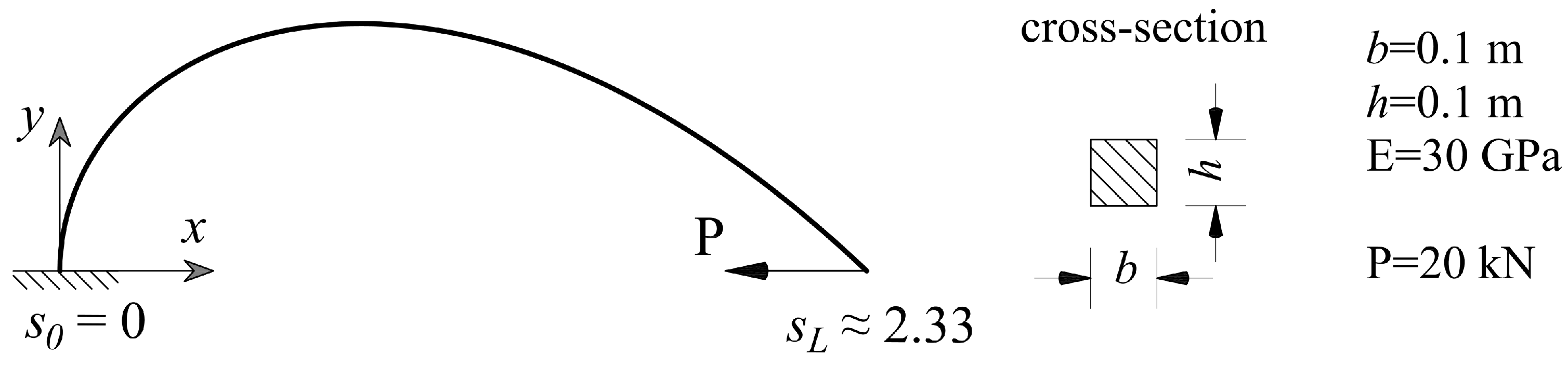
Let us consider a beam as in Figure 2. The beam axis is described with:

$$x\left(s\right)=ln(1+s^2),y\left(s\right)=2arctan\left(s\right)-s,s\in [0,s_L],$$

(43)

where $s_L$ is the solution of the equation $y\left(s_L\right)=0$ ($s_L\approx 2.331122370414423$). The other geometric and material characteristics of the beam are displayed in Figure 2. To simplify the example, the beam is clamped at one, $s=0$, and free at the other, $s=s_L$, end. This results with the homogeneous kinematic boundary conditions for $s=0$, i.e.: $\phi \left(0\right)=u_1\left(0\right)=u_2\left(0\right)=0$. Furthermore, the beam is statically determinate, and the force boundary conditions are simply calculated as: $F_2^{*}\left(0\right)=M\left(0\right)=0,F_1^{*}\left(0\right)=20\mathrm{kN}.$

Figure 2. Geometric and material properties, and applied load.

The beam equations for this example reduce to:

$$F_{k,1}=0,M_{,1}=-F_2,{\phi }_{,1}=\kappa ,u_{1,1}={\epsilon }_{11},u_{2,1}=\phi ,$$

(44)

where ${(•)}_{,1}$ is the partial derivative with respect to the arc-length coordinate s. Now, it is straightforward to calculate section forces and section couple, since $p_1=p_2=m=0$. However, rotation and displacement must be calculated by integration.

The base vectors, the tangent and the normal, are:

$$\begin{array}{cc}\hfill \mathbf{t}& ={\mathbf{g}}_1=⟨x_{,1}^1,x_{,1}^2⟩=⟨sin(2arctan\left(s\right)),cos(2arctan\left(s\right))⟩\hfill \\ \hfill \mathbf{n}& ={\mathbf{g}}_2=⟨x_{,2}^1,x_{,2}^2⟩=⟨cos(2arctan\left(s\right)),-sin(2arctan\left(s\right))⟩,\hfill \end{array}$$

(45)

which gives section forces and section couple as:

$$\begin{array}{cc}\hfill F_1\left(s\right)& =x_{,1}^1\left(s\right)F_1^{*}\left(0\right)=-20sin(2arctan\left(s\right))\hfill \\ \hfill F_2\left(s\right)& =x_{,2}^1\left(s\right)F_1^{*}\left(0\right)=-20cos(2arctan\left(s\right)),\hfill \\ \hfill M\left(s\right)& =-{\int }_0^s{F}_2\left(t\right)dt=-20(s-2arctan\left(s\right)).\hfill \end{array}$$

(46)

Using the simplest constitutive relation [4], the axial strain and the curvature change of the beam axis are:

$${\epsilon }_{11}\left(s\right)=\frac{F_1\left(s\right)}{Ebh}=-\frac{sin(2arctan(s\left)\right)}{15,000},\kappa \left(s\right)=\frac{12M}{Eb{h}^3}=-\frac{2(s-2arctan(s\left)\right)}{25}.$$

(47)

When comparing our results with those obtained with the finite element of a straight beam, it is reasonable to exclude the term $K{\epsilon }_{11}$ since it is specific for curved beams. Now, the rotation is calculated as:

$$\phi \left(s\right)={\int }_0^s\kappa \left(t\right)dt=\frac{1}{25}(4sarctan\left(s\right)-2ln(1+s^2)-s^2),$$

(48)

while the global displacement components are:

$$\begin{array}{cc}\hfill u_1^{*}\left(s\right)& ={\int }_0^s({\epsilon }_{11}\left(t\right)x_{,1}^1\left(t\right)+\phi \left(t\right)x_{,2}^1\left(t\right))dt=\frac{1}{15,000}\left(\frac{2s}{1+s^2}-2arctan\left(s\right)\right.\hfill \\ \hfill & +200(-12s+s^3-6arctan\left(s\right)\left(s^2-2+8ln\left(\frac{2}{\sqrt{1+s^2}}\right)\right)\hfill \\ \hfill & +6(s-2arctan\left(s\right))ln(1+s^2)\left.+24\Re \left(iPolyLog\left(2,\frac{s-i}{s+i}\right)\right))\right),\hfill \\ \hfill u_2^{*}\left(s\right)& ={\int }_0^s({\epsilon }_{11}\left(t\right)x_{,1}^2\left(t\right)+\phi \left(t\right)x_{,2}^2\left(t\right))dt=\frac{1}{15,000}\left(\frac{2s^2}{1+s^2}+ln(1+s^2)\right.\hfill \\ & \left.+600\left(s^2+4arctan\left(s\right)·(arctan\left(s\right)-2s)+ln(1+s^2)\left(3+ln(1+s^2)\right)\right)\right),\hfill \end{array}$$

(49)

where ${\displaystyle \Re \left(iPolyLog\left(2,\frac{s-i}{s+i}\right)\right)=\sum _{n=1}^{\infty }\frac{{(-1)}^{n+1}}{n^2}sin(2narctan\left(s\right)).}$

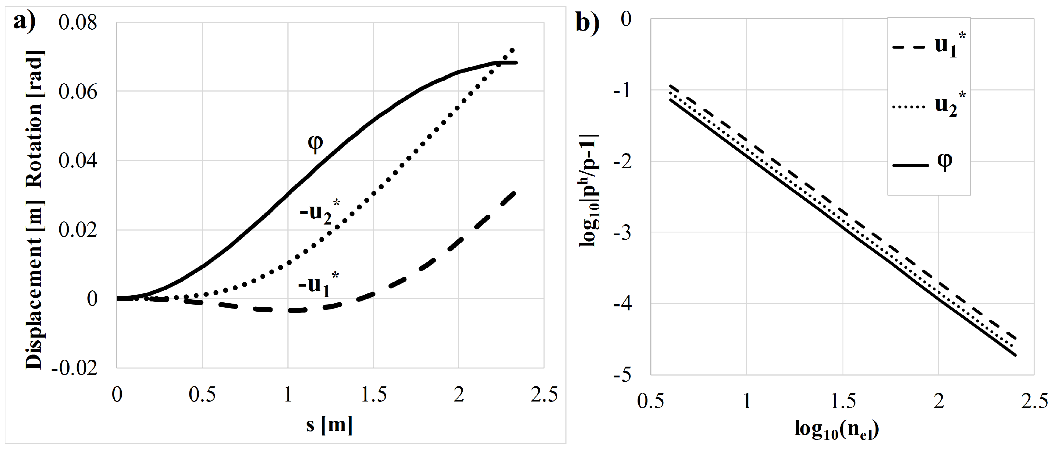
The obtained functions of rotation and displacement are shown in Figure 3a. Furthermore, the beam is analyzed with the standard 2-node finite element which employs cubic Hermite polynomials for transverse, and linear polynomials for axial displacements [15]. Kinematic quantities at the point of force application are calculated with different meshes of these elements and the convergences with respect to the calculated analytical results are shown in Figure 3b. Evidently, highly accurate numerical results for this example require dense meshes of finite elements.

Figure 3. (a) Displacement components and rotation as the functions of arc-length coordinate s. (b) Convergence of results for $u_1^{*}\left(s_L\right)$, $u_2^{*}\left(s_L\right)$, and ${\phi }^{*}\left(s_L\right)$, obtained with the Hermite finite element (${\mathbf{p}}^h$), with respect to the number of elements. The analytical solutions (48) and (49) are used as the reference ones (p).

6. Conclusions

In this paper, we have constructed a novel class of special polynomials and special functions and some of its interesting properties are discussed. The uniqueness of this class lies in the fact that these special polynomials are not orthogonal (the special polynomials most commonly used are orthogonal), but the corresponding class of special functions is orthonormal (with respect to the weight function (25)), which is shown in Theorem 3. Furthermore, the derived special functions are used to obtain one class of plane curves with arc-length parametrization.

The differential equations of equilibrium of an arbitrarily curved BE beam rarely have analytical solutions. However, arc-length parametrized curves, such as the ones introduced here, allow us to find the exact solutions for the linear static analysis of curved beams. The existence of analytical solutions in computational mechanics is highly desirable, since they provide reference benchmark results for the assessment of novel mechanical models and numerical methods.