The Mathematics of Quasi-Diffusion Magnetic Resonance Imaging

Abstract

Quasi-diffusion imaging (QDI) is a novel quantitative diffusion magnetic resonance imaging (dMRI) technique that enables high quality tissue microstructural imaging in a clinically feasible acquisition time. QDI is derived from a special case of the continuous time random walk (CTRW) model of diffusion dynamics and assumes water diffusion is locally Gaussian within tissue microstructure. By assuming a Gaussian scaling relationship between temporal ($\alpha$) and spatial ($\beta$) fractional exponents, the dMRI signal attenuation is expressed according to a diffusion coefficient, $D$ (in mm² s⁻¹), and a fractional exponent, $\alpha$. Here we investigate the mathematical properties of the QDI signal and its interpretation within the quasi-diffusion model. Firstly, the QDI equation is derived and its power law behaviour described. Secondly, we derive a probability distribution of underlying Fickian diffusion coefficients via the inverse Laplace transform. We then describe the functional form of the quasi-diffusion propagator, and apply this to dMRI of the human brain to perform mean apparent propagator imaging. QDI is currently unique in tissue microstructural imaging as it provides a simple form for the inverse Laplace transform and diffusion propagator directly from its representation of the dMRI signal. This study shows the potential of QDI as a promising new model-based dMRI technique with significant scope for further development.

1. Introduction

Quasi-diffusion imaging [1] is a novel diffusion magnetic resonance imaging (dMRI) technique based on a special case of the continuous time random walk (CTRW) diffusion model [2,3,4,5]. The diffusion dynamics are represented by an effective normal diffusion where the mean squared-displacement of the diffusing particles is proportional to time, $\langle x^2\rangle ~t$. This corresponds to the fractional exponents representing the probability density functions of the waiting times between steps, $\alpha$, and the step lengths, $\beta$, having the Gaussian scaling relationship,

$$\frac{2\alpha }{\beta }=1.$$

(1)

Consequently, $\alpha$ and $\beta$ exponents are not independent and both processes are described by related inverse power dependencies for step length ($x^{2\left(\alpha -1\right)}$) and waiting time ($t^{\alpha -1}$).

Diffusion MRI provides a probe of tissue microstructure by application of diffusion encoding gradients that sensitise signals to water diffusion within an image voxel [6,7,8,9,10]. In vivo dMRI voxel sizes are typically on a mm scale, whereas tissue microstructural properties are measured in microns (μm). Hence, the dMRI signal includes components from all cells within a voxel, and contributions from the extra-cellular space. When there is restriction of water diffusion at surface boundaries, the pulsed gradient spin echo (PGSE) Nuclear Magnetic Resonance (NMR) diffusion measurement provides a probe of the length scales of anisotropic microstructures [11].

The observed dMRI signal in tissue is non-Gaussian. This has led to the development of numerous techniques to infer attributes of the diffusion environment and to several theories regarding the origin of the non-Gaussian signal [8,9,12,13]. These theories relate to the effect on diffusion by cell membranes, their internal structures, and the complex extracellular spaces in tissues being imaged. Early measurements using a Gaussian model of water diffusion identified that the apparent diffusion coefficient (ADC) in tissue was lower than for free water diffusion, and was related to cell density, cell size and water concentration within the tissue. Modern clinical MRI systems have revealed non-Gaussian behaviour of the dMRI signal creating a need for the development and application of more complex diffusion models [8,9,12,13].

In the CTRW diffusion model, the underlying diffusion process can be space-fractional super-diffusion for $\alpha =1$, $0<\beta \le 2$ [14,15,16,17], time fractional sub-diffusion for $0<\alpha \le 1$ [16,17,18], or governed by the general CTRW model, allowing the characteristics of the underlying diffusion process to be determined [19,20,21,22,23]. Outside the CTRW model, techniques have been developed that assume the underlying diffusion process to be Gaussian. These include representing the diffusion signal attenuation as a second moment expansion known as Diffusional Kurtosis Imaging (DKI) [24,25], or as a signal in the experimentally acquired “q-space” from which, via application of the inverse Fourier transform leads to a Mean apparent diffusion propagator (MAP) of molecular displacement [26,27,28] allowing measurement of the length scale of the diffusion environment. This is of interest in clinical imaging as models of the diffusion process that enable quantitative assessment of tissue compartment or cell size can be used to assess pathological change, with potential applications in aiding diagnosis [29,30], predicting disease outcome [31] and monitoring treatment effects [32].

The Random Permeable Barriers Model (RPBM) is a prominent theory in dMRI based on the time-dependence of diffusion coefficients observed in a voxel [33,34,35,36]. This model assumes that diffusion is locally Gaussian and that water can exchange freely between pores within a disordered medium. The RPBM formulation leads to a power-law time dependence for the observed signal and a time-varying diffusion coefficient. A limitation of this technique is that it does not allow derivation of an explicit form in the time domain, or an overall form for the diffusion signal attenuation.

Other techniques consider non-exchanging [37,38,39,40], or exchanging [41,42] diffusion compartments constructed of different mixtures of geometrical shapes assumed a priori to represent tissue microstructure. These formulations do not constitute a model of the underlying diffusion dynamics and rely instead on developing a highly idealised geometrical model of the structure of the diffusion environment.

Here we consider the mathematics of quasi-diffusion and quasi-diffusion imaging. The fundamental solution of the space-time diffusion-wave equation within the CTRW diffusion model has been extensively studied [43,44,45,46,47], as have the properties of the quasi-diffusion model [47,48,49,50]. In particular, quasi-diffusion is referred to as $\alpha$-fractional diffusion by [48,49] who suggest this special case of the CTRW diffusion model represents a natural fractionalisation of the diffusion process [49].

The quasi-diffusion equation is given by the stretched Mittag–Leffler function [51,52,53]. We describe its asymptotic properties and Laplace transform, and consider the properties of the quasi-diffusion propagator. Finally, we show how the quasi-diffusion propagator can be used in quasi-diffusion MAP imaging to calculate sub-micron measurements of cell radii. Examples of quasi-diffusion MAP imaging are given in which we show the technique can be performed using a clinical MR scanner and that dMRI data for analysis of quasi-diffusion can be acquired in a clinically feasible scan time.

2. Theory

2.1. Quasi-Diffusion Imaging

Application of the CTRW diffusion model to dMRI was first described by Ingo et al. [19,54]. In the conventional case of particles characterised by Brownian motion in a homogeneous and isotropic geometry, their unrestricted self-diffusion is described by the second-order partial differential equation,

$$\frac{\partial P\left(x,t\right)}{\partial t}=D\frac{{\partial }^{2}P\left(x,t\right)}{\partial x^2},$$

(2)

where the solution in $n$-dimensional space is the Gaussian propagator, $P_n\left(x,t\right)$, which defines the probability density of finding a molecule at position, $x$, at time, $t,$ as,

$$P_n\left(x,t\right)=\frac{1}{\sqrt{2n\pi Dt}}\exp \left(-\frac{x^2}{2nDt}\right), t\ge 0,$$

(3)

and $D$ is the diffusion coefficient in mm² s⁻¹. The extension to the CTRW diffusion model is provided by the fractional partial diffusion equation,

$${}_0^C{\mathcal{D}}_t^{\alpha }\left(P\left(x,t\right)\right)=D_{\alpha ,\beta }\frac{{\partial }^{\beta }P\left(x,t\right)}{\partial {\left|x\right|}^{\beta }},$$

(4)

where ${}_0^C{\mathcal{D}}_t^{\alpha }$ is the Caputo fractional derivative (which is the αth fractional order time derivative for $0<\alpha <1$), and ${\partial }^{\beta }/\partial {\left|x\right|}^{\beta }$ is the Reisz fractional derivative (which is the βth fractional order space derivative for $0<\beta <2$) and $D_{\alpha ,\beta }$ is the effective diffusion coefficient in units of mm^β s^−α. It is assumed that at time, $t=0$, all the material is located at the origin and is given by the Dirac Delta function $P\left(x,0\right)=\delta \left(x\right)$. In the special case of quasi-diffusion, the Gaussian scaling relationship, $\frac{2\alpha }{\beta }=1,$ is substituted into (4) to give,

$${}_0^C{\mathcal{D}}_t^{\alpha }\left(P\left(x,t\right)\right)=D_{\alpha ,2\alpha }\frac{{\partial }^{2\alpha }P\left(x,t\right)}{\partial {\left|x\right|}^{2\alpha }}, x\in {ℝ}^n, t>0, 0<\alpha \le 1,$$

(5)

where $D_{\alpha ,2\alpha }$ is an effective normal diffusion coefficient in units of mm^2α s^−α. In the quasi-diffusion case, a Gaussian diffusion coefficient in mm² s⁻¹ can be recovered from the effective normal diffusion coefficient,

$$D_{1,2}={\left(D_{\alpha ,2\alpha }\right)}^{1/\alpha }.$$

(6)

The fractional partial differential equation in (5) can be solved using the Laplace–Fourier transform [5]. Firstly, the transform $P_n\left(x,t\right)\to p_n\left(k,s\right)$ is given by,

$$p_n\left(k,s\right)=\frac{1}{s+D_{\alpha ,2\alpha }{s}^{1-\alpha }{\left|k\right|}^{2\alpha }},$$

(7)

then by application of the inverse Laplace transform to (7) we perform the transform $p_n\left(k,s\right)\to p_n\left(k,t\right)$ to obtain the unique characteristic equation, which is a fractional relaxation curve for each wavenumber, $k$, given by,

$$p_n\left(k,t\right)=E_{\alpha }(-D_{\alpha ,2\alpha }{\left|k\right|}^{2\alpha }{t}^{\alpha }),$$

(8)

where $E_{\alpha }\left(z\right)$ is the one-parameter Mittag–Leffler function which we make use of via its series representation,

$$E_{\alpha }\left(z\right)={\displaystyle \sum }_{k=0}^{\infty }\frac{z^k}{\Gamma \left(\alpha k+1\right)},$$

(9)

for $\alpha >0$ and $z\in ℂ$. For application to dMRI, we make the change of variable from $k$ to $q$ in (8) to indicate data acquisition by experimentally controlled PGSE parameters in $q$-space. Experimental parameters are set to provide diffusion encoding in different orientations in $q$-space where $q=\frac{1}{2\pi }\gamma g\delta$ (assumed to be in mm⁻¹), γ is the gyromagnetic ratio of hydrogen (for quantification of water diffusion), and $g$ is the diffusion encoding gradient strength (in mTm⁻¹). The effective diffusion time of the pulse sequence is denoted as $\overline{\mathsf{\Delta }}=\mathsf{\Delta }-\frac{\delta }{3}$ (in s) for a given diffusion gradient pulse duration, δ, and separation, Δ. In clinical applications, dMRI are typically acquired by keeping $\overline{\mathsf{\Delta }}$ constant while altering $q$ by changing the diffusion encoding gradient strength, $g$.

Mathematical analysis of diffusion imaging in $q$-space makes the assumption that dMRI data are acquired using an infinitely short diffusion gradient pulse duration, $\delta$, with $\delta \ll \mathsf{\Delta }$. This is known as the short pulse approximation. The Fourier relationship between q-space (in mm⁻¹) and r-space (in mm) is only exact in this limit. In practice, this assumption is routinely violated on clinical MRI systems due to technical and safety limitations of in vivo MRI, meaning that gradient pulses have finite duration usually in the range $20 \mathrm{ms}<\delta <\mathsf{\Delta }<70$ ms.

Equation (8) can also be written with respect to an overall diffusion sensitisation, $b=q^2\overline{\mathsf{\Delta }}$. This overall sensitivity is due to the cumulative effect of the diffusion encoding gradient and the effective diffusion time, $\overline{\mathsf{\Delta }}$. In a radial direction through $q$-space starting at the origin, the characteristic equation for quasi-diffusion is given by,

$$p\left(q,\overline{\mathsf{\Delta }}\right)=E_{\alpha }(-D_{\alpha ,2\alpha }{\left|q\right|}^{2\alpha }{\overline{\mathsf{\Delta }}}^{\alpha })=E_{\alpha }\left(-D_{\alpha ,2\alpha }{b}^{\alpha }\right)=E_{\alpha }\left(-{\left(D_{1,2}b\right)}^{\alpha }\right)=\frac{S\left(b\right)}{S\left(0\right)},$$

(10)

where $S\left(b\right)$ is the diffusion signal intensity at a given diffusion-weighting $b$ (in s mm⁻²), and $S\left(0\right)$ is the signal intensity at $b=0$ s mm⁻². Equation (10) is a stretched Mittag–Leffler function that describes Gaussian diffusion when $\alpha =1$ and an effective normal diffusion for $0<\alpha <1$. The diffusion coefficient, $D_{1,2},$ and fractional exponent, $\alpha ,$ are independent parameters that together parameterise a family of decay curves according to the rate of diffusion signal decay ($D_{1,2}$) and the shape of the power law tail, $\alpha$.

A key application of QDI is in imaging of the human body where diffusion of free water at body temperature is $D_{FW}=3\times {10}^{-3}$ mm² s⁻¹ and $0.5<\alpha <1$ in typical healthy brain tissue [1]. Figure 1 illustrates the family of signal decay curves described by (10). Figure 1a shows the quasi-diffusion signal attenuation parameterised by $b$ for an arbitrary diffusion coefficient, $D_{1,2}=1.5\times {10}^{-3}$ mm² s⁻¹ for $0.1\le \alpha \le 0.99$ with Figure 1b showing the quasi-diffusion signal attenuation parameterised by $q$.

The quasi-diffusion model can be demonstrated to provide good quality fits to experimental data. Figure 2 shows QDI maps of $D_{1,2}$ and $\alpha$ in the brain of a young (age 28 years) healthy subject for which a comprehensive data acquisition was acquired with 29 b-values over the range $0\le b\le 5000$ s mm⁻² in 6 non-collinear gradient encoding directions evenly distributed across the sphere. Experimental diffusion times were $\delta =23.5$ ms and $\mathsf{\Delta }=43.7$ ms giving an effective diffusion time of $\overline{\mathsf{\Delta }}=35.9$ ms. Data were acquired on a clinical 3T MR scanner at St George’s, University of London (SGUL) with a voxel size of $1.5$ mm $\times 1.5$mm $\times 5$mm in 35 min 12 s. Full image acquisition parameters are given in Appendix A. Data analysis were performed using the technique described in [1] to estimate $D_{1,2}$ and $\alpha$ values in each diffusion encoding direction and their mean values within each image voxel. The top row of Figure 2 shows the exceptional quality of fit of the quasi-diffusion model to observed data in individual grey (Figure 2a) and white matter voxels (Figure 2b) across the full range of $b$-factors. The $D_{1,2}$ and $\alpha$ maps exhibit similar mean apparent diffusion coefficients in brain tissue, with the bright signal pertaining to cerebrospinal fluid-filled (CSF) spaces where diffusion is Gaussian with $D_{FW}=3\times {10}^{-3}$ mm² s⁻¹. The bottom row of Figure 2 shows the quality of data reconstruction from three points, $b=\left\{0,1080,5000\right\}$ s mm⁻² within the dMRI data acquisition, which were chosen as their modelled quasi-diffusion signal attenuation closest to that of the full 29 $b$-value dataset across the entire image [55]. Overall, Figure 2 highlights how well the quasi-diffusion model fits acquired data and demonstrates that high quality images can be acquired in a clinically feasible time of 120 s without the need for an extensive set of different b-value images to accurately define the signal decay curve.

We will now explore some properties of the quasi-diffusion model that are relevant to its application in diffusion magnetic resonance imaging.

2.2. General Properties of the Mittag–Leffler Function

This section reviews several general properties of the Mittag–Leffler function. For properties beyond those stated below see [51,56,57,58]. The Mittag–Leffler function (9) is an entire function that is convergent in the whole complex plane with a singularity as $\alpha \to 0^{+}$ such that,

$$E_0\left(z\right)={\displaystyle \sum }_{k=0}^{\infty }{z}^k=\frac{1}{1-z},$$

(11)

for $\left|z\right|<1$. The Mittag–Leffler function is considered to be a generalisation of the exponential function and simplifies to mono-exponential decay for the case $\alpha =1$, as $E_1\left(z\right)=\exp \left(z\right)$.

The Mittag–Leffler function has complete monotonicity in the negative real axis if and only if $0<\alpha \le 1$ [57]. Consequently, the characteristic equation for quasi-diffusion equation for $E_{\alpha }\left(-x\right)$ where $x=D_{\alpha ,2\alpha }{b}^{\alpha }$ and $x>0$ with $x\in {ℝ}^{+}$ is completely monotone [52,57].

2.3. Asymptotic Properties of the Quasi-Diffusion Characteristic Equation

The asymptotic behaviour of the quasi-diffusion characteristic Equation (8) as $b\to 0^{+}$ and $b\to \infty$ can be determined from its Mittag–Leffler function series representation (9). In the low $b$-value approximation, the behaviour of the quasi-diffusion equation as $b\to 0$ is derived from the convergent power series representation of (9),

$$E_{\alpha }\left(-D_{\alpha ,2\alpha }{b}^{\alpha }\right)=1-\frac{-{\left(D_{1,2}b\right)}^{\alpha }}{\mathsf{\Gamma }\left(\alpha +1\right)}+\cdots ~ \exp \left[-\frac{-{\left(D_{1,2}b\right)}^{\alpha }}{\mathsf{\Gamma }\left(\alpha +1\right)}\right],b\to 0, b^{\alpha }\ll D_{\alpha ,2\alpha }$$

(12)

and indicates that as $b\to 0$, the function is asymptotic to a stretched exponential function. In the high $b$-value approximation, the behavior of the quasi-diffusion equation as $b\to {\infty }^{+}$ is derived from the asymptotic power series representation [58],

$$E_{\alpha }\left(-x\right) ~-{\displaystyle \sum }_{k=0}^m\frac{{(-x)}^{-k}}{\mathsf{\Gamma }\left(1-\alpha k\right)}+O\left({\left|x\right|}^{-1-m}\right), m\in \mathbb{N}, x\to +\infty , 0<\alpha <1,$$

(13)

and is given by,

$$E_{\alpha }\left(-D_{\alpha ,2\alpha }{b}^{\alpha }\right) ~{\displaystyle \sum }_{k=0}^{\infty }{\left(-1\right)}^{k-1}\frac{{\left(D_{1,2}b\right)}^{-\alpha k}}{\mathsf{\Gamma }\left(1-\alpha k\right)}, b\to \infty ,$$

(14)

with first order approximation,

$$E_{\alpha }\left(-D_{\alpha ,2\alpha }{b}^{\alpha }\right) ~\frac{{\left(D_{1,2}b\right)}^{-\alpha }}{\mathsf{\Gamma }\left(1-\alpha \right)}, b\to \infty .$$

(15)

In practice, for in vivo tissue microstructural imaging, the diffusion coefficient of water is finite and unlikely to be less than $D_{1,2}=1\times {10}^{-5}$ mm² s⁻¹ and has an upper limit of $D_{FW}$ for free water at human body temperature. In this case, the behaviour of (12) and (15) will be dominated by $b$-value as both $b\to 0$ and $b\to \infty$.

These asymptotic properties show that the quasi-diffusion imaging equation interpolates between a stretched exponential at low $b$-values and a negative power law at high $b$-values. This is consistent with the fast diffusion signal decay at low $b$-values and slow signal attenuation at high $b$-values which are observed in Figure 2. The asymptotic representations of the quasi-diffusion equation in tissue microstructural imaging can be stated as,

$$E_{\alpha }\left(-D_{\alpha ,2\alpha }{b}^{\alpha }\right) ~ \{\begin{array}{c}\mathsf{e}\mathsf{x}\mathsf{p}\left[-\frac{b^{\alpha }}{\mathsf{\Gamma }\left(\alpha +1\right)}\right] , b\to 0, b^{\alpha }\ll D_{\alpha ,2\alpha }\\ \frac{b^{-\alpha }}{\mathsf{\Gamma }\left(1-\alpha \right)}=\frac{sin\left(\alpha \pi \right)}{\pi }\frac{\mathsf{\Gamma }\left(\alpha \right)}{b^{\alpha }}, b\to \infty , b^{\alpha }\gg D_{\alpha ,2\alpha }\end{array}$$

(16)

after substitution of $\mathsf{\Gamma }\left(1-\alpha \right)\mathsf{\Gamma }\left(\alpha \right)=\frac{\pi }{sin\left(\alpha \pi \right)}$. The behaviour of the quasi-diffusion equation is in contrast to the Mittag–Leffler function (9) which tends to an exponential function as $z\to 0^{+}$. The quasi-diffusion equation is a stretched Mittag–Leffler function that has the same form and behaviour as the fractional relaxation equation which has been extensively studied in application to several physical systems including fractional linear viscoelasticity [53,59,60] and dielectric models [60]. The negative power law behaviour of the quasi-diffusion characteristic equation is highlighted in Figure 1c over the range ${10}^1\le b\le {10}^5$ for an arbitrary diffusion coefficient, $D_{1,2}=1.5\times {10}^{-3}$ mm² s⁻¹ and $0.1\le \alpha \le 0.99$.

2.4. The Laplace Transform of the Quasi-Diffusion Characteristic Equation

The Laplace transform and inverse Laplace transform of the quasi-diffusion characteristic equation are of interest in quasi-diffusion imaging. For instance, the inverse Laplace transform of (8) provides a decomposition of the quasi-diffusion signal into a probability density function of Fickian diffusion coefficients, as will be seen later. The mathematics of the Laplace transform of the stretched Mittag–Leffler function have been described in detail [53,58,59,60]. The Laplace transform of the Mittag–Leffler function (9) is given by e.g., [56],

$$\frac{1}{1-z}={{\displaystyle \int }}_0^{\infty }{E}_{\alpha }\left(u^{\alpha }z\right) e^{-u} du, \alpha >0, \left|z\right|<1,$$

(17)

which is fundamental in the evaluation of the Laplace transform of the fractional relaxation curve. In our case, the form of the fractional relaxation curve is given by $E_{\alpha }\left(-{\left(D_{1,2}b\right)}^{\alpha }\right)$ with $D_{1,2}\in {ℝ}^{+}$. Substituting $u=sb$ and $u^{\alpha }z=-{\left(D_{1,2}b\right)}^{\alpha }$ into (17) gives,

$${{\displaystyle \int }}_0^{\infty }{E}_{\alpha }\left(-{\left(D_{1,2}b\right)}^{\alpha }\right)e^{-sb} db=\frac{s^{\alpha -1}}{s^{\alpha }+D_{1,2}{}^{\alpha }}=\frac{s^{-1}}{1+D_{1,2}{}^{\alpha }{s}^{-\alpha }}.$$

(18)

As $D_{1,2}$ is positive, then $E_{\alpha }\left(-{\left(D_{1,2}b\right)}^{\alpha }\right)$ is completely monotonic for $b>0$ when $0<\alpha \le 1$. The inverse Laplace transform can be formulated as a Laplace inverse integral along a Hankel path, Ha, as shown by, e.g., [59,60],

$$E_{\alpha }\left(-{\left(D_{1,2}b\right)}^{\alpha }\right)=\frac{1}{2\pi i}{{\displaystyle \int }}_{Ha}^{}\frac{s^{\alpha -1}}{s^{\alpha }+D_{1,2}{}^{\alpha }}{e}^{sb}ds,$$

(19)

where $\alpha >0$ and $z\in ℂ$. The Hankel path is the integration around a loop that starts and ends at $-\infty$ and encircles the disc $\left|s\right|\le {\left|D_{1,2}\right|}^{1/\alpha }$ in the positive sense: $-\pi \le arg s\le \pi$, e.g., [53,59,60]. The result of this integration is the normalised spectrum of quasi-diffusion signal decay in $b$, which is a non-negative probability density function that is locally integrable in ${ℝ}^{+}$ given by [53,59,60],

$$K_{\alpha }\left(y\right)=\frac{\sin \left(\alpha \pi \right)}{\pi }\frac{y^{\alpha -1}}{1+2y^{\alpha }\cos \left(\alpha \pi \right)+y^{2\alpha }}\ge 0,$$

(20)

and is analogous to the normalised spectrum of relaxation in time [53,59]. The spectrum of apparent diffusion coefficients is given when $y=\sigma /D_{1,2}$ such that $K_{\alpha }\left(\sigma /D_{1,2}\right)={\eta }_{\alpha }\left(\sigma \right)D_{1,2}$ [53,59],

$$E_{\alpha }\left(-{\left(D_{1,2}b\right)}^{\alpha }\right)={{\displaystyle \int }}_0^{\infty }{\eta }_{\alpha }\left(\sigma \right)e^{-\sigma b} d\sigma , 0<\alpha <1,$$

(21)

and represents the quasi-diffusion signal as a distribution of Gaussian diffusion signals, $\sigma$ (in mm² s⁻¹). This provides further support for quasi-diffusion being a natural generalisation and fractionalisation of diffusion dynamics when the process occurs within complex structures that hinder or restrict free diffusion.

The quasi-diffusion spectral function is illustrated in Figure 3a for unit $D_{1,2}=1$ mm² s⁻¹ and $0.1<\alpha <0.99$. At $\alpha$ close to unity (e.g., $\alpha$ = 0.99), the probability density function tends towards the Dirac delta function with a characteristic ADC equivalent to the resultant mean of an unrestricted Gaussian diffusion process. This indicates that diffusion dynamics within the structure being studied are Gaussian with no boundaries that hinder or restrict diffusing particles. As $\alpha$ decreases (from 0.9 to 0.7), the probability density function broadens to include significant contributions at low ADCs representing characteristics of diffusion in a restricting environment and increasing tissue heterogeneity. For $\alpha <0.65$, the probability density function smoothly deforms to a hyperbolic shape that becomes dominated by large contributions from restriction and greater tissue heterogeneity. It should be noted that in practice for dMRI in brain tissue, we are typically in the range $0.5<\alpha \le 1$ [1].

Spectra of ADCs are shown for healthy brain tissue in CSF (Figure 3b), grey matter (Figure 3c) and white matter (Figure 3d). The spectra were calculated based on measurements of mean, axial and radial $D_{1,2}$ and $\alpha$from Barrick et al. [1]. Axial measurements are calculated along the direction parallel to tissue microstructure, with radial measures being perpendicular to the tissue microstructural axis. Figure 3b shows that diffusing water molecules in CSF-filled spaces exhibit isotropic diffusion with an ADC of $3.0\times {10}^{-3}$mm² s⁻¹. The slight apparent anisotropy in measurements is likely related to partial volume effects with brain tissue that are not fully removed in the CSF segmentation, combined with the effects of noise which have broadened the distribution from being a Dirac-delta function. In grey matter (Figure 3c), which contains layers of neurons, the probability density functions represent an almost isotropic diffusion within a heterogeneous tissue microstructure. In white matter (Figure 3d), which consists of axons that provide the wiring of the brain, there is anisotropic diffusion such that diffusion parallel to tissue microstructure is through a more homogeneous diffusion environment (i.e., along axons surrounded by myelin sheaths) than diffusion perpendicular to axons which is more hindered and/or restricted by tissue microstructural boundaries. The white matter spectra indicate considerable anisotropy in the axial and radial ADCs, with large contributions of restricted diffusion to the radial quasi-diffusion coefficient, $D_{1,2}$, representing a low $\alpha$.

2.5. The Quasi-Diffusion Propagator

Here we describe mathematical results for deriving and understanding the behaviour of the $n$-dimensional quasi-diffusion propagator. We use notation whereby the Green’s function in $n$-dimensional space for the solution of (5) is given by $P_n\left(x,t\right)$. Equations for the propagator in one-, two- and three-dimensions are presented in integral form, or closed form where possible. The following is given in greater detail by [48].

The inverse Fourier transform of the quasi-diffusion characteristic Equation (9) is given by,

$$P_n\left(x,t\right)={{\displaystyle \int }}_{{ℝ}^n}^{}{e}^{2\pi iqx}{E}_{\alpha }(-D_{\alpha ,2\alpha }{\left|q\right|}^{2\alpha }{\overline{\mathsf{\Delta }}}^{\alpha }) dq.$$

(22)

As this function belongs to the functional space $L_1\left({ℝ}^n\right)$ with respect to $q$, the inverse Fourier transform can be written as [61],

$$P_n\left(x,t\right)=\frac{1}{{\left(2\pi \right)}^n}{{\displaystyle \int }}_{{ℝ}^n}^{}{e}^{iqx}{E}_{\alpha }(-D_{\alpha ,2\alpha }{\left|q\right|}^{2\alpha }{\overline{\mathsf{\Delta }}}^{\alpha }) dq, x\in ℝ, t>0, 0.5<\alpha \le 1.$$

(23)

The Mittag–Leffler function (9) is axially symmetric in $q$ and is a radial function, so by the formula [62],

$$\frac{1}{{\left(2\pi \right)}^n}{{\displaystyle \int }}_{{ℝ}^n}^{}\phi \left(k\right) dk=\frac{{\left|x\right|}^{1-\frac{n}{2}}}{{\left(2\pi \right)}^{\frac{n}{2}}}{{\displaystyle \int }}_0^{\infty }\phi \left(\tau \right) {\tau }^{\frac{n}{2}} J_{\frac{n}{2}-1}\left(\tau \left|x\right|\right) d\tau ,$$

(24)

where $J_v$ denotes the Bessel function of index $v$, Equation (24) can be written as the $n$-dimensional quasi-diffusion propagator,

$$P_n\left(x,t\right)=\frac{{\left|x\right|}^{1-\frac{n}{2}}}{{\left(2\pi \right)}^{\frac{n}{2}}}{{\displaystyle \int }}_0^{\infty }{E}_{\alpha }(-D_{\alpha ,2\alpha }{q}^{2\alpha }{\overline{\mathsf{\Delta }}}^{\alpha }) q^{\frac{n}{2}} J_{\frac{n}{2}-1}\left(q\left|x\right|\right) dq, \left|x\right|\ne 0,$$

(25)

whenever the integral converges absolutely or conditionally. For $\left|x\right|\ne 0$, by use of the asymptotic formulae for the Mittag–Leffler function (13) and for the Bessel function, Equation (25) is absolutely convergent for $n<4\alpha -1$ and conditionally convergent for $n<4\alpha +1$. In the one-dimensional case, it is absolutely convergent for $0.25<\alpha \le 1$ and conditionally convergent for $0<\alpha \le 1$. In two-dimensions, (25) is absolutely convergent for $0.75<\alpha \le 1$ and conditionally convergent for $0.25<\alpha \le 1$. Conditional convergence is guaranteed for the one-, two-, and three-dimensional cases for $0.5<\alpha \le 1$.

We now consider the case of zero net displacement where $\left|x\right|=0$. From (22) we have,

$$P_n\left(0,t\right)=\frac{1}{{\left(2\pi \right)}^n}{{\displaystyle \int }}_{{ℝ}^n}^{}{E}_{\alpha }(-D_{\alpha ,2\alpha }{\left|q\right|}^{2\alpha }{\overline{\mathsf{\Delta }}}^{\alpha }) dq,$$

(26)

which by the formula [62],

$${{\displaystyle \int }}_{{ℝ}^n}^{}f\left(\left|x\right|\right) dx=\frac{2{\pi }^{\frac{n}{2}}}{\mathsf{\Gamma }\left(\frac{n}{2}\right)}{{\displaystyle \int }}_0^{\infty }{\tau }^{n-1}f\left(\tau \right) d\tau ,$$

(27)

can be expressed as,

$$P_n\left(0,t\right)=\frac{1}{{\left(2\pi \right)}^n}\frac{2{\pi }^{\frac{n}{2}}}{\mathsf{\Gamma }\left(\frac{n}{2}\right)}{{\displaystyle \int }}_0^{\infty }{q}^{n-1}{E}_{\alpha }\left(-D_{\alpha ,2\alpha }{q}^{2\alpha }{\mathsf{\Delta }}^{\alpha }\right) dq.$$

(28)

Using the asymptotic formula for the Mittag–Leffler function (13) it can be seen that Equation (28) is absolutely convergent if $n<2\alpha$ and, consequently, only in the one-dimensional case when $0.5<\alpha \le 1$. For the one-dimensional case we have,

$$P_1\left(0,t\right)=\frac{1}{\pi }{{\displaystyle \int }}_0^{ \infty }{E}_{\alpha }\left(-D_{\alpha ,2\alpha }{q}^{2\alpha }{\overline{\mathsf{\Delta }}}^{\alpha }\right) dq,$$

(29)

with a closed form for $P_1\left(0,t\right)$ given by [47,48],

$$P_1\left(0,t\right)=\frac{1}{\sqrt{4\pi D_{1,2}t} \alpha \sin \left(\frac{\pi }{2\alpha }\right)}, t>0, 0.5<\alpha \le 1,$$

(30)

which simplifies to the Gaussian solution, $P_1\left(0,t\right)=1/\sqrt{4\pi D_{1,2}t}$, when $\alpha =1$.

For $\left|x\right|\ne 0$, the quasi-diffusion propagator, $P_n\left(x,t\right),$ given by (25) cannot be written in simple closed form for the one-dimensional and three-dimensional cases, however, a closed form has been derived in the two-dimensional case. In one-dimension, the quasi-diffusion propagator (25) is given by the integral, e.g., [47,48],

$$P_1\left(x,t\right)=\frac{1}{\pi }{{\displaystyle \int }}_0^{\infty }\cos \left(qx\right)E_{\alpha }\left(-D_{\alpha ,2\alpha }{q}^{2\alpha }{\overline{\mathsf{\Delta }}}^{\alpha }\right) dq,$$

(31)

as the Bessel function of order $-1/2$ is,

$$J_{-\frac{1}{2}}\left(z\right)=\sqrt{\frac{2}{\pi z}}\cos \left(z\right).$$

(32)

Although (31) cannot be written in a simple closed form, it can be written in closed form using the Fox H-function [19,63]. In two-dimensions, the closed form of (25) is given by e.g., [46,47,48],

$$P_2\left(x,t\right)=\frac{1}{4\pi D_{1,2}t}{\left(\frac{\left|x\right|}{2\sqrt{D_{1,2}t}}\right)}^{\alpha -1}{E}_{\alpha ,\alpha }\left(-{\left(\frac{\left|x\right|}{2\sqrt{D_{1,2}t}}\right)}^{2\alpha }\right),$$

(33)

where $E_{\alpha ,\alpha }\left(z\right)$ is the two parameter Mittag–Leffler function (see [61] for properties of the two-parameter Mittag–Leffler function),

$$E_{\beta ,\gamma }\left(z\right)={\displaystyle \sum }_{k=0}^{\infty }\frac{z^k}{\Gamma \left(\beta k+\gamma \right)}, \beta >0, \gamma \in ℂ, z\in ℂ.$$

(34)

In the Gaussian case, when $\alpha =1$, Equation (34) takes the conventional form,

$$P_2\left(x,t\right)=\frac{1}{4\pi D_{1,2}t}\exp \left(\frac{-{\left|x\right|}^2}{4D_{1,2}t}\right).$$

(35)

Finally, in three dimensions, by substituting the Bessel function of order $1/2$,

$$J_{\frac{1}{2}}\left(z\right)=\sqrt{\frac{2}{\pi z}}\sin \left(z\right),$$

(36)

into Equation (25), we have the integral form of the three-dimensional quasi-diffusion propagator for $\left|x\right|\ne 0$ which is given by, e.g., [47,48],

$$P_3\left(x,t\right)=\frac{1}{2{\pi }^2\left|x\right|}{{\displaystyle \int }}_0^{\infty }q \sin \left(q\left|x\right|\right) E_{\alpha }(-D_{\alpha ,2\alpha }{q}^{2\alpha }{\overline{\mathsf{\Delta }}}^{\alpha }) dq.$$

(37)

The quasi-diffusion propagator has also been investigated using subordination principles [45,46,47] (see [5] for a general description of subordination processes in the CTRW model). Subordination principles in stochastic processes involve the definition of a stochastic process in time (the subordinating function) that is within another stochastic process (the subordinated stochastic process). In the case of the diffusion propagator, this allows subordination formulae to be constructed that include, for example, Gaussian [47] or Poisson [45] distributions. Here we present the subordination equations for the Gaussian distribution [47],

$$P_n\left(x,t\right)={{\displaystyle \int }}_0^{\infty }{t}^{-1/2}{K}_{\alpha }\left(s{t}^{-1/2}\right)G_n\left(x,s\right) ds, 0<\alpha \le 1,$$

(38)

where the fundamental solution to the conventional diffusion equation is,

$$G_n\left(x,t\right)=\frac{1}{{\left(\sqrt{4\pi D_{1,2}t}\right)}^n}\exp \left(-\frac{{\left|x\right|}^2}{4D_{1,2}t}\right),$$

(39)

and the function $K_{\alpha }\left(\tau \right)$ is the inverse Laplace transform of the stretched Mittag–Leffler function,

$$E_{\alpha }\left(-{\mu }^{\alpha }\right)={{\displaystyle \int }}_0^{\infty }{K}_{\alpha }\left(\tau \right)e^{-\mu \tau }d\tau .$$

(40)

As $E_{\alpha }\left(-{\mu }^{\alpha }\right)$ is a stretched Mittag–Leffler function, the inverse Laplace transform is a spectral probability density function, for this case, in time given by,

$$K_{\alpha }\left(\tau \right)=\frac{\sin \left(\alpha \pi \right)}{\pi }\frac{{\tau }^{\alpha -1}}{1+2{\tau }^{\alpha }\cos \left(\alpha \pi \right)+{\tau }^{2\alpha }}.$$

(41)

Equations (38) to (41) show that the quasi-diffusion propagator is the integral of a multiplication of the conventional Gaussian probability density function and a spectral probability density function in time. The quasi-diffusion propagator is unimodal. Figure 4 illustrates the one-dimensional quasi-diffusion propagator in space, $x$, in microns for an effective diffusion time of $35.9$ ms (Figure 4a) and time, $t$, in seconds for a distance of $5$ μm (Figure 4b) for a diffusion coefficient of $D_{1,2}=1.5\times {10}^{-3}$ mm² s⁻¹ and fractional exponents in the range $0.5<\alpha \le 0.99$, which cover the range of $\alpha$ typically found in the human brain. The propagator was calculated based on Equation (38). The shape of the propagator in space (Figure 4a) is such that the probability density function becomes more kurtotic as $\alpha$ decreases from the Gaussian case ($\alpha =1$) corresponding to a higher probability of both smaller and larger step lengths, in correspondence with greater heterogeneity of the diffusion environment. This is consistent with assumptions made in DKI [24,25]. The shape of the propagator in time (Figure 4b) is also consistent with quasi-diffusion representing an effective normal diffusion process as it is unimodal and Gaussian-like.

Several interesting mathematical results have been derived from the Green’s function in the special case of the CTRW model for $2\alpha /\beta =1.$ It has been shown that the one- and two-dimensional quasi-diffusion propagators are probability density functions that evolve spatially in time [48,49,50]. Furthermore, the entropy production rate of the quasi-diffusion propagator in the one-dimensional and two-dimensional cases is the same as for Gaussian diffusion process [48,49,50]. However, in the one-dimensional case, the second spatial moment of the probability density function, $P_1\left(x,t\right),$ does not exist and the mean squared displacement of the diffusing particles is not finite, indicating the diffusion process is anomalous [48,49,50]. Similarly, for the two-dimensional case, the second moment of $P_2\left(x,t\right),$ does not exist for $0.5<\alpha \le 1$ and the diffusion is anomalous with long-tailed waiting time and jump lengths. In the three-dimensional case, the interpretation of the process governed by (5) is different. Instead of a spatial probability density function for an anomalous diffusion process evolving in time, it has been suggested to represent an anomalous damped wave propagating with a time-dependent phase velocity [48,50].

2.6. Application of Quasi-Diffusion MRI to Mean Apparent Propagator Imaging

In this section, we consider how the quasi-diffusion propagator can be applied to estimate the mean apparent propagator and an effective pore size within a dMRI voxel. Several techniques have been previously described for computing effective pore size measurements from dMRI data, e.g., [11,28,37,38,39,64], but here we consider the Mean apparent propagator (MAP) imaging technique [28] as this uses the inverse Fourier transform for dMRI data acquired in q-space and provides molecular displacements in mm. Our formulation differs from [28] by applying the functional form of the quasi-diffusion propagator rather than using Hermite functions to represent the diffusion propagator in $q$-space.

MAP imaging provides measures of the three-dimensional return-to-the-origin probability ($RTOP$), the two-dimensional return-to-the-axis probability ($RTAP$) and the one-dimensional return-to-the-plane probability ($RTPP$). These maps represent the zero net displacement probabilities for molecular displacement and can be used to provide estimations of effective measurements of mean pore volume, $\langle V\rangle$, mean pore cross-sectional area, $\langle A\rangle$, and mean pore axial length scale, $\langle L\rangle$.

In tissue microstructural dMRI, the “pores” under measurement are cells. In MAP imaging, the tissue microstructure is assumed to consist of isolated pores with a distribution of arbitrary shapes, sizes and orientations. In the brain, for example, the cortex and deep grey matter consist of neurons, whereas the connections between cortical regions are provided by axons in white matter. Grey matter may be considered to contain spheres with a distribution of radii (i.e., neurons) [26]. White matter consists of bundles of axons that are surrounded by a myelin sheath and may be considered as cylinders with a distribution of radii (i.e., axons) [26]. Diffusion parallel to axons is not free, but is greater than in axonal cross-section. Along axons, the presence of the nodes of Ranvier (where the myelin sheath periodically narrows), and astrocytes (which hold axonal bundles together) are considered to hinder diffusing water molecules. This may be considered as consecutive slabs with a distribution of spacings [26].

In dMRI, under the short pulse approximation, the zero net displacement probability can be computed to provide estimates of $RTOP$ in units of mm⁻³, $RTAP$ in mm⁻² and $RTPP$ in mm⁻¹ from which pore characteristics may be calculated. For the one-dimension quasi-diffusion case, $RTPP$ is given by (29) as,

$$RTPP=P_1\left(0,t\right)=\frac{1}{\pi }{{\displaystyle \int }}_0^{ \infty }{E}_{\alpha }\left(-D_{\alpha ,2\alpha }{q}^{2\alpha }{\overline{\mathsf{\Delta }}}^{\alpha }\right) dq.$$

(42)

Although the quasi-diffusion propagator for $\left|x\right|=0$ is only convergent in the one-dimensional case, it is possible to provide estimations of the probability of zero net displacement in two- and three-dimensions. Such a calculation is of interest as estimation of $RTAP$ and $RTOP$ maps are sensitive to tissue microstructure and its alteration with disease [29,30,31]. To ensure consistency in estimation of the two- and three-dimensional estimations we perform integration over a predefined range of $q$-space. Here we perform integration up to a pre-defined limit of $q_{max}=5000$ mm⁻¹, far higher than the capability of any MR scanner or NMR system. $RTAP$ and $RTOP$ are then given by (28) as,

$$RTAP=P_2\left(0,t\right)=\frac{1}{2\pi }{{\displaystyle \int }}_0^{ q_{max}}q{E}_{\alpha }\left(-D_{\alpha ,2\alpha }{q}^{2\alpha }{\overline{\mathsf{\Delta }}}^{\alpha }\right) dq,$$

(43)

$$RTOP=P_3\left(0,t\right)=\frac{1}{2{\pi }^3}{{\displaystyle \int }}_0^{ q_{max}}{q}^2{E}_{\alpha }\left(-D_{\alpha ,2\alpha }{q}^{2\alpha }{\overline{\mathsf{\Delta }}}^{\alpha }\right) dq.$$

(44)

The details of the relationship between zero net displacement probability and pore size in dMRI have been previously described in detail [11,26,27,28]. These amount to the following simple relationships for estimating effective mean pore volume, $\langle V\rangle$, cross-sectional area $\langle A\rangle$, and axial length scale, $\langle L\rangle$,

$$\langle V\rangle =RTO{P}^{-1},$$

(45)

$$\langle A\rangle =RTA{P}^{-1},$$

(46)

$$\langle L\rangle =RTP{P}^{-1}.$$

(47)

To enable calculation of quasi-diffusion MAP images, there is a requirement to firstly estimate $D_{1,2}$ and $\alpha$ values parallel to the tissue microstructure (i.e., axial $D_{1,2}$ and $\alpha$), perpendicular to the tissue microstructure (i.e., radial $D_{1,2}$ and $\alpha$) and obtain their mean isotropic characteristics (i.e., mean $D_{1,2}$ and $\alpha$) within the voxel. In practice, the axial, radial and mean $D_{1,2}$ and $\alpha$ values are calculated using techniques described by Barrick et al. [1]. In addition to the effective pore size estimates given by (46) to (48), the effective mean spherical pore radius, $\langle R\rangle$, and effective mean cylindrical pore radius, $\langle R_{\perp }\rangle$, may be obtained from (45) and (46) as,

$$\langle R\rangle =\sqrt[3]{\frac{3}{4\pi RTOP}},$$

(48)

$$\langle R_{\perp }\rangle =\sqrt{\frac{1}{\pi RTAP}}.$$

(49)

In MAP imaging, the effective diffusion time of the dMRI acquisition is required to be long enough to allow the pores to be fully explored by the diffusing water molecules [28]. In practice, the effective diffusion times are between $20$ and $40$ ms on clinical and research MR scanners and are sufficient for this purpose. However, according to Equation (30), quantification of the zero net displacement quasi-diffusion propagators at the effective diffusion time of the dMRI experiment will overestimate pore sizes. To avoid this problem, the quasi-diffusion propagators may be calculated at the time at which diffusing molecules first interact with the tissue microstructural environment. This is referred to as the short time limit, $t_s$. In quasi-diffusion imaging, we define this as the time at which the ensemble of diffusing molecules within a voxel ceases to be Gaussian, but is instead represented by an effective normal diffusion. This corresponds to the time at which the mean-squared displacement, $\langle x^2\rangle {}_n=2n{D}_{1,2}\overline{\mathsf{\Delta }}$, is equivalent to the mean-squared displacement for free water at body temperature, i.e., $D_{FW}=3\times {10}^{-3}$ mm² s⁻¹. Consequently, the short time limit is,

$$t_s=\frac{D_{1,2}\overline{\mathsf{\Delta }}}{D_{FW}},$$

(50)

and can be substituted into the quasi-diffusion propagators to provide a more accurate estimate of apparent mean pore size characteristics. A further observation is that, as in the case of Gaussian diffusion, the ratio, ${\chi }_s$, of the length scales at the effective diffusion time over the short time limit is given by both the diffusion times and diffusion coefficients as,

$${\chi }_s=\sqrt{\frac{t_s }{\overline{\mathsf{\Delta }}}}=\sqrt{\frac{D_{1,2} }{D_{FW}}.}$$

(51)

3. Examples

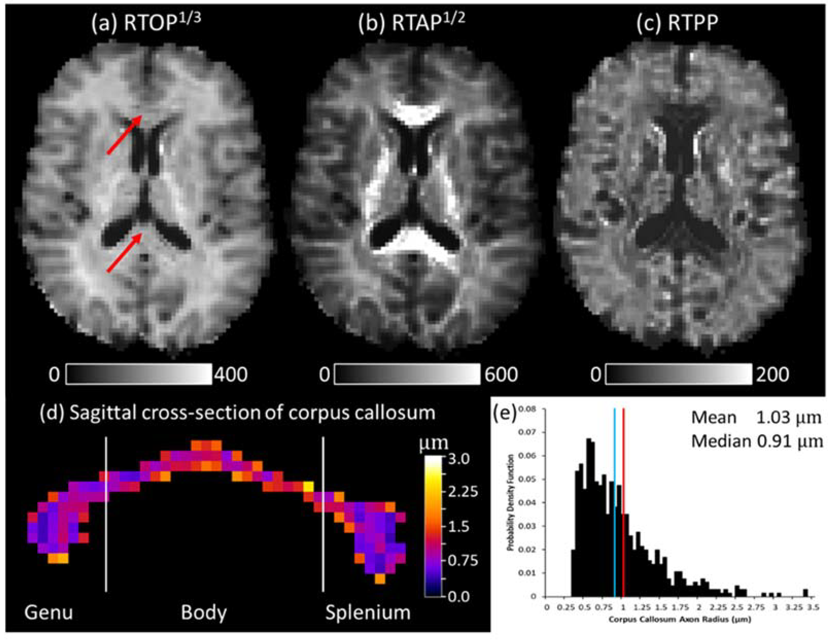
3.1. Quasi-Diffusion Mean Apparent Propagator Imaging of the Corpus Callosum

The corpus callosum is a large commissural white matter bundle that connects cortical regions in the left and right cerebral hemispheres of the brain. The structure of the corpus callosum is such that it does not intersect with other white matter bundles through the interhemispheric fissure (which is in the mid-sagittal plane of the brain). This means that dMRI measurements obtained where the corpus callosum crosses the interhemispheric fissure are only indicative of white matter tissue microstructure in the corpus callosum. In this example, we apply quasi-diffusion MAP imaging to estimate axon radii within a mid-sagittal section of the corpus callosum.

Diffusion MRI data were acquired on a healthy 27-year-old subject using a 3T clinical MR scanner at SGUL. Images were acquired with isotropic voxel size of 2 mm in 10 min 48 s. Data were acquired at $b=\left\{0, 1100,4000\right\}$ s mm⁻² in 32 non-collinear diffusion encoding directions equally spaced on the sphere with $\delta =28.7$ ms and $\mathsf{\Delta }=43.9$ ms, giving an effective diffusion time of $\overline{\mathsf{\Delta }}=34.33$ ms. Full data acquisition details are provided in Appendix A.

Axial, radial and mean $D_{1,2}$ and $\alpha$ values were estimated using quasi-diffusion tensor imaging (QDTI) [1]. QDTI uses a Levenberg–Marquardt algorithm and Padé approximation of the Mittag–Leffler function and its partial derivatives to estimate $D_{1,2}$ and $\alpha$ values in radial lines through q-space [1,65]; $3\times 3$ tensors are fitted to the estimated $D_{1,2}$ and $\alpha$ values to provide matrix representations of $D_{1,2}$ and $\alpha$ as closed quadric surfaces in ${ℝ}^3$ (i.e., ellipsoids or spheres) [1,66]. Eigenvalues ($\lambda \in ℝ$, ${\lambda }_1>{\lambda }_2>{\lambda }_3)$and eigenvectors ($v\in {ℝ}^3)$ are then calculated for the $D_{1,2}$ and $\alpha$ tensors within each voxel. The eigenvector corresponding to ${\lambda }_1$ is considered to be parallel with the gross orientation of tissue microstructure within the voxel, with the remaining eigenvectors providing the orientation of the microstructural cross-section. Axial, radial and mean values for $D_{1,2}$ and $\alpha$ can then be calculated. For example, for the diffusion coefficient we have: axial $D_{1,2}=$ ${\lambda }_1$, radial $D_{1,2}=\left({\lambda }_2+{\lambda }_3\right)/2$ and mean $D_{1,2}=$ $\left({\lambda }_1+{\lambda }_2+{\lambda }_3\right)/3$. $RTOP$, $RTAP$, $RTPP$ and effective mean pore radius were then computed.

Figure 5 shows $RTOP$ (Figure 5a), $RTAP$ (Figure 5b) and $RTPP$ (Figure 5c) maps in an axial slice through the corpus callosum. A sagittal cross-section through the mid-plane of the corpus callosum is shown in Figure 5d. The pseudo colour map indicates estimated axon radii in microns. A histogram of axon radii through a 10 mm thick sagittal section of the corpus callosum is shown in Figure 5e. This indicates axon radii are between 0.25 μm and 3.5 μm (mean 1.03 μm, standard deviation 0.5 μm, median 0.91 μm) with larger radii in the body than the genu and splenium. These measurements are in accordance with histological studies [67].

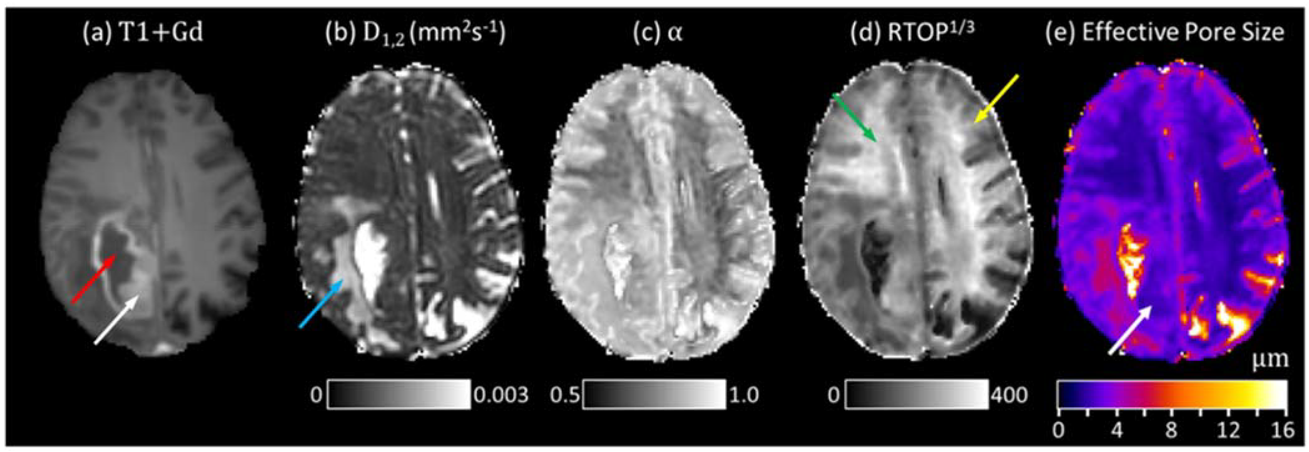
3.2. Quasi-Diffusion Imaging of Brain Tumour

As quasi-diffusion imaging can be acquired in 120 s with high signal to noise ratios [1], it could be feasibly acquired in the clinic. Here we consider an application of quasi-diffusion imaging to a high-grade glial tumour, the glioblastoma multiforme (GBM). Clinical assessment of glial tumour grade and genetic subtype is relevant for predicting patient survival time and treatment strategy which includes surgical resection, chemo- and radiotherapy, and the need for accurate delineation of tumour tissue boundaries [68,69].

Diffusion MRI data were acquired using a 3T clinical MR scanner at SGUL. Images were acquired with a voxel size of $1.5$ mm $\times 1.5$ mm $\times 5$ mm in 120 s. Data were acquired at $b=\left\{0, 1100, 5000\right\}$ s mm⁻² in 6 non-collinear diffusion encoding directions equally spaced on the sphere with $\mathsf{\delta }=23.5$ ms, and $\mathsf{\Delta }=43.7$ ms, giving an effective diffusion time of $\overline{\mathsf{\Delta }}=35.9$ ms. Full patient and data acquisition details are provided in Appendix A. Image analysis was performed using the same techniques as Section 3.1 with the exception that effective mean spherical pore radius was calculated.

In Figure 6, we compare the standard clinical Gadolinium contrast-enhanced T1-weighted (T1wGd) image with parameters derived from quasi-diffusion imaging. In the T1wGd image (Figure 6a), the hyperintense region is typical for GBM and indicates the high-grade tumour core region (where there is angiogenesis and breakdown of the blood-brain barrier) that would be the target for resection and/or highest radiotherapy dose; the central dark region is necrotic tissue. Surrounding this region is the area of tumour infiltration and oedema that is hypointense on the T1wGd image, and is more clearly seen as elevated D_1,2 values (Figure 6b). This region plus a 2 cm margin would be the target for radiotherapy. The quasi-diffusion imaging maps provide different image contrasts with potential to distinguish these regions from a single image modality. Elevated α is evident across the whole lesion (Figure 6c) indicating that the oedema and tumour core are less structured than normal white matter. In addition, α and RTOP^1/3 (Figure 6d) allow distinction between grey and white matter for which contrast is present in the T1wGd image but not the D_1,2 map. Within the RTOP^1/3 hypointense region that delineates tumour oedema/infiltration, there is an area of elevated signal relating to T1wGd enhancement, which is a result of the presence of a greater density of tumour microstructure. Within the T1wGd enhancing region, the effective pore size is approximately 2.5 µm (Figure 6e).

4. Discussion

We have described the mathematical properties of quasi-diffusion, a special case of the CTRW diffusion model and presented the form of its Laplace and Fourier transforms. These functional forms provide insight into the behaviour and interpretation of quasi-diffusion as a model of effective normal diffusion dynamics within a dMRI voxel. The quasi-diffusion equations provide a functional form describing diffusion in MRI. Together, the diffusion coefficient and fractional exponent of the quasi-diffusion characteristic equation define the form of the inverse Laplace transform which provides a spectrum of Fickian diffusivities, and an explicit form for the propagator.

In dMRI, there have been several attempts to describe the functional form of the signal attenuation [8,9,12,13]. Unlike quasi-diffusion, these applied representations and models have not previously provided a simple functional form from which both the inverse Laplace transform and inverse Fourier transform of the signal can be derived. The quasi-diffusion model is compatible with previous frameworks and models that consider the underlying diffusion process in tissue microstructure to be locally Fickian [33,34,35] and lead to a signal that decays with a negative power law [13,19,33,34,35,67]. In the CTRW model, the assumption of a Gaussian scaling relationship between the fractional exponents of time, $\alpha$, and space, $\beta$, leads to a mean-squared displacement that is linearly proportional to time. This leads to the quasi-diffusion model, that is valid in an image voxel beyond the short diffusion time limit, and prior to the long diffusion time limit where tortuosity effects will dominate signal behaviour. For accurate measurement of quasi-diffusion, there is a requirement that diffusing molecules have had sufficient time to explore the microstructural environment.

We consider quasi-diffusion to be the effect of a locally Gaussian diffusion that, within an image voxel, leads to observation of non-Gaussian characteristics due to the ensemble of diffusing molecules being within a heterogeneous environment containing pores with a distribution of structures and radii. The quasi-diffusion model makes no assumptions regarding the shape and distribution of the pores or that diffusing molecules are restricted to locations in the microstructural environment during the diffusion time.

The quasi-diffusion model predicts the existence of dMRI signal at extremely high b-values due to the negative power law behaviour of the stretched Mittag–Leffler function as $b\to {\infty }^{+}$. This prediction is consistent with experimental results that observe signal and power law decay at high diffusion sensitisations of $b=10,000$ s mm⁻² in human white matter in vivo [70], and $b=100,000$ s mm⁻² in rat and human ex vivo corpus callosum [67]. Furthermore, the quasi-diffusion model predicts a stretched exponential form of the signal as $b\to 0^{+}$ consistent with low $b$-values ($b$ < 300 s mm⁻²) containing a significant signal proportion attributable to blood perfusion and a potentially super-diffusive dynamic [71].

The quasi-diffusion signal can be decomposed into a spectrum of Fickian apparent diffusion coefficients via the inverse Laplace transform. Such a transform has been suggested to relate to specific length scales within the diffusion environment [72,73]. Visualisation of the dMRI signal as a diffusion spectrum was first introduced by Yablonskiy et al. [72], where a Gaussian probability density function was assumed. More recently, the assumption of a gamma variate distribution [74] has indicated spectral regions related to pathological changes in disease [74,75,76]. However, each of these studies make assumptions as to the functional form of the probability distribution without supporting evidence. In contrast, the quasi-diffusion model provides a functional form for the spectrum with the $D_{1,2}$ and $\alpha$ parameters together providing an indication of heterogeneity and restriction within the diffusion environment.

The long diffusion times afforded by clinical MR scanners and the complexity of the tissue environment ensure that diffraction patterns from groups of similar pores [11,77] cannot be observed from the dMRI signal [8,78]. Instead, the signal is a relaxation curve with few inherent features. The quasi-diffusion model provides a functional form for the signal which offers an opportunity for developing new quantitative model-based dMRI analysis techniques. We have shown here that the assumption of quasi-diffusion leads to model-based power law and ‘kurtosis’ information, and that the propagator can be applied to obtain MAP images. Possible further applications include use of the diffusion spectrum to provide model-based Multi-dimensional Diffusion MRI [79,80], and use of the propagator to obtain model-based three-dimensional orientation distribution functions of tissue microstructure (similar to those described by [28,81,82,83]) that could be employed within multi-tissue constrained spherical deconvolution techniques for identifying white matter fibre crossing [84].

Advanced diffusion MRI techniques, such as DKI, have been shown to be a sensitive probe of the tissue microstructural environment in healthy and diseased tissue [21,85,86,87,88]. We expect $D_{1,2}$, $\alpha$ and quasi-diffusion MAP images to show a similar sensitivity to disease to previous clinical studies of DKI and MAP imaging. Our examples highlight the potential for quasi-diffusion imaging in clinical research and demonstrate that effective mean pore size measurements may be obtained. Our initial pore size estimations appear to be more accurate in the white matter of the corpus callosum, where the high density of myelinated axons can be considered as isolated pores, than in grey matter and tumour tissue, where more complex distributions of cell structures and shapes are present with permeable membranes, potentially leading to a breakdown of the assumption of isolated pores. Further research is required to determine the efficacy of the quasi-diffusion MAP approach and its clinical potential.

A significant advantage of quasi-diffusion imaging over current dMRI techniques is its ability to provide robust and accurate fits to minimal imaging data [1,55]. This allows acquisition of $D_{1,2}$ and $\alpha$ maps with high signal to noise ratios in a clinically feasible time. New dMRI analysis techniques developed using the quasi-diffusion model will benefit from this advantage, which will potentially enable rapid translation of new techniques from large scale clinical feasibility studies into clinical practice.

There are limitations to the quasi-diffusion imaging technique. For instance, assumption of the short pulse approximation in q-space imaging is generally violated in practice, and the effect of this on measurements is currently unclear. However, the quasi-diffusion model is unique in anomalous dMRI techniques as it does not undermine the Gaussian phase approximation (GPA) [8,11]. Further studies are required to understand the conditions under which quasi-diffusion dynamics emerge within a voxel. In particular, the relationship of the signal to the underlying microstructure, and the effect of the PGSE $\delta$ and Δ on the signal are not well-understood. It is also not yet clear whether the quasi-diffusion model provides imaging measures that are invariant to diffusion time. Nevertheless, the quasi-diffusion model provides a well-defined mathematical basis for further research to elucidate characteristics of the diffusion environment.

5. Conclusions

We have described the mathematics and initial interpretation of the quasi-diffusion model in application to dMRI. This new model of the diffusion dynamics within MRI voxels provides a functional form for the signal from which a diffusion spectrum and propagator can be derived. The quasi-diffusion model is consistent with current understanding of diffusion in tissue microstructure and can be used to provide high quality images of parameters relating to non-Gaussian diffusion in clinically feasible time. The functional form of the quasi-diffusion model represents a novel focus for future mathematical and imaging research. This study shows the potential of quasi-diffusion imaging as a promising new dMRI technique with significant scope for further development.

6. Patents

The quasi-diffusion imaging technique is covered by the patent, “A method and apparatus for quasi-diffusion magnetic resonance imaging”, by inventors Dr. T.R. Barrick, Prof. F.A. Howe, Dr. M.G. Hall, Dr. C. Ingo and Prof. R.L. Magin, WO2021005363A1, filed 8 July 2019, published 14 January 2021.

References

1. Barrick, T.R.; Spilling, C.A.; Ingo, C.; Madigan, J.; Isaacs, J.D.; Rich, P.; Jones, T.L.; Magin, R.L.; Hall, M.G.; Howe, F.A. Quasi-Diffusion Magnetic Resonance Imaging (QDI): A Fast, High b-Value Diffusion Imaging Technique. NeuroImage 2020, 211, 116606. [Google Scholar] [CrossRef]
2. Metzler, R.; Klafter, J. The Random Walk’s Guide to Anomalous Diffusion: A Fractional Dynamics Approach. Phys. Rep. 2000, 339, 1–77. [Google Scholar] [CrossRef]
3. Gorenflo, R.; Mainardi, F. Continuous Time Random Walk, Mittag–Leffler Waiting Time and Fractional Diffusion: Mathematical Aspects. In Anomalous Transport; John Wiley & Sons, Ltd.: Hoboken, NJ, USA, 2008; pp. 93–127. ISBN 978-3-527-62297-9. [Google Scholar]
4. Meerschaert, M.; Scheffler, H.P. Continuous time random walks and space-time fractional differential equations. In Basic Theory; Kochubei, A., Luchko, Y., Eds.; De Gruyter: Berlin, Germany; Boston, MA, USA, 2019; pp. 385–406. ISBN 978-3-11-057162-2. [Google Scholar]
5. Gorenflo, R.; Kilbas, A.A.; Mainardi, F.; Rogosin, S. Applications to Stochastic Models. In Mittag–Leffler Functions, Related Topics and Applications; Gorenflo, R., Kilbas, A.A., Mainardi, F., Rogosin, S., Eds.; Springer Monographs in Mathematics; Springer: Berlin/Heidelberg, Germany, 2020; pp. 339–379. ISBN 978-3-662-61550-8. [Google Scholar]
6. Jones, D.K. Diffusion MRI; Oxford University Press: Oxford, UK, 2010; ISBN 978-0-19-970870-3. [Google Scholar]
7. Johansen-Berg, H.; Behrens, T.E.J. Diffusion MRI: From Quantitative Measurement to In Vivo Neuroanatomy; Academic Press: Cambridge, MA, USA, 2013; ISBN 978-0-12-405509-4. [Google Scholar]
8. Grebenkov, D.S. From the Microstructure to Diffusion NMR, and Back. In Diffusion NMR of Confined Systems; RSC Publishing: Cambridge, UK, 2016; Chapter 3; pp. 52–110. [Google Scholar]
9. Novikov, D.S.; Kiselev, V.G.; Jespersen, S.N. On Modeling. Magn. Reson. Med. 2018, 79, 3172–3193. [Google Scholar] [CrossRef] [PubMed]
10. Afzali, M.; Pieciak, T.; Newman, S.; Garyfallidis, E.; Özarslan, E.; Cheng, H.; Jones, D.K. The Sensitivity of Diffusion MRI to Microstructural Properties and Experimental Factors. J. Neurosci. Methods 2021, 347, 108951. [Google Scholar] [CrossRef]
11. Callaghan, P.T. Principles of Nuclear Magnetic Resonance Microscopy; Clarendon Press: Oxford, UK, 1993; ISBN 978-0-19-853997-1. [Google Scholar]
12. Hall, M.G. The MR Physics of Advanced Diffusion Imaging. In Proceedings of the Computational Diffusion MRI; Fuster, A., Ghosh, A., Kaden, E., Rathi, Y., Reisert, M., Eds.; Springer International Publishing: Cham, Switzerland, 2017; pp. 1–20. [Google Scholar]
13. Magin, R.L.; Abdullah, O.; Baleanu, D.; Zhou, X.J. Anomalous Diffusion Expressed through Fractional Order Differential Operators in the Bloch–Torrey Equation. J. Magn. Reson. 2008, 190, 255–270. [Google Scholar] [CrossRef] [PubMed]
14. Bennett, K.M.; Schmainda, K.M.; Bennett, R.; Rowe, D.B.; Lu, H.; Hyde, J.S. Characterization of Continuously Distributed Cortical Water Diffusion Rates with a Stretched-Exponential Model. Magn. Reson. Med. 2003, 50, 727–734. [Google Scholar] [CrossRef] [PubMed]
15. Hall, M.G.; Barrick, T.R. From Diffusion-Weighted MRI to Anomalous Diffusion Imaging. Magn. Reson. Med. 2008, 59, 447–455. [Google Scholar] [CrossRef]
16. Palombo, M.; Gabrielli, A.; De Santis, S.; Cametti, C.; Ruocco, G.; Capuani, S. Spatio-Temporal Anomalous Diffusion in Heterogeneous Media by Nuclear Magnetic Resonance. J. Chem. Phys. 2011, 135, 034504. [Google Scholar] [CrossRef] [Green Version]
17. Capuani, S.; Palombo, M.; Gabrielli, A.; Orlandi, A.; Maraviglia, B.; Pastore, F.S. Spatio-Temporal Anomalous Diffusion Imaging: Results in Controlled Phantoms and in Excised Human Meningiomas. Magn. Reson. Imaging 2013, 31, 359–365. [Google Scholar] [CrossRef] [Green Version]
18. Bueno-Orovio, A.; Teh, I.; Schneider, J.E.; Burrage, K.; Grau, V. Anomalous Diffusion in Cardiac Tissue as an Index of Myocardial Microstructure. IEEE Trans. Med. Imaging 2016, 35, 2200–2207. [Google Scholar] [CrossRef]
19. Ingo, C.; Magin, R.L.; Colon-Perez, L.; Triplett, W.; Mareci, T.H. On Random Walks and Entropy in Diffusion-Weighted Magnetic Resonance Imaging Studies of Neural Tissue. Magn. Reson. Med. 2014, 71, 617–627. [Google Scholar] [CrossRef] [PubMed] [Green Version]
20. Karaman, M.M.; Sui, Y.; Wang, H.; Magin, R.L.; Li, Y.; Zhou, X.J. Differentiating Low- and High-Grade Pediatric Brain Tumors Using a Continuous-Time Random-Walk Diffusion Model at High b-Values. Magn. Reson. Med. 2016, 76, 1149–1157. [Google Scholar] [CrossRef] [PubMed] [Green Version]
21. Tang, L.; Zhou, X.J. Diffusion MRI of Cancer: From Low to High b-Values. J. Magn. Reson. Imaging JMRI 2019, 49, 23–40. [Google Scholar] [CrossRef] [PubMed] [Green Version]
22. Zhong, Z.; Merkitch, D.; Karaman, M.M.; Zhang, J.; Sui, Y.; Goldman, J.G.; Zhou, X.J. High-Spatial-Resolution Diffusion MRI in Parkinson Disease: Lateral Asymmetry of the Substantia Nigra. Radiology 2019, 291, 149–157. [Google Scholar] [CrossRef]
23. Gatto, R.G.; Ye, A.Q.; Colon-Perez, L.; Mareci, T.H.; Lysakowski, A.; Price, S.D.; Brady, S.T.; Karaman, M.; Morfini, G.; Magin, R.L. Detection of Axonal Degeneration in a Mouse Model of Huntington’s Disease: Comparison between Diffusion Tensor Imaging and Anomalous Diffusion Metrics. Magn. Reson. Mater. Phys. Biol. Med. 2019, 32, 461–471. [Google Scholar] [CrossRef]
24. Jensen, J.H.; Helpern, J.A.; Ramani, A.; Lu, H.; Kaczynski, K. Diffusional Kurtosis Imaging: The Quantification of Non-Gaussian Water Diffusion by Means of Magnetic Resonance Imaging. Magn. Reson. Med. 2005, 53, 1432–1440. [Google Scholar] [CrossRef]
25. Jensen, J.H.; Helpern, J.A. MRI Quantification of Non-Gaussian Water Diffusion by Kurtosis Analysis. NMR Biomed. 2010, 23, 698–710. [Google Scholar] [CrossRef] [PubMed]
26. Özarslan, E.; Koay, C.G.; Basser, P.J. Remarks on Q-Space MR Propagator in Partially Restricted, Axially-Symmetric, and Isotropic Environments. Magn. Reson. Imaging 2009, 27, 834–844. [Google Scholar] [CrossRef]
27. Özarslan, E.; Shemesh, N.; Koay, C.G.; Cohen, Y.; Basser, P.J. NMR Characterization of General Compartment Size Distributions. New J. Phys. 2011, 13, 15010. [Google Scholar] [CrossRef]
28. Özarslan, E.; Koay, C.G.; Shepherd, T.M.; Komlosh, M.E.; İrfanoğlu, M.O.; Pierpaoli, C.; Basser, P.J. Mean Apparent Propagator (MAP) MRI: A Novel Diffusion Imaging Method for Mapping Tissue Microstructure. NeuroImage 2013, 78, 16–32. [Google Scholar] [CrossRef] [PubMed] [Green Version]
29. Mao, J.; Zeng, W.; Zhang, Q.; Yang, Z.; Yan, X.; Zhang, H.; Wang, M.; Yang, G.; Zhou, M.; Shen, J. Differentiation between High-Grade Gliomas and Solitary Brain Metastases: A Comparison of Five Diffusion-Weighted MRI Models. BMC Med. Imaging 2020, 20. [Google Scholar] [CrossRef]
30. Le, H.; Zeng, W.; Zhang, H.; Li, J.; Wu, X.; Xie, M.; Yan, X.; Zhou, M.; Zhang, H.; Wang, M.; et al. Mean Apparent Propagator MRI Is Better Than Conventional Diffusion Tensor Imaging for the Evaluation of Parkinson’s Disease: A Prospective Pilot Study. Front. Aging Neurosci. 2020, 12. [Google Scholar] [CrossRef]
31. Boscolo Galazzo, I.; Brusini, L.; Obertino, S.; Zucchelli, M.; Granziera, C.; Menegaz, G. On the Viability of Diffusion MRI-Based Microstructural Biomarkers in Ischemic Stroke. Front. Neurosci. 2018, 12. [Google Scholar] [CrossRef] [Green Version]
32. Roberts, T.A.; Hyare, H.; Agliardi, G.; Hipwell, B.; d’Esposito, A.; Ianus, A.; Breen-Norris, J.O.; Ramasawmy, R.; Taylor, V.; Atkinson, D.; et al. Noninvasive Diffusion Magnetic Resonance Imaging of Brain Tumour Cell Size for the Early Detection of Therapeutic Response. Sci. Rep. 2020, 10, 9223. [Google Scholar] [CrossRef] [PubMed]
33. Novikov, D.S.; Kiselev, V.G. Effective Medium Theory of a Diffusion-Weighted Signal. NMR Biomed. 2010, 23, 682–697. [Google Scholar] [CrossRef] [PubMed]
34. Novikov, D.S.; Fieremans, E.; Jensen, J.H.; Helpern, J.A. Random Walks with Barriers. Nat. Phys. 2011, 7, 508–514. [Google Scholar] [CrossRef] [PubMed] [Green Version]
35. Novikov, D.S.; Jensen, J.H.; Helpern, J.A.; Fieremans, E. Revealing Mesoscopic Structural Universality with Diffusion. Proc. Natl. Acad. Sci. USA 2014, 111, 5088–5093. [Google Scholar] [CrossRef] [PubMed] [Green Version]
36. Cherstvy, A.G.; Safdari, H.; Metzler, R. Anomalous Diffusion, Nonergodicity, and Ageing for Exponentially and Logarithmically Time-Dependent Diffusivity: Striking Differences for Massive versus Massless Particles. J. Phys. Appl. Phys. 2021, 54, 195401. [Google Scholar] [CrossRef]
37. Assaf, Y.; Blumenfeld-Katzir, T.; Yovel, Y.; Basser, P.J. Axcaliber: A Method for Measuring Axon Diameter Distribution from Diffusion MRI. Magn. Reson. Med. 2008, 59, 1347–1354. [Google Scholar] [CrossRef] [PubMed] [Green Version]
38. Assaf, Y.; Basser, P.J. Composite Hindered and Restricted Model of Diffusion (CHARMED) MR Imaging of the Human Brain. NeuroImage 2005, 27, 48–58. [Google Scholar] [CrossRef] [PubMed]
39. Alexander, D.C.; Hubbard, P.L.; Hall, M.G.; Moore, E.A.; Ptito, M.; Parker, G.J.M.; Dyrby, T.B. Orientationally Invariant Indices of Axon Diameter and Density from Diffusion MRI. NeuroImage 2010, 52, 1374–1389. [Google Scholar] [CrossRef]
40. Zhang, H.; Schneider, T.; Wheeler-Kingshott, C.A.; Alexander, D.C. NODDI: Practical in Vivo Neurite Orientation Dispersion and Density Imaging of the Human Brain. NeuroImage 2012, 61, 1000–1016. [Google Scholar] [CrossRef]
41. Li, J.-R.; Nguyen, H.T.; Van Nguyen, D.; Haddar, H.; Coatléven, J.; Le Bihan, D. Numerical Study of a Macroscopic Finite Pulse Model of the Diffusion MRI Signal. J. Magn. Reson. 2014, 248, 54–65. [Google Scholar] [CrossRef] [Green Version]
42. Nguyen, H.T.; Grebenkov, D.; Van Nguyen, D.; Poupon, C.; Le Bihan, D.; Li, J.-R. Parameter Estimation Using Macroscopic Diffusion MRI Signal Models. Phys. Med. Biol. 2015, 60, 3389–3413. [Google Scholar] [CrossRef]
43. Mainardi, F.; Luchko, Y.; Pagnini, G. The Fundamental Solution of the Space-Time Fractional Diffusion Equation. arXiv 2007, arXiv:cond-mat0702419. [Google Scholar]
44. Mainardi, F.; Pagnini, G. Space-Time Fractional Diffusion: Exact Solutions and Probabilistic Interpretation. In The Waves and Stability in Continuous Media; World Scientific: Porto Ercole, Italy, 2002; pp. 296–301. [Google Scholar]
45. Bazhlekova, E. Subordination Principle for Space-Time Fractional Evolution Equations and Some Applications. Integral Transform. Spec. Funct. 2019, 30, 431–452. [Google Scholar] [CrossRef]
46. Bazhlekova, E.; Bazhlekov, I. Subordination Approach to Space-Time Fractional Diffusion. Mathematics 2019, 7, 415. [Google Scholar] [CrossRef] [Green Version]
47. Luchko, Y. Subordination Principles for the Multi-Dimensional Space-Time-Fractional Diffusion-Wave Equation. arXiv 2018, arXiv:180204752. [Google Scholar] [CrossRef] [Green Version]
48. Boyadjiev, L.; Luchko, Y. Multi-Dimensional α-Fractional Diffusion–Wave Equation and Some Properties of Its Fundamental Solution. Comput. Math. Appl. 2017, 73, 2561–2572. [Google Scholar] [CrossRef]
49. Luchko, Y. Entropy Production Rate of a One-Dimensional Alpha-Fractional Diffusion Process. Axioms 2016, 5, 6. [Google Scholar] [CrossRef] [Green Version]
50. Luchko, Y. Entropy Production Rates of the Multi-Dimensional Fractional Diffusion Processes. Entropy 2019, 21, 973. [Google Scholar] [CrossRef] [Green Version]
51. Berberan-Santos, M.N. Properties of the Mittag–Leffler Relaxation Function. J. Math. Chem. 2005, 38, 629–635. [Google Scholar] [CrossRef]
52. Mainardi, F. On Some Properties of the Mittag-Leffler Function E α ( t α ) , Completely Monotone for t > 0 with 0 < α < 1 . Discret. Contin. Dyn. Syst. B 2014, 19, 2267–2278. [Google Scholar] [CrossRef]
53. Mainardi, F. Fractional Calculus and Waves in Linear Viscoelasticity: An Introduction to Mathematical Models; World Scientific: Porto Ercole, Italy, 2010; ISBN 978-1-908978-57-8. [Google Scholar]
54. Ingo, C.; Magin, R.L.; Parrish, T.B. New Insights into the Fractional Order Diffusion Equation Using Entropy and Kurtosis. Entropy 2014, 16, 5838–5852. [Google Scholar] [CrossRef] [PubMed]
55. Spilling, C.A.; Howe, F.A.; Barrick, T.R. Quasi-Diffusion Magnetic Resonance Imaging (QDI): Optimisation of Acquisition Protocol. In Proceedings of the International Society for Magnetic Resonance in Medicine Virtual Conference & Exhibition, Paris, France, 8–13 October 2020; p. 4391. [Google Scholar]
56. Haubold, H.J.; Mathai, A.M.; Saxena, R.K. Mittag-Leffler Functions and Their Applications. J. Appl. Math. 2011, 2011, 1–51. [Google Scholar] [CrossRef] [Green Version]
57. Mainardi, F. Why the Mittag-Leffler Function Can Be Considered the Queen Function of the Fractional Calculus? Entropy 2020, 22, 1359. [Google Scholar] [CrossRef]
58. Gorenflo, R.; Kilbas, A.A.; Mainardi, F.; Rogosin, S. The Classical Mittag-Leffler Function. In Mittag-Leffler Functions, Related Topics and Applications; Gorenflo, R., Kilbas, A.A., Mainardi, F., Rogosin, S., Eds.; Springer Monographs in Mathematics; Springer: Berlin/Heidelberg, Germany, 2020; pp. 19–62. ISBN 978-3-662-61550-8. [Google Scholar]
59. Mainardi, F. Fractional Relaxation-Oscillation and Fractional Diffusion-Wave Phenomena. Chaos Solitons Fractals 1996, 7, 1461–1477. [Google Scholar] [CrossRef]
60. Gorenflo, R.; Kilbas, A.A.; Mainardi, F.; Rogosin, S. Applications to Deterministic Models. In Mittag-Leffler Functions, Related Topics and Applications; Gorenflo, R., Kilbas, A.A., Mainardi, F., Rogosin, S., Eds.; Springer Monographs in Mathematics; Springer: Berlin/Heidelberg, Germany, 2020; pp. 281–337. ISBN 978-3-662-61550-8. [Google Scholar]
61. Gorenflo, R.; Kilbas, A.A.; Mainardi, F.; Rogosin, S. Mittag-Leffler Functions, Related Topics and Applications; Springer: Berlin/Heidelberg, Germany, 2020; ISBN 978-3-662-61549-2. [Google Scholar]
62. Samko, S.G.; Kilbas, A.A.; Marichev, O.I. Fractional Integrals and Derivatives: Theory and Applications; Gordon and Breach Science Publishers: Montreaux, Switzerland; Philadelphia, PA, USA, 1993; ISBN 978-2-88124-864-1. [Google Scholar]
63. Mainardi, F.; Pagnini, G.; Saxena, R.K. Fox H Functions in Fractional Diffusion. J. Comput. Appl. Math. 2005, 178, 321–331. [Google Scholar] [CrossRef] [Green Version]
64. Panagiotaki, E.; Walker-Samuel, S.; Siow, B.; Johnson, S.P.; Rajkumar, V.; Pedley, R.B.; Lythgoe, M.F.; Alexander, D.C. Noninvasive Quantification of Solid Tumor Microstructure Using VERDICT MRI. Cancer Res. 2014, 74, 1902–1912. [Google Scholar] [CrossRef] [Green Version]
65. Ingo, C.; Barrick, T.R.; Webb, A.G.; Ronen, I. Accurate Padé Global Approximations for the Mittag-Leffler Function, Its Inverse, and Its Partial Derivatives to Efficiently Compute Convergent Power Series. Int. J. Appl. Comput. Math. 2017, 3, 347–362. [Google Scholar] [CrossRef]
66. Hall, M.G.; Barrick, T.R. Two-Step Anomalous Diffusion Tensor Imaging. NMR Biomed. 2012, 25, 286–294. [Google Scholar] [CrossRef]
67. Veraart, J.; Nunes, D.; Rudrapatna, U.; Fieremans, E.; Jones, D.K.; Novikov, D.S.; Shemesh, N. Nonivasive Quantification of Axon Radii Using Diffusion MRI. eLife 2020, 9. [Google Scholar] [CrossRef] [PubMed]
68. Bai, J.; Varghese, J.; Jain, R. Adult Glioma WHO Classification Update, Genomics, and Imaging: What the Radiologists Need to Know. Top. Magn. Reson. Imaging 2020, 29, 71–82. [Google Scholar] [CrossRef]
69. Hu, L.S.; Hawkins-Daarud, A.; Wang, L.; Li, J.; Swanson, K.R. Imaging of Intratumoral Heterogeneity in High-Grade Glioma. Cancer Lett. 2020, 477, 97–106. [Google Scholar] [CrossRef]
70. Veraart, J.; Fieremans, E.; Novikov, D.S. On the Scaling Behavior of Water Diffusion in Human Brain White Matter. NeuroImage 2019, 185, 379–387. [Google Scholar] [CrossRef] [PubMed]
71. Reiter, D.A.; Adelnia, F.; Cameron, D.; Spencer, R.G.; Ferrucci, L. Parsimonious Modeling of Skeletal Muscle Perfusion: Connecting the Stretched Exponential and Fractional Fickian Diffusion. Magn. Reson. Med. 2021, 86, 1045–1057. [Google Scholar] [CrossRef]
72. Yablonskiy, D.A.; Bretthorst, G.L.; Ackerman, J.J.H. Statistical Model for Diffusion Attenuated MR Signal. Magn. Reson. Med. 2003, 50, 664–669. [Google Scholar] [CrossRef] [Green Version]
73. Magin, R.L.; Rawash, Y.Z.; Berberan-Santos, M.N. Analyzing Anomalous Diffusion in NMR Using a Distribution of Rate Constants. In Fractional Dynamics and Control; Springer: Berlin, Germany, 2012; pp. 263–274. [Google Scholar]
74. Oshio, K.; Shinmoto, H.; Mulkern, R.V. Interpretation of Diffusion MR Imaging Data Using a Gamma Distribution Model. Magn. Reson. Med. Sci. MRMS Off. J. Jpn. Soc. Magn. Reson. Med. 2014, 13, 191–195. [Google Scholar] [CrossRef] [PubMed] [Green Version]
75. Borlinhas, F.; Loução, R.; Conceição, R.C.; Ferreira, H.A. Gamma Distribution Model in the Evaluation of Breast Cancer Through Diffusion-Weighted MRI: A Preliminary Study. J. Magn. Reson. Imaging JMRI 2019, 50, 230–238. [Google Scholar] [CrossRef]
76. Togao, O.; Chikui, T.; Tokumori, K.; Kami, Y.; Kikuchi, K.; Momosaka, D.; Kikuchi, Y.; Kuga, D.; Hata, N.; Mizoguchi, M.; et al. Gamma Distribution Model of Diffusion MRI for the Differentiation of Primary Central Nerve System Lymphomas and Glioblastomas. PLoS ONE 2020, 15, e0243839. [Google Scholar] [CrossRef]
77. Özarslan, E.; Basser, P.J. MR Diffusion—“Diffraction” Phenomenon in Multi-Pulse-Field-Gradient Experiments. J. Magn. Reson. 2007, 188, 285–294. [Google Scholar] [CrossRef] [PubMed] [Green Version]
78. Avram, L.; Özarslan, E.; Assaf, Y.; Bar-Shir, A.; Cohen, Y.; Basser, P.J. Three-Dimensional Water Diffusion in Impermeable Cylindrical Tubes: Theory versus Experiments. NMR Biomed. 2008, 21, 888–898. [Google Scholar] [CrossRef] [PubMed]
79. Westin, C.-F.; Knutsson, H.; Pasternak, O.; Szczepankiewicz, F.; Özarslan, E.; van Westen, D.; Mattisson, C.; Bogren, M.; O’Donnell, L.J.; Kubicki, M.; et al. Q-Space Trajectory Imaging for Multidimensional Diffusion MRI of the Human Brain. NeuroImage 2016, 135, 345–362. [Google Scholar] [CrossRef] [PubMed] [Green Version]
80. Topgaard, D. Multidimensional Diffusion MRI. J. Magn. Reson. 2017, 275, 98–113. [Google Scholar] [CrossRef] [PubMed]
81. Tuch, D.S. Q-Ball Imaging. Magn. Reson. Med. 2004, 52, 1358–1372. [Google Scholar] [CrossRef]
82. Wedeen, V.J.; Hagmann, P.; Tseng, W.-Y.I.; Reese, T.G.; Weisskoff, R.M. Mapping Complex Tissue Architecture with Diffusion Spectrum Magnetic Resonance Imaging. Magn. Reson. Med. 2005, 54, 1377–1386. [Google Scholar] [CrossRef]
83. Wedeen, V.J.; Wang, R.P.; Schmahmann, J.D.; Benner, T.; Tseng, W.Y.I.; Dai, G.; Pandya, D.N.; Hagmann, P.; D’Arceuil, H.; de Crespigny, A.J. Diffusion Spectrum Magnetic Resonance Imaging (DSI) Tractography of Crossing Fibers. NeuroImage 2008, 41, 1267–1277. [Google Scholar] [CrossRef]
84. Jeurissen, B.; Tournier, J.-D.; Dhollander, T.; Connelly, A.; Sijbers, J. Multi-Tissue Constrained Spherical Deconvolution for Improved Analysis of Multi-Shell Diffusion MRI Data. NeuroImage 2014, 103, 411–426. [Google Scholar] [CrossRef]
85. Kamagata, K.; Andica, C.; Hatano, T.; Ogawa, T.; Takeshige-Amano, H.; Ogaki, K.; Akashi, T.; Hagiwara, A.; Fujita, S.; Aoki, S. Advanced Diffusion Magnetic Resonance Imaging in Patients with Alzheimer’s and Parkinson’s Diseases. Neural Regen. Res. 2020, 15, 1590–1600. [Google Scholar] [CrossRef]
86. Nagaraja, N. Diffusion Weighted Imaging in Acute Ischemic Stroke: A Review of Its Interpretation Pitfalls and Advanced Diffusion Imaging Application. J. Neurol. Sci. 2021, 425, 117435. [Google Scholar] [CrossRef]
87. Raja, R.; Rosenberg, G.; Caprihan, A. Review of Diffusion MRI Studies in Chronic White Matter Diseases. Neurosci. Lett. 2019, 694, 198–207. [Google Scholar] [CrossRef] [PubMed]
88. Delouche, A.; Attyé, A.; Heck, O.; Grand, S.; Kastler, A.; Lamalle, L.; Renard, F.; Krainik, A. Diffusion MRI: Pitfalls, Literature Review and Future Directions of Research in Mild Traumatic Brain Injury. Eur. J. Radiol. 2016, 85, 25–30. [Google Scholar] [CrossRef] [PubMed]
Figure 1. The family of quasi-diffusion imaging signal attenuation curves for an arbitrary diffusion coefficient of D 1 , 2 = 1.5 × 10 3   mm2 s−1 and a range of fractional exponents, 0.1 α 0.99 . Normalised signal is shown parameterised by (a) diffusion-sensitisation, b , and (b) q . Graph (c) shows the power law behaviour of the signal decay parameterised by b on a logarithmic scale.
Mathematics 09 01763 g001
Figure 2. Quasi-diffusion model fits to experimental diffusion magnetic resonance imaging data acquired in the brain of a young, healthy subject (age 28 years). The top row shows the results of fitting the quasi-diffusion model to an acquisition of 29   b -values over the range 0 < b 5000 s mm−2, with the bottom row showing the results of fitting the quasi-diffusion model to 3   b -values, b = { 0 , 1080 , 5000 } s mm−2. All imaging data were acquired in 6 diffusion encoding directions at an effective diffusion time of Δ ¯ = 35.9 ms. Normalised signal attenuation is shown for a grey matter voxel indicated by the blue arrow (graphs (a,e)), and a white matter voxel indicated by the red arrow (graphs (b,f)). Axial slices are shown for maps of mean D 1 , 2 (images (c,g)) and mean α (images (d,h)).
Mathematics 09 01763 g002
Figure 3. Decomposition of the signal into a spectrum of Fickian apparent diffusion coefficients via the inverse Laplace transform. Graph (a) shows the probability density functions for a unit diffusion coefficient, D 1 , 2 = 1   mm2 s−1 for different fractional exponents, 0.1 α 0.99 . Spectra are shown for axial, radial and mean D 1 , 2 and α values in (b) cerebrospinal fluid, (c) grey matter and (d) white matter. D 1 , 2 and α values used to calculate the spectra are from Barrick et al. [1].
Mathematics 09 01763 g003
Figure 4. The one-dimensional quasi-diffusion propagator for an arbitrary diffusion coefficient, D 1 , 2 = 1.5 × 10 3 mm2 s−1 for 0.5 α 0.99 . The one-dimensional probability density function is shown (a) in space at an effective diffusion time of Δ ¯ = 35.9 ms, and (b) in time at x = 5 μm.
Mathematics 09 01763 g004
Figure 5. Quasi-diffusion mean apparent propagator imaging results for a young, healthy subject (age 27 years). The top row shows axial slices through (a) R T O P 3 , (b) R T A P , and (c) R T P P maps. The bottom row shows (d) effective pore radius estimates in a cross-section through the mid-sagittal plane of the corpus callosum, and (e) a probability density function of micron radii for the analysed 10 mm thick section of the corpus callosum (graph (e)). The location of the corpus callosum is identified by red arrows. The red and blue lines in graph (e) indicate the mean and median, respectively.
Mathematics 09 01763 g005
Figure 6. Quasi-diffusion imaging results for axial slices through a high-grade glial tumour (WHO Grade IV glioblastoma). Diffusion magnetic resonance imaging data were acquired at b = { 0 ,   1100 , 5000 } s mm−2 in 6 diffusion encoding directions at an effective diffusion time of Δ ¯ = 35.9 ms. Imaging data were acquired in a clinically feasible time of 120 s. Image (a) shows a T1-weighted image acquired after injection of gadolinium contrast agent, with maps of (b) mean D 1 , 2 , (c) mean α , (d) R T O P 3 and (e) effective mean pore size, R , (which in the absence of oedema or necrosis will relate to cell size). Arrows indicate the following regions: white—tumour core, red—necrosis, blue—oedema, yellow—grey matter, green—white matter.
Mathematics 09 01763 g006
Publisher’s Note: MDPI stays neutral with regard to jurisdictional claims in published maps and institutional affiliations.