Article

A Surrogate Model-Based Hybrid Approach for Stochastic Robust Double Row Layout Problem

1
School of Computer Science, Beijing University of Posts and Telecommunications, Beijing 100876, China
2
Key Laboratory of Trustworthy Distributed Computing and Service, Ministry of Education, Beijing 100876, China
3
School of Science, Beijing University of Posts and Telecommunications, Beijing 100876, China
*
Author to whom correspondence should be addressed.
Mathematics 2021, 9(15), 1711; https://doi.org/10.3390/math9151711
Submission received: 30 June 2021 / Revised: 14 July 2021 / Accepted: 16 July 2021 / Published: 21 July 2021

Abstract

:
The double row layout problem is to arrange a number of machines on both sides of a straight aisle so as to minimize the total material handling cost. Aiming at the random distribution of product demands, we study a stochastic robust double row layout problem (SR-DRLP). A mixed integer programming (MIP) model is established for SR-DRLP. A surrogate model is used to linearize the nonlinear term in the MIP to achieve a mixed integer linear programming model, which can be readily solved by an exact method to yield high-quality solutions (layouts) for small-scale SR-DRLPs. Furthermore, we propose a hybrid approach combining a local search and an exact approach (LS-EA) to solve large-scale SR-DRLPs. Firstly, a local search is designed to optimize the machine sequences on two rows and the clearance from the most left machine on row 1 to the left boundary. Then, the exact location of each machine is further optimized by an exact approach. The LS-EA is applied to six problem instances ranging from 8 to 50 machines. Experimental results show that the surrogate model is effective and LS-EA outperforms the comparison approaches.

1. Introduction

Research on the facility layout problem (FLP) usually involves the arrangement of machines in a plant, which is of great significance for improving production efficiency and reducing cost [1]. The three most commonly used material handling devices in FLP [2,3] are gantry robot, automated guided vehicle (AGV) and handling robot. Due to the outstanding performance of the AGV in terms of utilization and flexibility, it is commonly selected to link pairs of machines in FLP. To simplify the material handling, AGVs are restricted to move along a bi-directional straight line and machines are usually placed on one or both sides of the straight aisle. The double row layout problem (DRLP) is to locate machines on both sides of a straight aisle to minimize the material handling cost, and has a wide range of applications in semiconductor manufacturing [4] and LCD fabrication lines [5].
In DRLP, there are material interactions amongst machines on the same side and/or on different sides. Zuo et al. [4] showed that separating adjacent machines with a suitable clearance larger than the minimum could achieve a layout with lower material flow cost. Therefore, a solution to DRLP involves the machine sequence on each row, and the exact location of each machine on its assigned row (i.e., the extra clearance of each machine). That makes the DRLP more difficult to solve.
In FLPs with the aim of minimizing total material handling cost, the material flows amongst machines directly affect the performance of the layout. In practice, product demands dynamically change so as to meet the personalized needs of users, resulting in the material flows amongst machines changing over time. To our knowledge, there are only two studies on DRLP in dynamic production environments. Wang et al. [6] studied a dynamic double row layout problem, where multiple processing periods are considered and material flows amongst machines are fixed during a specific period but change over different periods. They sought to design an effective layout for each processing period to minimize the sum of the material handling cost and the rearrangement cost of machines relocated in consecutive periods. The dynamic layout problem usually involves considerable rearrangement and time costs due to production interruption, while a robust layout is able to deal with different processing periods well. Tang et al. [7] studied a robust double row layout problem that minimizes material handling cost and layout area simultaneously.
All existing studies on DRLP assume that material flows amongst machines are predefined and known. However, it is difficult to accurately forecast specific product demands, due to the uncertainty of market demands. According to the historical trend of product demands, employing a random variable to describe them is more realistic. The normal distribution is one of the most commonly used statistical distributions for this [8,9].
In this paper, we study a stochastic double row layout problem (SR-DRLP), which involves multiple processing periods, and product demands are independent normally distributed random variables. We focus on finding a robust layout which can handle different processing periods. Firstly, a mixed integer programming (MIP) model is established for SR-DRLP. To linearize the nonlinear term in the MIP, we build a linear model to fit the nonlinear term. A collection of training data is obtained by randomly generated layouts to the SR-DRLP, in order to train the linear model. Then, the linear model (termed surrogate model) is employed to replace the nonlinear term in order to make the MIP a mixed integer linear programming model, which can be utilized to find high-quality solutions to small-scale SR-DRLPs by an exact method. Then, a hybrid approach combining a local search and an exact approach (LS-EA) is proposed to solve large-scale SR-DRLPs. Firstly, the local search is designed to determine the sequence of all machines, the number of machines on row 1 (abbreviated as breakpoint) and the clearance from the left-most machine on row 1 to the left boundary (abbreviated as offset). Subsequently, utilizing the linearized MIP, the exact location of each machine is optimized by the exact approach.

2. Related Literature

FLP refers to determining the locations of machines in a plant, and plays an important role in manufacturing systems in terms of improving production efficiency and reducing operating costs [10]. Several recent reviews on FLP have been published [11,12]. There are two types of layout design closely related to DRLP, the parallel row ordering problem (PROP) and the space-free double-row facility layout problem (SF-DRLP).
Double row layout problem. In DRLP, a machine can be located anywhere on either of the two rows. Thus, there are three sub-problems in DRLP, i.e., the allocation of machines on the two rows, the sequence of machines on each row and the exact locations of these machines. Chung and Tanchoco [5] added more variables and constraints to the existing formulations of the single row layout problem and developed a mixed integer programming model for DRLP. In addition, a high-quality initial solution and corresponding upper bound of DRLP was provided by five proposed heuristic algorithms. However, the mixed integer programming model ignores the clearance constraint between adjacent machines, which may result in an illegal solution. A corrected formulation was proposed by Zhang and Murray [13]. Amaral [14] proposed a mixed integer programming formulation based on the α-incidence vectors for DRLP, where the implicit clearances are considered. This can provide a solution for the DRLP with up to 12 machines. Later, Secchin and Amaral [15] modified the mixed integer programming model in [14] and proposed a tighter model. This modified model can be utilized to solve the DRLP with up to 15 machines. Chae and Reganb [16] proposed a model for DRLP, which is modified from the model in [15]. The model greatly reduces the calculation time and solves DRLP with 16 machines. Amaral [17] established a mixed integer programming model for DRLP, which includes valid inequalities and a symmetry-breaking constraint. The model is more intuitive for handling qualitative inputs. Dahlbeck [18] presented combinatorial lower bounds for DRLP, and combined these lower bounds with a new distance-based mixed integer linear programming model to improve the lower bounds. Amaral [19] established a mixed integer programming model for DRLP based on a linear extension of a partial order on the set of machines. Compared with previously published models in the literature, this mode has the least number of 0–1 variables. All the above studies seek to obtain the optimal solution to DRLP by establishing a mathematical programming model.
To obtain a satisfactory solution for large-scale DRLP, some heuristic algorithms have been proposed. Zuo et al. [4] studied an extended DRLP where nonzero aisle widths are allowed and two optimization objectives are considered (cost and layout area). Moreover, they proposed an approach combining multi-objective tabu search with linear programming for the extended DRLP. Gülşen et al. [20] studied a variant of DRLP, where multiple replicates of the same machine allow the product flows to split into multiple parallel flow lines. For this problem, they established a nonlinear mixed integer programming formulation and developed a hierarchical heuristic to determine machine placements and corresponding material flows. Guan [21] proposed a decomposition-based algorithm for DRLP. First, a local search was applied to optimize machine sequences on two rows and the difference between two starting abscissas. Then, the clearances between adjacent machines were optimized by a particle swarm optimization. Murray [22] studied the DRLP with asymmetric material flows and established a mixed integer linear programming model. The problem was solved by a combination of a constructive heuristic and a local search. Amaral [23] presented four variants of a two-phase algorithm for a DRLP, where the width of aisle between two rows is negligible and required minimal clearance between any two machines is a constant. First, an improvement heuristic was devised to optimize the machine sequence and the leftmost point of the arrangement at row 1. Then, the machine location was further optimized by a linear programming.
For the dynamic processing environment in practice, in our previous work we studied a dynamic DRLP, where a layout was designed for each processing period to minimize total material flow cost and rearrangement cost [6], and proposed a robust layout method for a robust DRLP [7]. In all the above studies on DRLP, the material flows amongst machines are predefined and known.
Parallel row ordering problem. The PROP is an extended version of the single-row layout problem (SRLP) and considers the arrangements of facilities along two parallel rows. In PROP, facilities with certain characteristics in common are placed on one row, and the remaining facilities are arranged on a parallel row. Moreover, the arrangements of facilities on both rows have a common left origin and there is no clearance allowed between adjacent facilities on the same row. The objective of PROP is to find a facility sequence on each row to minimize the total material handling cost. Amaral [24] presented a mixed integer programming model for PROP, which extends a mixed integer programming formulation of the SRLP. Since PROP has fewer constraints and binary variables than SRLP, the PROP can be solved faster. Yang et al. [25] proposed a mixed integer programming model for PROP, which modifies some constraints of the model in [24]. Gong et al. [26] studied a dynamic PROP considering variable inter-facility material flow. The objective is to minimize the sum of the material handling cost and the rearrangement cost. They developed a hybrid algorithm of harmony search and tabu search to solve larger-scale PROPs.
Space-free double-row facility layout problem. The PROP is further extended to a SF-DRLP (also called the corridor allocation problem, CAP), in which the facilities can be placed on any of two rows. The SF-DRLP does not restrict the row to which facilities are allocated, so that SF-DRLP is more complicated than PROP. Amaral [27] first investigated SF-DRLP and proposed a mixed integer programming formulation that can be solved in reasonable time for moderate-scale problem instances. Moreover, three heuristic procedures were presented to handle larger-scale problem instances. Ahonen [28] presented a tabu search and a simulated annealing algorithm for SF-DRLP to minimize the sum of weighted distances. Kalita et al. [29] applied a permutation-based genetic algorithm to handle SF-DRLP, with the objective of minimizing the total material handling cost and the length of the corridor. Kalita et al. [30] further studied a bi-objective SF-DRLP and proposed a permutation-based genetic algorithm incorporating a promising local search technique to solve SF-DRLP. Zhang et al. [31] established a mixed integer programming model for SF-DRLP, which considers the effect of the corridor width. Moreover, they proposed an improved scatter search algorithm for SR-DRLP, which includes several improvement mechanisms, such as the adoption of a simulated annealing operation, a dynamic reference set update method, and an improved subset generation. Fischer [32] presented a mixed integer linear programming formulation for SF-DRFLP to solve instances with 16 machines.

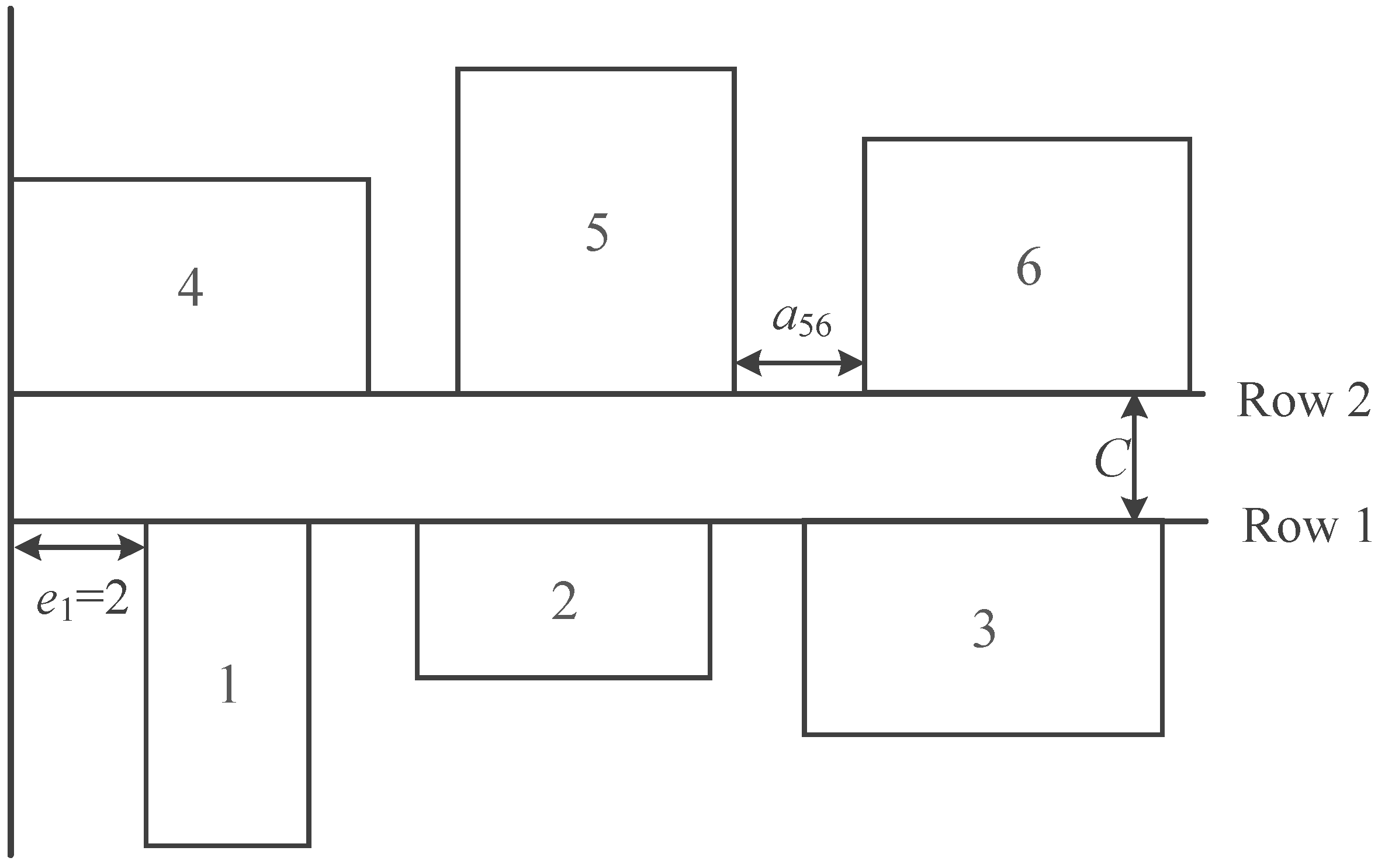
3. Problem Description

SR-DRLP involves producing a series of different types of products in multiple processing periods and determining the locations of machines participating in the production task on two rows R = {1, 2}. Let L = { 1 , 2 , , l }, T = { 1 , 2 , , t } and M = { 1 , 2 , , m }, respectively, represent the sets of product types, processing periods and machines, where l, t, and m denote the number of the product types, processing periods and machines, respectively. The demands of product p L in processing period c T are denoted by Dcp. Assume that product demands Dcp are independent and normally distributed with known expected value E(Dcp) and variance Var(Dcp). Each machine i M is a rectangle with fixed width wi and depth di. The processing technology of the product p is represented by Bijp, such that Bijp = 1 if product p L is processed on machine i M and then immediately processed on machine j M \ { i } , otherwise Bijp = 0. Each pair of machines on the same row i M and j M \ { i } must satisfy a minimum clearance constraint aij. In addition to the minimum clearance aij, there may be an extra clearance ej either between machines i M and j M \ { i } or between machine i M and the left side of the layout boundary. The load/unload station of the machine is located at the center of its predefined side. The width of aisle between two rows is represented C. The distance of each pair of machines is measured by their rectilinear distance between their load/unload stations. The optimization objective is to determine the location of each machine to minimize the total material flow cost in all the t periods.
Figure 1 shows an example of layout for SR-DRLP, which includes six machines and two rows. In this case, machines 1, 2 and 3 (4, 5 and 6) are location on row 1 (row 2). The width and depth of machine 6 are w6 and d6, respectively. Machines 1 and 2 are on the same row and they are separated by a minimum clearance of them a1,2 and an extra clearance e2. The distance between machine 6 and machine 2 is L2,6 = x6x2 + C, where x6 and x2 are the abscissas of machines 6 and 2, respectively.
The decision variables of SR-DRLP are listed in Table 1.
Derakhshan et al. [8] established a mixed integer programming model for an unequal-area stochastic facility layout problem. Based on the work in [8], we formulate a mixed integer programming model for SR-DRLP.
Minimize M H C = c = 1 t i = 1 m j = 1 m p = 1 l β i j p E ( D c p ) ( v i j + v i j + + C ( 1 s i j ) ) + Z 1 α c = 1 t i = 1 m j = 1 m p = 1 l β i j p 2 V a r ( D c p ) ( v i j + v i j + + C ( 1 s i j ) ) 2
Subject   to : x i x j = v i j v i j + i M , j M \ { i }
q i 1 + q i 2 = 1 i M
w i q i r + w j q j r 2 + a i j z j i r x i x j + U ( 1 z j i r ) i M , j M \ { i }
z i j r + z j i r q i r i M , j M \ { i }
z i j r + z j i r + 1 q i r + q j r i M , j M \ { i }
r R z i j r + r R z j i r = s i j i M , j M \ { i }
q 11 = 1
x 1 x 2
x i 0 , v i j , v i j + 0 i M , j M \ { i }
q i r , s i j , z i j r { 0 , 1 } i M , j M \ { i }
The material handling cost of SR-DRLP is given by Equation (1), where the Z1-α is the standard normal Z value at confidence level 1-α. Constraint (2) is employed to determine the distance between a pair of machines. Constraint (3) ensures that one, and only one, row is selected for each machine to be located. The minimum clearance constraint between each pair of machines on the same row is defined by Equation (4). U is a sufficiently large constant. Constraints (5) and (6) relate binary decision variables zijr and qir. Constraint (7) is used to judge whether any two machines are on the same row.
The layout (solution) to SR-DRLP is symmetry, i.e., rotating a layout by 180° or swapping the machine sequences on two rows can result in a layout with the same material handling cost as the original layout. There are three equivalent layouts for each layout, as shown in Figure 2. If this symmetry can be broken, the size of the decision space can be greatly reduced. Constraints (8) and (9) are utilized to break the symmetry, i.e., we add the following constraints: machine 1 is placed on row 1 and the abscissa of machine 1 is smaller than the abscissa of machine 2. Equations (10) and (11) define the ranges of decision variables.

4. Proposed Approach

For the SR-DRLP, a feasible layout contains the machine sequence on each row and the exact location of each machine on its row. SR-DRLP is NP-hard due to involving the machine sorting task. Local search is an effective heuristic approach for combinatorial optimization problems and there are many studies [33,34,35] that apply this to solve FLPs. In this paper, we propose a hybrid approach combining a local search and an exact approach (LS-EA) to solve SR-DRLP.
LS-EA includes two stages: (1) a local search is proposed to determine the sequence of all machines, breakpoint and offset for the SR-DRLP; (2) EA is employed to optimize the exact locations of machines of the solution found by the LS, and the optimal extra clearance of each machine is identified.

4.1. Local Search Algorithm

Amaral [23] presented four heuristics for DRLP without minimum clearance between any two adjacent machines. The fourth heuristic optimized the machine sequence, the number of machines on row 1 and the leftmost point of the arrangement at row 1. In this heuristic, each feasible solution corresponds to a layout, where there is no clearance between any adjacent machines and the leftmost point of the arrangement at row 2 is fixed at zero. Based on this heuristic, we devise a local search for SR-DRLP with the following improvements:
(1) Let the range of the offset be an equally spaced vector with values from 0 to maxO and the range of the breakpoint be in [ m / 2 ,   m a x B ] , where maxO and maxB are predefined parameters corresponding to the maximum value of offset and breakpoint, respectively. Then, all possible combinations of offset and breakpoint are traversed. For each combination, a 2-opt local search with the first improvement search strategy is employed to improve the machine sequence. The final solution is the best solution amongst all solutions found by 2-opt local search for all possible combinations of offset and breakpoint. Traversing all combinations aims to avoid falling into the local optima during the search of offset and breakpoint.
(2) In the 2-opt local search, we add an additional step to improve the global search capability. That is, in each iteration, we first generate all neighbor solutions by swapping the positions of machines, and then randomly shuffle the order of neighbor solutions.

4.1.1. Encoding and Decoding

In the LS, a feasible solution of SR-DRLP is represented by a coding (π, b, o), where π denotes the sequence of all machines; b is the breakpoint that identifies the number of machines on row 1 such that (m-b) machines are on row 2; and o is the offset that indicates the clearance from the most left machine on row 1 to the left boundary (i.e., the extra clearance of the leftmost machine on row 1). For a feasible solution in the LS, the extra clearances of all machines are zero except the leftmost machine on row 1.
The decoding procedure is to convert a coding (π, b, o) into a layout. To clearly describe the decoding process, we take a coding (π = {1, 2, 3, 4, 5, 6}, b = 3, o = 2) as an example to illustrate the decoding process, as shown in Figure 3. As b is 3, the first three machines {1, 2, 3} in π are placed on row 1 from left to right one by one and there is no extra clearance for each machine, i.e., adjacent machines on the same row are separated by their minimum clearance. The next three machines {4, 5, 6} are places on row 2 in the same manner. The extra clearance of the left most machine on row 1 is the value of o, i.e., e1 = 2.

4.1.2. Local Search Algorithm

The pseudo-code of the LS is presented in Algorithm 1. The LS starts with an initial solution y = (π, m/2, 0), where π is a random permutation of all machines. The material handling cost of y, f(y), is computed by Equation (1). For each candidate combination of b and o, the breakpoint and offset in y are first updated to b and o, respectively. Then y is iteratively optimized and the best solution obtained for the combination of b and o is saved. In each iteration, an auxiliary procedure (Algorithm 2) is introduced to structure a perturbation solution y for y. Subsequently, a local optimal solution for y is obtained by a 2-top local search (Algorithm 3). The iteration process is repeated until the maximum number of iterations, MaxIter, is reached. The final solution is the best solution amongst all solutions obtained for all possible combinations of b and o.
Algorithm 1. The pseudo-code of local search algorithm.
Input: The maximum number of iterations, MaxIter; the number of machines, m; the maximum value of breakpoint, maxB; the maximum value of the offset, maxO.
Begin:
  Randomly initialize a solution y = (π, m/2, 0);
  Evaluate the solution y by Equation (1), obtaining f(y);
  Let miny = y;
  For b = m / 2  to maxB do
      o = 0;
      While o <=maxO do
       Let the breakpoint and the extra clearance of the leftmost machine on row 1 in y be b and o, respectively;
       For iter = 0 to MaxIter do
         y = Inversion (y);//inversion operation (Algorithm 2)
         y = 2-Top_FI( y );//2-top local search (Algorithm 3)
        If f(y) > f( y ) then
        y = y ;
        End
      End
      If f(miny) > f(y)then
      miny = y;
      End
      o = o + 0.5;
   End
  End
  Return miny.

4.1.3. The Inversion Operation

To avoid falling into the local optima during the search of machine sequences, an inversion operation [23] is applied to generate a perturbation solution. The inversion operation is described in Algorithm 2. We randomly generate uniformly distributed random integers i and num in [1, m] and [ 1 + m / 8 , m / 4 ] , respectively. The i and num represent the starting position in the machine sequence and the number of machines in the sequence, respectively. To avoid inverting too many machines which would change the original solution too much, num should be a small number. The num is reset as a random integer in [3, 4] if the number of machines (m) is less than 20. The ending position of the machine sequence to be inverted, denoted by j, is as follows:
j = { i + n u m 1 , If i + n u m 1 m ; ( i + n u m 1 ) m , otherwise .
The n u m / 2 iterations are conducted to reverse the order of machines. In each iteration, the machines at positions i and j are swapped until the order of all the num machines is reversed.
Algorithm 2. Inversion operation, Inversion (y).
Input: A solution y = (π, b, o); the number of machines, m.
Begin:
  Generate uniformly distributed random integers i and num in [1, m] and [ 1 + m / 8 , m / 4 ] , respectively;
  If m< 20 then
    num is set as a random integer in [3, 4];
  End
  j = i + num − 1;
  If j >m then
    j = jm;
  End
  For k = 1 to num/2 do
     Swap the two machines at positions i and j of π;
    i = i + 1;
    if i > m then
      i = 1;
    End
    j = j − 1;
    If j < 1 then
      j = m;
    End
  End
  Return y = (π, b, o).

4.1.4. The 2-Top Local Search with the First Improvement Search Strategy

A 2-top local search with the first improvement search strategy is employed to improve the solution generated by inversion operation. Algorithm 3 presents the pseudo-code of the 2-top local search. In each iteration, a neighborhood structure N(y) of the current solution y = (π, b, o) is structured by swapping the machines at all possible positions i { 1 , 2 , , m 1 } and j { i + 1 , i + 2 , , m } . Then, randomly shuffle the order of neighbor solutions in N(y), and compare the neighbor solutions in N(y) and the current solution. If the neighbor solution y ¯ is better than the current solution y, the y is replaced by y ¯ . The iteration process is repeated until all the neighbor solutions in N(y) cannot improve y.
Algorithm 3. The 2-top local search with the first improvement search strategy, 2-Top_FI (y).
Input: A solution y = (π, b, o), and the number of machines, m.
Begin:
  Repeat
    Let N(y) = ;//The neighbourhood of solution y.
    For i = 1 to m−1 then
      For j = i + 1 to m then
        Swap the machines at positions i and j of π to produce a new machine sequence π ¯ and a new solution y ¯ = ( π ¯ , b , o ) , and add y ¯ into N(y);
      End
    End
    Randomly shuffle the order of the solutions in N(y);
     y = y;
    For each y ¯ in N(y) do
      If f(y) > f( y ¯ ) then
       y = y ¯ ;
       break;
      End
    End
  Until f(y) >= f( y );
  Return y.

4.2. Exact Approach

The solution found by LS, y = (π, b, o), does not consider the extra clearances of machines except the leftmost machine on row 1. To achieve the optimal extra clearances of all machines, an exact approach is used to optimize the extra clearances. Since there is a square root term in the objective function in Equation (1),
F 1 = Z 1 α c = 1 t i = 1 m j = 1 m p = 1 l β i j p 2 V a r ( D c p ) ( v i j + v i j + + C ( 1 s i j ) ) 2 ,
Equation (1) is non-convex. In this case, an exact approach cannot ensure finding the optimal solution for the MIP in Section 3. Thus, we use a linear model to fit the nonlinear term in Equation (1) in order to achieve a mixed integer linear programming model, which is used to identify the optimal extra clearances of all machines.

4.2.1. Surrogate Model

Naslund’s approximation in [36] can linearize the nonlinear function in Equation (1), such that Equation (1) can be substituted with the following formula.
Minimize M H C = c = 1 t i = 1 m j = 1 m p = 1 l β i j p E ( D c p ) L i j + Z 1 α [ V F 1 2 c = 1 t i = 1 m j = 1 m p = 1 l { ( 1 - L i j ) × [ V F 1 2 ( V F β i j p V a r ( D c p ) ) 1 2 ] } ] ,
where L i j = ( v i j + v i j + + C ( 1 s i j ) ) and V F = c = 1 t i = 1 m j = 1 m p = 1 l β i j p 2 V a r ( D c p ) . Through experiments, we found that Naslund’s approximation causes a large mean absolute percentage error (MAPE) [37]. The detailed description of experiments is given in Section 5.3.
In this paper, we propose a surrogate model to replace the nonlinear function in Equation (1). For a SR-DRLP, z1−α, βijp and Var(Dcp) are all known parameters. The non-convex term F1 can be regarded as the Euclidean distance amongst machines weighted by these known parameters. For FLPs, the linear Manhattan distance and Euclidean distance are two commonly used measurements of distance between a pair of machines. Inspired by this idea, we use the Manhattan distance F2 to fit the Euclidean distance F1.
F 2 = Z 1 α c = 1 t i = 1 m j = 1 m p = 1 l β i j p V a r ( D c p ) ( v i j + v i j + + C ( 1 s i j ) ) .
For a SR-DRLP, we randomly generate 10,000 layouts and Figure 4 shows the values of F1 and F2 of these layouts. We find that F1 and F2 satisfy certain linear relationship. Therefore, a linear model is applied to fit the relationship of F1 and F2,
F 1 a F 2 + b ,
where a and b are the fitting coefficients (slope and intercept) of the linear model and can be readily obtained by MATLAB toolbox. The fitting results (red points) are shown in Figure 4. Thus, the objective function Equation (1) can be approximated by a linear formula in Equation (17).
Minimize M H C = c = 1 t i = 1 m j = 1 m p = 1 l β i j p E ( D c p ) ( v i j + v i j + + C ( 1 s i j ) ) + a F 2 + b

4.2.2. Optimize the Exact Location of Each Machine by Exact Approach

The pseudo-code of EA is presented in Algorithm 4. The solution y = (π, b, o) found by LS can determine the machine sequences on two rows. Thus, all binary variables sij, qij and zijr in the MIP of SR-DRLP in Section 3 can be fixed by π and b, and objective function Equation (1) is replaced with the linear formula Equation (17). The constraints related to those binary decision variables are removed from the MIP model. Then, the model involves only continuous decision variables xi, v i j + and v i j , and therefore is a linear programming model (denoted by LP1), which can be readily solved by CPLEX (a popular mathematical programming solver) to obtain the optimal abscissa of each machine, i.e., exact location of machine xi. The extra clearances of machines o can be identified by abscissas of machines. Thus, a new solution is produced y = ( π , b , o ) . Because the surrogate model is in LP1, the material handling cost of y needs to be recalculated by Equation (1). The solution y is compared against y , and the better one is kept as the final solution (layout) to SR-DRLP.
Algorithm 4. Optimize the exact location of each machine by exact approach.
Input: A solution y = (π, b, o).
Begin:
  Utilizing π and b of y to fix the binary variables in the model in Section 3, a linear programming model (LP1) is obtained, where objective function Equation (1) is replaced with the linear formula in Equation (17);
  LP1 is solve by CPLEX and a solution, y = (π, b, o ), is produced;
  Equation (1) is used to calculate the material handling cost of y , f( y );
  If f( y ) < f(y) then
    y = y ;
  End
  Return y.

5. Experimental Results

To verify the effectiveness of LS-EA, it is applied to a number of problem instances and compared against an exact method (EM) and a two-stage algorithm combining a heuristic and linear programming (HS-LP) [23]. All of LS-EA, EM and HS-LP are coded in C++ and run on a computer with Intel Core i7 3.2 GHz CPU, 8 GB RAM and Windows 10 operation system. The exact approach (CPLEX 12.9.0) is also performed on the PC.

5.1. Problem Instances

There are no problem instances for SR-DRLP since the problem has not been studied previously. Hence, six problem instances with different scales are randomly generated, namely P8, P10, P12, P20, P30, P50. The number in each problem indicates the number of machines involved in that instance.
SR-DRLP has some problem parameters, i.e., the demand of product p in processing period c, Dcp; the number of machines, m; processing period, t; product type, l; the width of aisle, C; the width (depth) of machine i, wi (di); and routes of products. For each problem instance, Dcp is a normally distributed random number with a variance E(Dcp) and an expected value Var(Dcp). The ranges of E(Dcp) and Var(Dcp) are given in Table 2. C is set to be 1. The wi and di follow unif [8,20]. For each product type, the percentage of machines visited follows unif [0.25, 0.75], thus that a route for the product type is defined. The values of m, t and l for each problem instance are listed in Table 2. For all problem instances, the confidence level is set as 0.95, i.e., 1 − α = 0.95.

5.2. Algorithm Parameters and Comparative Approaches

In [23], the maximum number of machines on row 1 is set to m / 2 + 4 . In LS-EA, the maximum number of breakpoint (maxB) is also set to m / 2 + 4 . For LS-EA, the greater the values of MaxIter and maxO are, the better the layout (the larger the computational time) is. After brief experiments, we find that a good solution could be obtained by setting the values of MaxIter and maxO to 10 and 3, respectively. Thus, MaxIter and maxO are set to 10 and 3 for all problem instances, respectively.
An EM is also utilized to solve SR-DRLP. In Section 3, MIP is established for SR-DRLP. The surrogate model is employed to replace the square root term F1 in Equation (1) of the MIP to achieve a mixed integer linear programming model LP2 with the objective function Equation (17). LP2 is solved by CPLEX to obtain a solution and its material handling cost is calculated by Equation (1). For EM, the maximum runtime is restricted as 3600 s for each instance.
There have been no studies for SR-DRLP. A state-of-the-art algorithm was proposed by Amaral [23] to solve a DRLP without considering the minimum clearance amongst machines. We adapt this algorithm to solve SR-DRLP, termed HS-LP. In HS-LP, the fourth heuristic (Heuristic 4) in [23] is employed to optimize the machine sequence, breakpoint and offset. Since the objective function of SR-DRLP is non-convex, the EA, namely Algorithm 4 in Section 4.2.2, replaces the linear programming in [23] to optimize the exact location of each machine. To make a fair comparison, HS-LP is given slightly larger runtime than LS-EA, as shown in Table 3. HS-LP has two parameters, ITER and MAX_k, which were suggested to set the same value. For a problem instance, the ITER decreases as MAX_k increases if the runtime is fixed. We observe that the values of ITER and MAX_k are close when MAX_k is respectively set to 15, 15, 15, 15, 10 and 10 for problem instances P8, P10, P12, P20, P30, P50. Thus, MAX_k is set to those values for each problem instance.

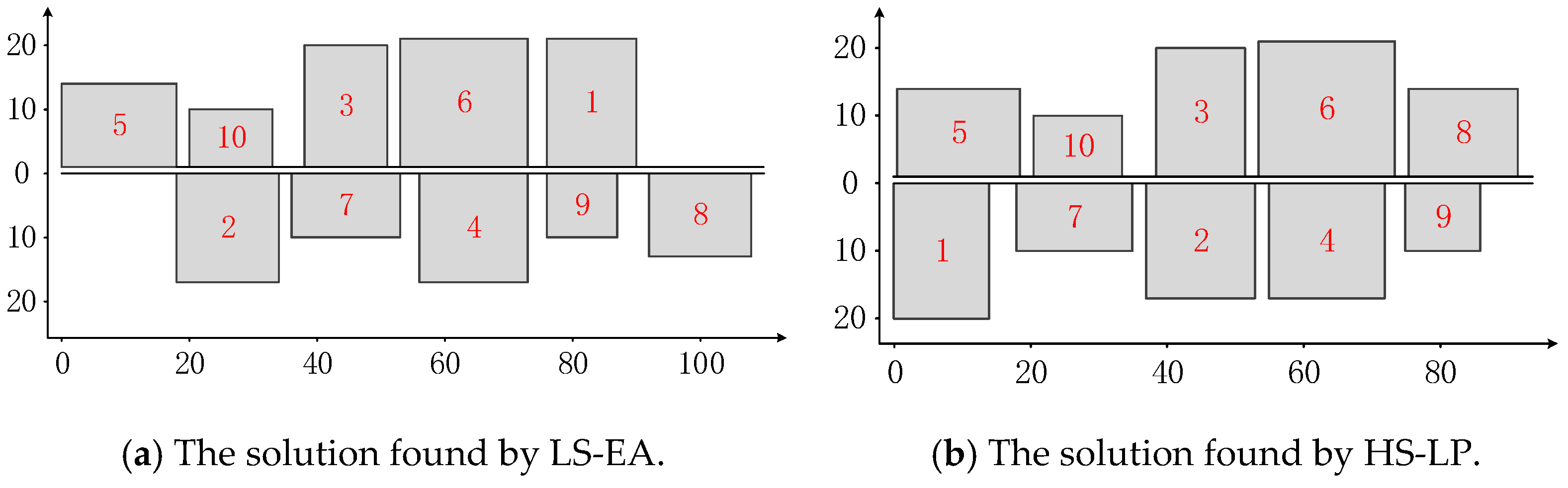
5.3. Experimental Results and Analysis

The effectiveness of the surrogate model. A set of experiments are designed to evaluate the surrogate model. The expected value of the product demand is given by a fixed interval, E(Dcp) [50, 60] and ten large variance intervals of the product demand are given, Var(Dcp) {[1, 20], [20, 50], [50, 100], [100, 200], [200, 500], [500, 1000], [1000, 2000], [2000, 5000], [5000, 10,000], [10,000, 100,000]}. For each combination of expected value interval and variance interval, 30 problem instances are randomly generated. Then, for each problem instance, randomly generate 10,000 layouts (solutions) and calculate their real objective function value (MHC) by Equation (1), the objective function value based on Naslund’s approximation method ( M H C ) by Equation (14), the value of square root term F1 by Equation (13) and linear Manhattan distance F2 by Equation (15). The top 8000 layouts are used as the training set and the remaining 2000 layouts as the test set. Each element in the training set has a pair of F1 and F2 values and MATLAB toolbox is employed to learn the coefficients a and b in Equation (16). Using a and b (the surrogate model), the fitting objective function values ( M H C ) of each element in the test set are calculated by Equation (17). Based on the test set, the mean absolute percentage error (MAPE) [37] of Naslund’s approximation and surrogate model are calculated by Equation (18). The average MAPE value of all the 30 problem instances is shown in Figure 5.
M A P E = 1 K k K | G k G k | G k × 100 % ,
where G k is the fitting objective function value ( M H C or M H C ) of the kth layout; K = 2000 is the number of layouts in the test set; and Gk is the real objective function value (MHC) of the kth layout.
It can be seen that when the expected value interval is fixed, as the variance interval increases, MAPEs of both Naslund’s approximation and the surrogate model increase. The average values of MAPEs of the surrogate model are obviously lower than those of Naslund’s approximation. Even when the value of variance is much larger than expected value, Var(Dcp) [10,000, 100,000], the surrogate model still maintains a lower average value of MAPE (0.62%).
Comparation with other approaches. LS-EA and HS-LP are independently performed for 20 runs for each problem instance with the parameter settings in Section 5.2. Table 3 presents the minimal and average material handling cost, and average runtime over the 20 runs. The material handling cost, runtime and optimality gap of EM are also provided in Table 3. The best results are highlighted in boldface.
For problem instance P8, it only takes a short time for EM to obtain a feasible solution. Although we cannot guarantee that this solution is the optimal one, it is very close to the optimal, since the average value of MAPE of the surrogate model is very small. Each run of LS-EA achieves the same solution as found by EM. This solution is represented in Figure 6a. We take P8 as an example to illustrate its decision variables. Machines 7, 5, 2, 8 and 3 are placed on row 1, thus the values of q71, q51, q21, q81 and q31 are equal to 1 and sij = 1, where i , j { 7 , 5 , 2 , 8 , 3 } and i j . The remaining machines 6, 1 and 4 are on row 2, such that q62 = q12 = q42 = 1 and sij = 1 where i , j { 6 , 1 , 4 } and i j . Machine 7 is located to the left of machines 5, 2, 8 and 3 on row 1, such that z7i1 equals to 1, where i { 5 , 2 , 8 , 3 } . Similarly, z5i1 = 1 ( i { 2 , 8 , 3 } ), z2i1 = 1 ( i { 8 , 3 } ), z831 = 1, z6i2 = 1 ( i { 1 , 4 } ) and z142 = 1. The abscissas of the pick-up point of all machines are x1 = 30, x2 = 30, x3 = 63, x4 = 52.5, x5 = 18, x6 = 8.5, x7 = 5.5, and x8 = 42. Values of other decision variables are all zero.
As the problem size increases, the computational time required for EM increases greatly. The EM can only find the optimal solutions of LP2 for P8 and P10. For other problem instances, the EM is able to find the feasible solutions within the given runtime. With the increase of scale of problem instances, LS-EA and HS-LP have significant advantages over EM. Although HS-LP is given longer runtime than LS-EA, LS-EA outperforms HS-LP in terms of average material handling cost on all problem instances except for P8. The best solutions (layouts) found by LS-EA for all problem instances are shown in Figure 6.
From Table 3, we can see that, compared with HS-LP, LS-EA reduces the minimum material handling cost most for P10 (reduces by 3.1%). The reason may be that a large offset is required by the best solution of P10. In each iteration of HS-LP, the value of offset is changed by adding a random number in {−0.5, 0, 0.5} to the current value of the offset. This local search strategy may lead to the local optima. That is, if the material handling cost of the current solution is not reduced after the offset value is added (or subtracted) by 0.5, a larger (or smaller) offset value is not considered.
To verify this speculation, the maxO in LS-EA is set to 20 to make LS-EA experience a larger runtime. MAX_k in HS-LP is set to 30 to ensure that ITER and MAX_k have similar values. Table 4 presents experimental results of LS-EA and HS_LP for problem instance P10. LS-EA can find the same solution as EM in each run when giving a larger maxO value. However, HS-LP cannot improve the solution quality under longer runtime. Figure 7 shows the best solution found by LS-EA and HS-LP for P10. We can see that the offset of the solution obtained by HS-LP is much smaller than that of LS-EA. This means that for some specific problem instances whose optimal solutions have large offsets, LS-EA can find a much better solution than HS-LP by setting a suitable value of maxO.
The effect of EA in LS-EA. For each problem instance, LS is performed to find a solution, where only the machine sequences on two rows and the extra clearance of the leftmost machine on row 1 are optimized. The extra clearance of all machines in the solution are further optimized by EA. Table 5 shows the maximum and average material handling cost reduction of solutions obtained by EA, and the average runtime of EA. We can see that the maximum reduction on material handling cost by EA is from 0.14% to 6.18% while the runtime of EA is tiny, ranging from 0.004 s to 0.837 s.

5.4. Statistical Significance

To evaluate whether there is a significant advantage of LS-EA compared to HS-LP, the nonparametric statistical tests, Sign test and Wilcoxon signed ranks test are performed. The null hypothesis is defined so that the performance of LS-EA and HS-LP shows no difference and the statistical significance level is set to 0.05. In the experiment shown in Table 3, LE-EA and HS-LP obtain 120 solutions for all six problem instances. Based on the material handling cost of these solutions, the p-values of Sign test and Wilcoxon signed ranks test are calculated by a statistical software, SPSS. The results of two tests are summarized in Table 6. It can be seen that the LS-EA has more Wins than HS-LP and both of the p-values of two tests are less than the significance level (0.05). This means that the null-hypothesis is rejected and LS-EA significantly outperforms HS-LP.

6. Conclusions

In this paper, we study an extended DRLP, where the produce demands are independent and normally distributed random variables with known expected value and variance, termed as SR-DRLP. A MIP for SR-DRLP is established. To linearize the nonlinear term in the MIP, a surrogate model is used to replace the nonlinear term to make the MIP become a mixed integer linear programming model. A high-quality solution to problem instances with no more than ten machines can be obtained by solving the linear programming model by an exact approach. A two-stage hybrid approach combining a local search and an exact approach (LS-EA) is proposed to solve large-scale problem instances. First, the LS is employed to optimize the machine sequences on two rows and the extra clearance of the leftmost machine on row 1. Then, the EA is utilized to determine the optimal extra clearances of all machines.
Experimental results show that the average absolute percentage error of the surrogate model is much smaller than that of Naslund’s approximation. LS-EA can find the same solution as EM for small-scale instances and LS-EA significantly outperforms HS-LP. Specifically, for problem instances whose optimal solutions require larger offset values, LS-EA can obtain solutions much better than HS-LP.
Future research directions include considering more optimization objectives (e.g., layout area and closeness of facilities) and extending the SR-DRLP to a stochastic robust multi-row layout problem.

Author Contributions

Conceptualization, X.W. and X.-Q.Z.; methodology, X.W. and X.-Q.Z.; software, X.W.; validation, X.W., X.-Q.Z. and X.-C.Z.; formal analysis, X.W. and X.-Q.Z.; investigation, X.W. and X.-Q.Z.; writing—original draft preparation, X.W.; writing—review and editing, X.-Q.Z.; visualization, X.W.; supervision, X.-Q.Z. and X.-C.Z.; funding acquisition, X.-Q.Z. and X.-C.Z. All authors have read and agreed to the published version of the manuscript.

Funding

This research was funded by National Natural Science Foundation of China under Grants 61873040 and 61973042, and Beijing Natural Science Foundation under Grant 1202020, and BUPT Excellent Ph.D. Students Foundation.

Institutional Review Board Statement

Not applicable.

Informed Consent Statement

Not applicable.

Data Availability Statement

Not applicable.

Conflicts of Interest

The authors declare no conflict of interest.

References

  1. Palubeckis, G. An approach integrating simulated annealing and variable neighborhood search for the bidirectional loop layout problem. Mathematics 2021, 9, 5. [Google Scholar] [CrossRef]
  2. Akturk, M.; Gultekin, H.; Karasan, O.E. Robotic cell scheduling with operational flexibility. Discret. Appl. Math. 2005, 145, 334–348. [Google Scholar] [CrossRef] [Green Version]
  3. Anjos, M.F.; Vieira, M.V.C. Mathematical optimization approach for facility layout on several rows. Optim. Lett. 2021, 15, 9–23. [Google Scholar] [CrossRef]
  4. Zuo, X.; Murray, C.C.; Smith, A.E. Solving an extended double row layout problem using multiobjective tabu search and linear programming. IEEE Trans. Autom. Sci. Eng. 2014, 11, 1122–1132. [Google Scholar] [CrossRef]
  5. Chung, J.; Tanchoco, J. The double row layout problem. Int. J. Prod. Res. 2010, 48, 709–727. [Google Scholar] [CrossRef]
  6. Wang, S.; Zuo, X.; Liu, X.; Zhao, X.; Li, J. Solving dynamic double row layout problem via combining simulated annealing and mathematical programming. Appl. Soft Comput. 2015, 37, 303–310. [Google Scholar] [CrossRef]
  7. Tang, L.; Zuo, X.; Wang, C.; Zhao, X. A MOEA/D based approach for solving robust double row layout problem. In IEEE Congress on Evolutionary Computation (CEC); IEEE: Sendai, Japan, 2015; pp. 1966–1973. [Google Scholar]
  8. Asl, A.D.; Wong, K.Y.; Tiwari, M.K. Unequal-area stochastic facility layout problems: Solutions using improved covariance matrix adaptation evolution strategy, particle swarm optimisation, and genetic algorithm. Int. J. Prod. Res. 2016, 54, 799–823. [Google Scholar]
  9. Tayal, A.; Gunasekaran, A.; Singh, S.P.; Dubey, R.; Papadopoulos, T. Formulating and solving sustainable stochastic dynamic facility layout problem: A key to sustainable operations. Ann. Oper. Res. 2017, 253, 621–655. [Google Scholar] [CrossRef] [Green Version]
  10. Kim, M.; Chae, J. Monarch butterfly optimization for facility layout design based on a single loop material handling path. Mathematics 2019, 7, 154. [Google Scholar] [CrossRef] [Green Version]
  11. Drira, A.; Pierreval, H.; Hajri-Gabouj, S. Facility layout problems: A survey. Annu. Rev. Control. 2007, 31, 255–267. [Google Scholar] [CrossRef]
  12. Hosseini-Nasab, H.; Fereidouni, S.; Fatemi Ghomi, S.M.T.; Fakhrzad, M.B. Classification of facility layout problems: A review study. Int. J. Adv. Manuf. Technol. 2018, 94, 957–977. [Google Scholar] [CrossRef]
  13. Zhang, Z.; Murray, C.C. A corrected formulation for the double row layout problem. Int. J. Prod. Res. 2012, 50, 4220–4223. [Google Scholar] [CrossRef]
  14. Amaral, A.R.S. Optimal solutions for the double row layout problem. Optim. Lett. 2013, 7, 407–413. [Google Scholar] [CrossRef]
  15. Secchin, L.D.; Amaral, A.R.S. An improved mixed-integer programming model for the double row layout of facilities. Optim. Lett. 2019, 13, 193–199. [Google Scholar] [CrossRef]
  16. Chae, J.; Regan, A.C. A mixed integer programming model for a double row layout problem. Comput. Ind. Eng. 2020, 140, 106244. [Google Scholar] [CrossRef]
  17. Amaral, A.R.S. A mixed-integer programming formulation for the double row layout of machines in manufacturing systems. Int. J. Prod. Res. 2019, 57, 34–47. [Google Scholar] [CrossRef]
  18. Dahlbeck, M.; Fischer, A.; Fischer, F. Decorous combinatorial lower bounds for row layout problems. Eur. J. Oper. Res. 2020, 286, 929–944. [Google Scholar] [CrossRef]
  19. Amaral, A.R.S. A mixed-integer programming formulation of the double row layout problem based on a linear extension of a partial order. Optim. Lett. 2021, 15, 1407–1423. [Google Scholar] [CrossRef]
  20. Güļsen, M.; Murray, C.C.; Smith, A.E. Double-row facility layout with replicate machines and split flows. Comput. Oper. Res. 2019, 108, 20–32. [Google Scholar] [CrossRef]
  21. Guan, J.; Lin, G.; Feng, H.B.; Ruan, Z.Q. A decomposition-based algorithm for the double row layout problem. Appl. Math. Model. 2020, 77, 963–979. [Google Scholar] [CrossRef]
  22. Murray, C.C.; Smith, A.E.; Zhang, Z. An efficient local search heuristic for the double row layout problem with asymmetric material flow. Int. J. Prod. Res. 2013, 51, 6129–6139. [Google Scholar] [CrossRef]
  23. Amaral, A.R.S. A heuristic approach for the double row layout problem. Ann. Oper. Res. 2020. [Google Scholar] [CrossRef]
  24. Amaral, A.R.S. A parallel ordering problem in facilities layout. Comput. Oper. Res. 2013, 40, 2930–2939. [Google Scholar] [CrossRef]
  25. Yang, X.; Cheng, W.; Smith, A.E.; Amaral, A.R.S. An improved model for the parallel row ordering problem. J. Oper. Res. Soc. 2020, 71, 475–490. [Google Scholar] [CrossRef]
  26. Gong, J.; Zhang, Z.; Liu, J.; Guan, C.; Liu, S. Hybrid algorithm of harmony search for dynamic parallel row ordering problem. J. Manuf. Syst. 2021, 58, 159–175. [Google Scholar] [CrossRef]
  27. Amaral, A.R.S. The corridor allocation problem. Comput. Oper. Res. 2012, 39, 3325–3330. [Google Scholar] [CrossRef]
  28. Ahonen, H.; de Alvarenga, A.; Amaral, A.R.S. Simulated annealing and tabu search approaches for the Corridor Allocation Problem. Eur. J. Oper. Res. 2014, 232, 221–233. [Google Scholar] [CrossRef]
  29. Kalita, Z.; Datta, D. Solving the bi-objective corridor allocation problem using a permutation-based genetic algorithm. Comput. Oper. Res. 2014, 52, 123–134. [Google Scholar]
  30. Kalita, Z.; Datta, D.; Palubeckis, G. Bi-objective corridor allocation problem using a permutation-based genetic algorithm hybridized with a local search technique. Soft Comput. 2019, 23, 961–986. [Google Scholar] [CrossRef]
  31. Zhang, Z.; Mao, L.; Guan, C.; Zhu, L.; Wang, Y. An improved scatter search algorithm for the corridor allocation problem considering corridor width. Soft Comput. 2020, 24, 461–481. [Google Scholar] [CrossRef]
  32. Fischer, A.; Fischer, F.; Hungerländer, P. A new exact approach to the space-free double row layout problem. In Operations Research Proceedings 2015; Springer International Publishing: Cham, Denmark, 2017; pp. 125–130. [Google Scholar]
  33. Palubeckis, G. Fast local search for single row facility layout. Eur. J. Oper. Res. 2015, 246, 800–814. [Google Scholar] [CrossRef]
  34. Allahyari, M.Z.; Azab, A. Mathematical modeling and multi-start search simulated annealing for unequal-area facility layout problem. Expert Syst. Appl. 2018, 91, 46–62. [Google Scholar] [CrossRef]
  35. Bozorgi, N.; Abedzadeh, M.; Zeinali, M. Tabu search heuristic for efficiency of dynamic facility layout problem. Int. J. Adv. Manuf. Technol. 2015, 77, 689–703. [Google Scholar] [CrossRef]
  36. Tavakkoli-Moghaddam, R.; Javadian, N.; Javadi, B.; Safaei, N. Design of a facility layout problem in cellular manufacturing systems with stochastic demands. Appl. Math. Comput. 2007, 184, 721–728. [Google Scholar] [CrossRef]
  37. Zhang, S.Q.; Lin, K.P. Short-term traffic flow forecasting based on data-driven model. Mathematics 2020, 8, 152. [Google Scholar] [CrossRef] [Green Version]
Figure 1. A layout for SR-DRLP.
Mathematics 09 01711 g001
Figure 2. Four symmetry layouts with the same material handling cost.
Mathematics 09 01711 g002
Figure 3. The decoding process for a coding (π = {1, 2, 3, 4, 5, 6}, b = 3, o = 2).
Mathematics 09 01711 g003
Figure 4. The relationship of Euclidean distance (F1) and Manhattan distance (F2) for the formulation of SR-DRLP.
Mathematics 09 01711 g004
Figure 5. The comparison of Naslund’s approximation and surrogate model.
Mathematics 09 01711 g005
Figure 6. The best solutions found by LS-EA for all problem instances.
Mathematics 09 01711 g006
Figure 7. The best solution found by LS-EA with larger maxO and HS-LP with larger runtime for P10.
Mathematics 09 01711 g007
Table 1. Decision variables.
Decision VariablesVariable Descriptions
xiContinuous decision variable denotes the abscissa of machine i M .
v i j + , v i j Auxiliary continuous decision variables are utilized to determine the distance between machines i M and j M \ { i } .
qirBinary variable, such that qir = 1 if machines i M is placed on the row r, otherwise qir = 0.
sijBinary variable, such that sij = 1 if both machines i M and j M \ { i } are placed on the same row, otherwise sij = 0.
zijrBinary variable, such that zijr = 1 if both machines i M and j M \ { i } are placed on the same row r R and i is placed to the left of j, otherwise zijr = 0.
Table 2. The parameters of problem instances.
Problem InstancesE(Dcp)Var(Dcp)mtl
P8(30–60)(1–20)846
P10(50–80)(50–100)1057
P15(60–100)(100–1000)1569
P20(100–200)(500–1000)20812
P30(200–500)(1000–5000)301220
P50(500–1000)(5000–10,000)501530
Table 3. Results of all problem instances.
Problem InstancesP8P10P15P20P30P50
HS-LPMin cost6.824 × 1041.608 × 1059.817 × 1055.167 × 1067.790 × 1077.188 × 108
Aver cost6.824 × 1041.608 × 1059.913 × 1055.239 × 1067.888 × 1077.299 × 108
Time (s)0.551.335.0215.4279.74519.58
LS-EAMin cost6.824 × 1041.558 × 1059.817 × 1055.164 × 1067.747 × 1077.096 × 108
Aver cost6.824 × 1041.593 × 1059.851 × 1055.208 × 1067.864 × 1077.256 × 108
Time (s) 0.521.154.9815.1776.75495.58
EMCost6.824 × 1041.483 × 1059.878 × 1055.668 × 1069.144 × 1079.578 × 108
Time (s)0.633.283600.003600.003600.003600.00
Optimality gap (%)0.000.0050.6778.0591.2598.34
Table 4. Results of problem instance P10.
Problem InstanceLS-EAHS-LPEM
Min CostAver CostTime (s)Min CostAver CostTime (s)CostTime (s)
P101.483 × 1051.483 × 1056.881.608 × 1051.608 × 1057.131.483 × 1053.28
Table 5. The maximal and average of the reduction and average runtime of EA.
Problem InstancesP8P10P15P20P30P50
Max reduction0.69%6.18%0.19%0.42%0.55%0.14%
Aver reduction0.29%2.07%0.05%0.12%0.11%0.04%
Time (s)0.0040.0040.0130.0300.1590.837
Table 6. Statistical comparison of LS-EA and HS-LP.
LS-EA versus HS-LPSign Test (p-Value)Wilcoxon Signed Ranks Test (p-Value)
Wins EqualsLoses
5639250.0080.001
Publisher’s Note: MDPI stays neutral with regard to jurisdictional claims in published maps and institutional affiliations.

