Calibrating the CreditRisk⁺ Model at Different Time Scales and in Presence of Temporal Autocorrelation †

Abstract

The CreditRisk${}^{+}$ model is one of the industry standards for the valuation of default risk in credit loans portfolios. The calibration of CreditRisk${}^{+}$ requires, inter alia, the specification of the parameters describing the structure of dependence among default events. This work addresses the calibration of these parameters. In particular, we study the dependence of the calibration procedure on the sampling period of the default rate time series, that might be different from the time horizon onto which the model is used for forecasting, as it is often the case in real life applications. The case of autocorrelated time series and the role of the statistical error as a function of the time series period are also discussed. The findings of the proposed calibration technique are illustrated with the support of an application to real data.

1. Introduction

While the development of modern portfolio credit risk models started in the 1980–1990 decade [1] within the framework of the Basel Accords, it is with the great credit crisis of 2008 [2] that increasing attention started to be paid to the precise determination of the structure of dependence among default events. It is well established [3] that tails of the distribution of the value of asset/liabilities portfolios are dominated by the structure of dependence rather than by the other fundamental components of credit risk (i.e., the marginal probability and the severity associated with each future default event). The vast research interest in modeling the structure of dependence resulted in the formalization of the so-called copula theory [4,5]. This “language” was explicitly adopted by the second generation of portfolio credit models to describe the dependence among loss events [6,7,8,9].

In this regard, the calibration issues raised by a particular structure of dependence (or, equivalently, the corresponding copula) can be as important as the choice of the structure itself. Generally, calibrating the dependence structure of a portfolio model is a demanding task, given the large number of parameters needed to provide a realistic description of the modeled dependencies, and considering that, on the other hand, historical data are usually not numerous enough to fill the sample space in a way sufficient for a precise estimation of the parameters.

In this work, we address a typical real-life problem: how to choose the frequency of the historical time series of default used to calibrate a classic credit portfolio model, CreditRisk${}^{+}$, in order to provide the most accurate estimation of the structure of dependence parameters, or, in other words, how the calibration error “scales” with the time series frequency. This problem is especially relevant for all the cases when the debtors underlying a credit portfolio are small/medium enterprises. The lack of market information, such as CDS spread, stock price, or bond yield, forces to calibrate the model using a reduced-form approach based on historical cluster data, such as default rate time series associated with the economic sector of each debtor. This case is typical in activities such as credit insurance, surety, and factoring. In most cases, publicly available time series have a sampling period ranging from one to three months (e.g., [10]), while the calibrated CreditRisk${}^{+}$ model is used on a projection horizon that is at least one year long (e.g., the unwind period required to quantify a capital requirement both in Solvency 2 and in Basel 3 regulatory frameworks).

CreditRisk${}^{+}$[11], disclosed in 1997, belongs to the first generation of portfolio credit risk models of “actuarial inspiration”. Applications of CreditRisk${}^{+}$ to the credit insurance sector are documented in the literature well before the 2008 financial credit crisis [12,13], while research activity is still ongoing in the area of actuarial science [14]. At present, CreditRisk${}^{+}$ is still one of the financial and actuarial industry standards for the assessment of credit risk in portfolios of financial loans or credit/suretyship policies.

Despite the vast research activity on this model and its calibration, the issue of using two different time scales for calibration and projection remains not investigated to date. The research conducted to date on the calibration of CreditRisk${}^{+}$ [14] has addressed the issues related to the decomposition of a given covariance matrix among the time series, which is the final necessary step to complete the calibration of the model. However, the covariance matrix is obtained by the “classical” estimator, under the assumption that the sampling period of the time series and the projection horizon are equal.

This work shows that calibrating the model at a shorter time scale than the projection horizon is possible, nontrivial, and convenient. The internal consistency of the CreditRisk${}^{+}$ assumptions when simultaneously imposed at different time scales has been proved and guarantees that the investigated calibration mode is not ill-posed. However, the form of the covariance estimator needed to obtain a set of parameters coherent with a specific projection horizon, using time series with a smaller sampling period, depends on the two chosen time scales. Indeed, the proposed estimator coincides with the classical one only when calibration and projection time scales are equal. Finally, we show that calibrating at a smaller time scale than the projection one provides a more precise estimation of the model parameters. The estimation error and its dependence on the difference between the two time scales are discussed.

The article is organized as follows. In Section 2, we summarize assumptions and features of the CreditRisk${}^{+}$ model. In Section 3, we discuss the internal consistency of the model assumptions when imposing them to be simultaneously true at different time horizons. The calibration of the model parameters, which define the dependence structure, is considered in Section 4. The different degree of precision of the estimators defined at increasing time scales is discussed in Section 5. The techniques introduced in this work are applied to a real-world case study in Section 6. The main results are summarized in Section 7.

2. The CreditRisk⁺ Model

The CreditRisk${}^{+}$ model is a portfolio model developed by Credit Suisse First Boston (CSFB) by Tom Wilde [15] and coworkers, first documented in [11] and later widely discussed in [16]. It is a model actuarially inspired in the sense that losses are due only to default events and not to other sources of financial risk, e.g., variation of the credit standing (the so-called “credit migration” effect). CreditRisk${}^{+}$ can be classified as a frequency–severity model, cast in a single-period framework, with the peculiarity that a doubly-stochastic process (i.e., the Poisson–Gamma mixture) describes the frequency of default events. Loss severity is assumed to be deterministic, although this ansatz can be easily relaxed at the cost of some additional computational burden. However, severity-related issues can be neglected for what follows.

The structure of dependence of default events is described using a factor model framework, where factors are unobservable (i.e., latent) stochastic “market” variables, whose precise financial/actuarial identification is irrelevant since the model integrates on all possible realizations (“market scenarios”). Therefore, CreditRisk${}^{+}$ can be further classified into the family of factor models and, in particular, into the subfamily of conditionally independent factor models, since, conditionally on the values assumed by the factors, defaults are supposed (by the model) to be independent.

The structure of the model can be summarized as follows. Let N be the number of different risks in a given portfolio and ${1\mathrm{I}}_i$ the default indicator function of the i-th risk ($i=1,\dots ,N$) over the time horizon $(t,T]$. The indicator function ${1\mathrm{I}}_i$ is a Bernoulli random variable such that

$$\mathbf{E}\left[{1\mathrm{I}}_i\right]\hspace{0.17em}=\hspace{0.17em}{q}_i,\mathbf{var}\left[{1\mathrm{I}}_i\right]\hspace{0.17em}=\hspace{0.17em}{q}_i(1-q_i),i=1,\dots ,N.$$

(1)

The “portfolio loss” L over the reference time horizon $(t,T)$ is then given by

$$L=\sum _{i=1}^N{1\mathrm{I}}_i{E}_i$$

(2)

where each exposure $E_i$ is supposed to be deterministic.

In order to ease the semianalytic computation of the distribution of L, the model introduces a new set of variables $Y_i$, each replacing the corresponding indicator function ${1\mathrm{I}}_i$ ($i=1,\dots ,N$). The new variables $Y_i$ are supposed to be Poisson-distributed, conditionally on the value assumed by the market latent variables.

Assumption 1

(CreditRisk${}^{+}$ distributional assumption). Given a time horizon $(t,T]$ and a set of N risky debtors, the number $Y_i$ of insolvency events generated by each i-th debtor over $(t,T]$ is distributed as follows:

$$Y_i\sim \mathrm{Poisson}\left(p_i(\mathbf{\Gamma })\right),p_i(\mathbf{\Gamma }):=q_i·\left({\omega }_{i0}+\sum _{k=1}^K{\omega }_{ik}{\Gamma }_k\right)$$

(3)

where $\mathbf{\Gamma }=({\Gamma }_1\dots {\Gamma }_K)\in {\mathbb{R}}_{+}^K$ is an array of independent r.v.’s such that

$${\Gamma }_k\sim \mathrm{Gamma}\left({\beta }_k^{-1},{\beta }_k\right),{\beta }_k\in {\mathbb{R}}_{+}$$

(4)

and the factor loadings ${\omega }_{ik}$ are supposed to be all non-negative and to sum up to unity:

$$\begin{array}{c}{\omega }_{ik}\ge 0,\hspace{1em}\hspace{1em}i=1,\dots ,N,k=0,\dots ,K,\hfill \\ {\displaystyle \sum _{k=0}^K{\omega }_{ik}=1,}\hspace{1em}i=1,\dots ,N.\hfill \end{array}$$

(5)

The $\mathbf{\Gamma }$ parameters set $\{{\beta }_1\dots {\beta }_K\}$ is equivalent to the classical shape-scale parameterization $\{{\alpha }_k,{\beta }_k\}$ of each Gamma distributed r.v. ${\Gamma }_k$, after having imposed the assumption $\mathbf{E}\left[{\Gamma }_k\right]\hspace{0.17em}=\hspace{0.17em}1$, that is stated in the original formulation of the CreditRisk${}^{+}$ model. Hence, the k-th scale parameter ${\beta }_k$ is equal to the variance ${\sigma }_k^2$ of ${\Gamma }_k$. Given the independence among ${\Gamma }_k$’s, the covariance matrix $\Sigma$ takes the form

$$\Sigma :=\mathbf{cov}\left[\mathbf{\Gamma }\right]\hspace{0.17em}=\hspace{0.17em}\mathbf{diag}\left({\sigma }_1^2\dots {\sigma }_K^2\right)\hspace{0.17em}=\hspace{0.17em}\mathbf{diag}\left({\beta }_1\dots {\beta }_K\right)$$

(6)

Assumption 1 implies that $q_i$ is the unconditional expected default frequency

$$q_i=\mathbf{E}\left[p_i(\mathbf{\Gamma })\right]\hspace{0.17em}=\hspace{0.17em}{\int }_{{\mathbb{R}}_{+}^K}{p}_i(\mathbf{\Gamma })f\left(\mathbf{\Gamma }\right)d{\Gamma }_1\dots d{\Gamma }_k,$$

(7)

where

$$f\left(\mathit{x}\right)\hspace{0.17em}=\hspace{0.17em}\prod _{k=1}^K{\displaystyle \frac{x_k^{{\alpha }_k-1}}{{\beta }_k^{{\alpha }_k}\Gamma \left({\alpha }_k\right)}}{e}^{-x_k/{\beta }_k},x_k\ge 0,{\alpha }_k,{\beta }_k>0,$$

(8)

and that the identity between the expected values of the original Bernoulli variable ${1\mathrm{I}}_i$ and the new Poisson variable $Y_i$ is granted:

$$\mathbf{E}\left[Y_i\right]\hspace{0.17em}=\hspace{0.17em}\mathbf{E}\left[{1\mathrm{I}}_i\right]\hspace{0.17em}=\hspace{0.17em}{q}_i.$$

(9)

The portfolio loss is now represented by the r.v. $L_{\mathrm{Y}}$

$$L_{\mathrm{Y}}=\sum _{i=1}^N{Y}_i·E_i,\mathrm{where}{Y}_i|\mathbf{\Gamma }\sim \mathrm{Poisson}\left(p_i(\mathbf{\Gamma })\right).$$

(10)

In [11], the distribution of $L_{\mathrm{Y}}$ is obtained by using a recursive method, further described in [17]. The accuracy, stability, and possible variants of the original algorithm are discussed in [16]. The same distribution can be easily computed through Monte Carlo simulation due to the availability of a dedicated importance sampling algorithm in [18].

Notice that, although the distributions of L and $L_{\mathrm{Y}}$ differ, the expected value of the portfolio loss is the same $\mathbf{E}\left[L\right]\hspace{0.17em}=\hspace{0.17em}\mathbf{E}\left[L_{\mathrm{Y}}\right]$.

In the language of copula functions, the structure of dependence implied by (3) corresponds [19] to a multivariate Clayton copula, i.e., an Archimedean copula where latent variables are Gamma-distributed (for the relation between Archimedean copula functions and factor models see, e.g., ([9] [§2.1])). The copula parameters are the factor loadings ${\omega }_{ik}$ and they can be gathered, taking into account the normalization condition stated in Assumption 1, in an $N\times K$ matrix $\Omega$:

$$\Omega :=\left(\begin{array}{ccc}{\omega }_{11}& \dots & {\omega }_{1K}\\ ⋮& \ddots & ⋮\\ {\omega }_{N1}& \dots & {\omega }_{NK}\end{array}\right),$$

(11)

which is, for typical values of N and K, much smaller than the $N\times N$ covariance matrix between the default indicators $1\mathrm{I}$.

Remark 1.

This work is specifically focused on improving the estimation of the CreditRisk${}^{+}$ copula parameters $\{\Omega ,\Sigma \}$. Further investigations on the properties of CreditRisk${}^{+}$ dependence structure, apart from those needed for the estimation improvement, and its comparison with the other copulae are beyond the scope of this study.

As shown in [14], it holds

$$\mathbf{cov}\left[Y_i,Y_j\right]\hspace{0.17em}=\hspace{0.17em}{q}_i{q}_j\sum _{k=1}^K{\omega }_{ik}{\omega }_{jk}{\sigma }_k^2+{\delta }_{ij}{q}_i,$$

(12)

where ${\delta }_{ij}$ is the Kronecker delta. Equation (12) allows the calibration of the factor loadings, and thus of the dependence structure of the CreditRisk${}^{+}$ model, by matching the observed covariance matrix of historical default time series with model values. However, since the model is defined in a single-period framework, with a reference “forecasting” time horizon $(t,T]$, that is typically of 1 year, i.e., $T=t+1$, it is not a priori evident how to use historical time series with a different frequency (e.g., quarterly) in a consistent way, when calibrating the model parameters. Naively, it is reasonable to expect that the larger the information provided by the historical time series (i.e., the higher the frequency), the better the calibration. This issue is addressed in the next sections.

3. CreditRisk⁺ Using Multiple Unwind Periods

The original CreditRisk${}^{+}$ formulation, summarized in Assumption 1, defines the model in a uniperiodal framework, where only one time scale $T-t$ is considered. In this section, we discuss the internal consistency of the model assumption when imposing it more than once at distinct time scales. In this context, the expression “internal consistency” means that it is possible and well-posed imposing Assumption 1 to be true at two distinct time scales. The same applies also considering a slightly modified version of the CreditRisk${}^{+}$ framework (i.e., imposing Assumption 2, introduced in the following, instead of Assumption 1).

Extending the original CreditRisk${}^{+}$ formulation to a multiperiod framework enables the calibration of the model considering a time scale different from the one chosen for its application. The results presented in this section are applied in the next Section 4 to estimate the elements of the matrix

$$A:={\Omega }^T\Sigma \Omega .$$

(13)

Estimating A is a fundamental step in order to complete the calibration of the model. In Section 4 estimators are defined using historical series sampled with a period that is not necessarily equal to the projection horizon on which $\Sigma$ and $\Omega$ are defined. Section 5 shows the convenience of choosing a sampling period shorter than the projection horizon in order to evaluate $\widehat{A}$.

3.1. The Single Unwind Period Case

As discussed in Section 2, in CreditRisk${}^{+}$ each risk (i.e., debtor) is modeled by a Poisson distributed r.v. $Y_i$, although the Bernoulli distribution is the natural choice to represent absorbing events, such as default. Assumption 1 is convenient in terms of analytical tractability since $L_{\mathrm{Y}}$ distribution can be computed through a semianalytical method. However, in order to address the problem of calibrating CreditRisk${}^{+}$ in a “roll-over” framework, defined by an arbitrary set of time intervals, it is useful to recover the Bernoulli representation of each debtor by introducing a new r.v. ${\tilde{Y}}_i:={1\mathrm{I}}_{Y_i>0}$.

Both the r.v. $Y_i$ and its distribution parameter $p_i(\mathbf{\Gamma })$ can take values larger than 1. This is formally correct, given that $Y_i\sim \mathrm{Poisson}\left(p_i(\mathbf{\Gamma })\right)$, despite not coping with the representation of absorbing events, that can occur at most once by definition. The so-called “Poisson approximation”, introduced by substituting ${1\mathrm{I}}_i$ with $Y_i$, is numerically sound as $q_i$ approaches to zero—a condition that is well fulfilled in most real world relevant cases.

Indeed, Assumption 1 implies that ${\tilde{Y}}_i|\mathbf{\Gamma }\sim \mathrm{Bernoulli}\left({\tilde{p}}_i(\mathbf{\Gamma })\right)$ where the distribution parameter is

$${\tilde{p}}_i(\mathbf{\Gamma })=\mathrm{Prob}(Y_i>0|\mathbf{\Gamma })=1-exp\left[-q_i\left({\omega }_{i0}+\sum _{k=1}^K{\omega }_{ik}{\Gamma }_k\right)\right].$$

(14)

It holds by construction

$$\mathbf{E}\left[{\tilde{Y}}_i\right]\hspace{0.17em}=\hspace{0.17em}{\int }_{{\mathbb{R}}_{+}^K}{\tilde{p}}_i(\mathbf{\Gamma })f(\mathbf{\Gamma })d{\Gamma }_1\dots d{\Gamma }_K.$$

(15)

Computing the integral in (15) and then approximating the term $exp[-q_i{\omega }_0]$ with its second order Taylor series centered at $q_i=0$ leads to the following result.

Proposition 1

(Asymptotic equivalence between Bernoulli and Poisson representation of risks). Let ${\tilde{Y}}_i:={1\mathrm{I}}_{Y_i>0}$ where $Y_i$ is distributed according to Assumption 1. Then

$${\tilde{q}}_i:=\mathbf{E}\left[{\tilde{Y}}_i\right]\hspace{0.17em}=\hspace{0.17em}1-e^{-q_i{\omega }_{i0}}\prod _{k=1}^K{\left(1+q_i{\omega }_{ik}{\sigma }_k^2\right)}^{-1/{\sigma }_k^2}.$$

(16)

Further,

$${\tilde{q}}_i=q_i+\mathcal{O}\left(q_i^2\right)\stackrel{q_i\to 0^{+}}{\to }{q}_i.$$

(17)

Proposition 1 implies that $\mathbf{E}\left[L_{Y_i}\right]\simeq \mathbf{E}\left[L_{{\tilde{Y}}_i}\right]$, provided that $q_i\ll 1$. Moreover, the same result enables also the exact satisfaction of $\mathbf{E}\left[L_{Y_i}\right]\hspace{0.17em}=\hspace{0.17em}\mathbf{E}\left[L_{{\tilde{Y}}_i}\right]$, in case the stochastic parameter ${\tilde{p}}_i(\mathbf{\Gamma })$ is redefined through the substitution $q_i\mapsto q_i^{\prime }$, where $q_i^{\prime }$ verifies the following modified version of (16):

$$\mathbf{E}\left[{\tilde{Y}}_i\left(q_i^{\prime }\right)\right]\hspace{0.17em}=\hspace{0.17em}1-e^{-q_i^{\prime }{\omega }_{i0}}\prod _{k=1}^K{\left(1+q_i^{\prime }{\omega }_{ik}{\sigma }_k^2\right)}^{-1/{\sigma }_k^2}=q_i=\mathbf{E}\left[Y_i\right].$$

(18)

It is worth noticing that the substitution ${1\mathrm{I}}_i\mapsto Y_i$ discussed in Section 2 implies the preservation of the expected value $\mathbf{E}\left[L\right]\hspace{0.17em}=\hspace{0.17em}\mathbf{E}\left[L_Y\right]$ due to the fact that it is done before the introduction of the market factors $\mathbf{\Gamma }$. On the other hand, restoring the Bernoulli representation of each risk after having introduced the dependence structure requires the results presented in Proposition 1.

Proposition 1 permits the introduction of a slightly modified version of the CreditRisk${}^{+}$ model that is asymptotically equivalent to the original one stated in Assumption 1. The equivalence between the two models is further analyzed in the next sections.

Assumption 2

(Modified CreditRisk${}^{+}$ distributional assumption). Given a time horizon $(t,T]$ and a set of N risky debtors, the number of insolvency events generated by each i-th debtor over $(t,T]$ is represented by the r.v. ${\tilde{Y}}_i\sim \mathrm{Bernoulli}\left({\tilde{p}}_i(\mathbf{\Gamma })\right)$, where the distribution parameter ${\tilde{p}}_i(\mathbf{\Gamma })$ satisfies (14). Assumptions on market factors Γ and factor loadings Ω remain the same stated in Assumption 1.

In Assumption 2 the linear dependence of the parameters $p_i(\mathbf{\Gamma })$ from the latent variables has been replaced with a log link function. Thus, the modified version of CreditRisk${}^{+}$ is also referred to as “exponential” in the following.

3.2. The Multiple Unwind Periods Case

This section investigates the consequences of imposing the internal consistency of Assumption 1 or Assumption 2 at distinct time scales. Assumptions 3 and 4 are introduced hereinafter, in order to specify the family of parameters that have to be considered at the distinct time intervals where the model is applied.

The following assumption guarantees the internal consistency at different time scales of the classical CreditRisk${}^{+}$ model, defined in Assumption 1.

Assumption 3

(CreditRisk${}^{+}$ parameters at different time scales). Let $t\equiv t_0,t_1,\dots ,t_m\equiv T$ be a partition of the time interval $(t,T]$. Let Assumption 1 be satisfied over each j-th interval $(t_{j-1},t_j]$ by the set $\left\{Y_i^{\left(j\right)}\right\}$ ($i=1\dots N$), where $Y_i^{\left(j\right)}$ is the r.v. representing the i-th risk observed during the j-th interval and the following holds for the associated set $\{q_i^{\left(j\right)};{\mathbf{\Gamma }}^{\left(j\right)};{\Omega }^{\left(j\right)}\}$ of parameters and market factors:

$$q_i^{\left(j\right)}\hspace{1em}=\hspace{1em}{q}_i\frac{t_j-t_{j-1}}{T-t}=\mathrm{constant},$$

(19)

$${\Gamma }_k^{\left(j\right)}\hspace{1em}\sim \hspace{1em}\mathrm{Gamma}\left({\displaystyle {\sigma }_k^{-2}{\xi }_{kj}^{-1}\frac{t_j-t_{j-1}}{T-t},{\sigma }_k^2{\xi }_{kj}\frac{T-t}{t_j-t_{j-1}}}\right),$$

(20)

$${\Omega }^{\left(j\right)}\hspace{1em}=\hspace{1em}\Omega ,$$

(21)

where ${\xi }_{kj}\in {\mathbb{R}}_{+}$.

Further, the following assumption guarantees the internal consistency at different time scales of the modified version of CreditRisk${}^{+}$ model, introduced in Assumption 2.

Assumption 4

(Modified CreditRisk${}^{+}$ parameters at different time scales). Let $t\equiv t_0,t_1,\dots ,t_m\equiv T$ be a partition of the time interval $(t,T]$. Let Assumption 2 be satisfied over each j-th interval $(t_{j-1},t_j]$ by the set $\left\{{\tilde{Y}}_i^{\left(j\right)}\right\}$ ($i=1\dots N$), where ${\tilde{Y}}_i^{\left(j\right)}$ is the r.v. representing the i-th risk observed during the j-th interval. The associated set $\{q_i^{\left(j\right)};{\mathbf{\Gamma }}^{\left(j\right)};{\Omega }^{\left(j\right)}\}$ of parameters and market factors satisfies the same assumptions stated in Assumption 3.

Finally, for the sake of simplicity, the additional Assumption 5 is introduced, with regard to the independence among market factors considered at different times. However, being possible that real-data time series violate Assumption 5, this assumption is weakened in the following Section 3.3.

Assumption 5

(Non-autocorrelated market factors). Given Assumption 3, let

$$\mathbf{cov}\left[{\Gamma }_k^{\left(j\right)},{\Gamma }_k^{\left(j^{\prime }\right)}\right]\hspace{0.17em}=\hspace{0.17em}{\delta }_{j{j}^{\prime }}\mathbf{var}\left[{\Gamma }_k^{\left(j\right)}\right].$$

(22)

Considering the assumptions introduced above, we prove that CreditRisk${}^{+}$ is internally consistent when extended to a roll-over framework.

Theorem 1

(Internal consistency of CreditRisk${}^{+}$ in absence of autocorrelation). Let us consider a set of risks $\left\{Y_i\right\}$ ($i=1\dots N$), observed through a time horizon $(t,T]$, and an arbitrary partition $t\equiv t_0,t_1,\dots ,t_m\equiv T$ of $(t,T]$, such that Assumptions 3 (“CreditRisk${}^{+}$ parameters at different time scales”) and Assumption 5 (“non-autocorrelated market factors”) are verified with

$${\xi }_{kj}=1$$

(23)

for each $i=1\dots N$, $k=1\dots K$ and $j=1\dots m$. Then $\left\{Y_i\right\}$ satisfies Assumption 1 (“CreditRisk${}^{+}$ distributional assumption”) over $(t,T]$.

The statement above remains true replacing Assumption 3 with Assumption 4 (“modified CreditRisk${}^{+}$ parameters at different time scales”) and Assumption 1 with Assumption 2 (“modified CreditRisk${}^{+}$ distributional assumption”), ceteris paribus.

The proof of Theorem 1 is reported in Appendix A.1.

This result shows that extending the CreditRisk${}^{+}$ model to a multiperiod framework is well-posed.

Remark 2.

The choice ${\xi }_{jk}=1$ implies no loss of generality, since a different (positive) constant ${\xi }_{jk}=c$ is equivalent to redefine the variances of the market factors $c{\sigma }_k^2\mapsto {\sigma }_k^2$.

3.3. Internal Consistency and Autocorrelation in Time Series

As shown in Section 2, the dynamics of each parameter $p_i$ is induced by the latent Gamma factors only. Imposing Assumption 5 to any (arbitrarily short) time scale implies that considered time series ${\left\{{\Gamma }_k^{\left(j\right)}\right\}}_{j=1,2,\dots }$ must exhibit zero autocorrelation. Hence autocorrelation must be completely absent from the historical default frequencies too.

However, this requirement could not be satisfied by the observed time series used in calibrating the model. Indeed, we need to verify that the model can preserve its internal consistency if autocorrelation has to be considered.

The purpose of this work is to investigate whether it is possible and convenient to calibrate the CreditRisk${}^{+}$ model at a time scale that copes with the available historical data (i.e., the sampling period of the historical time series) instead of using the same time scale needed for projections (usually bigger). Hence, in case it is not possible to preserve the internal consistency of the model at each arbitrary time scale, due to the presence of autocorrelation, it is sufficient to ask that it holds up to the smallest of the two time scales of interest—the historical sampling period and the projection horizon.

Let us specialize to the constant mesh case $t_j-t_{j-1}=(T-t)/m={\delta }_m$. This choice copes with a typical real case, where the sampling period ${\delta }_m$ of the available historical time series is constant and the considered projection horizon $T-t$ is a multiple of it. Under these premises, a weakened version of Assumption 5 is introduced.

Assumption 6

(Autocorrelated market factors). Given Assumption 3, for each k-th latent variable, considered at the time scale ${\delta }_m$, a time-invariant ACF ${\varrho }_{xk}$ exists, such that

$$\mathbf{cov}\left({\Gamma }_k^{\left(j\right)},{\Gamma }_k^{(j+x)}\right)\hspace{0.17em}=\hspace{0.17em}{\varrho }_{xk}\mathbf{var}\left({\Gamma }_k^{\left(j\right)}\right).$$

(24)

Furthermore, the following closure with respect to the addition holds

$$\sum _{j=1}^m{\Gamma }_k^{\left(j\right)}\sim \mathrm{Gamma}({\alpha }_k,{\beta }_k)$$

(25)

for a couple ${\alpha }_k,{\beta }_k$ of shape and scale parameters.

Assumption 6 is considered instead of Assumption 5 to state the following alternate version of Theorem 1.

Theorem 2

(Internal consistency of CreditRisk${}^{+}$ model in presence of autocorrelation). Let us consider a set of risks $\left\{Y_i\right\}$ ($i=1\dots N$), observed through a time horizon $(t,T]$, and a uniform partition ${\{t_j:=t+j{\delta }_m\}}_{j=1\dots m}$ of $(t,T]$, such that Assumption 3 (“CreditRisk${}^{+}$ parameters at different time scales”) and Assumption 6 (“autocorrelated market factors”) are verified with

$${\xi }_{kj}={\left[1+2\sum _{x=1}^{m-1}{\varrho }_{xk}\left(1-\frac{x}{m}\right)\right]}^{-\frac{1}{2}}$$

(26)

for each $i=1\dots N$, $k=1\dots K$ and $j=1\dots m$. Then $\left\{Y_i\right\}$ satisfies Assumption 1 (“CreditRisk${}^{+}$ distributional assumption”) over $(t,T]$.

The statement above remains true replacing Assumption 3 with Assumption 4 (“modified CreditRisk${}^{+}$ parameters at different time scales”) and Assumption 1 with Assumption 2 (“modified CreditRisk${}^{+}$ distributional assumption”), ceteris paribus.

The proof of Theorem 2 is reported in Appendix A.2.

Assumption 6 can be either well-posed or ill-posed, depending on the considered ${\varrho }_{xk}$. The trivial case ${\varrho }_{xk}=0$ for each $x\in \mathbb{Z}$ copes with Assumption 5. Correlated Gamma variables, as well as the distributional properties of the sum of Gamma variables, have been intensively studied in the literature, and this is still an active research field [20,21,22,23], due to its relevance for information technology. At least in case of identically distributed Gamma variables—such as ${\Gamma }_k^{\left(j\right)}$ in our framework—with ACF obeying to a power-law

$${\varrho }_{xk}={\rho }_k^{\left|x\right|},{\rho }_k\in (0,1),$$

(27)

the distribution of the sum ${\Gamma }_k$ is known to be approximately Gamma [20], while more generical cases imply the sum to be distributed differently [22,23]. Moreover, it is known that partial sums of independent Gamma variables can be used to generate sequences of (auto)correlated Gamma variables [21].

Remark 3.

The exponential ACF in Equation (27) provides a non-trivial case that satisfies Assumption Assumption 6 and, thus, Theorem 2. In the following Section 4.4, Theorem 2 permits the estimation of A in presence of autocorrelated time series. Equation (27) is then considered in Section 5.3 to investigate numerically the estimators introduced in Section 4.4. However, to date, a general framework is missing to tell whether a given ${\varrho }_{xk}$ lets the partial sums ${\sum }_j{\Gamma }_k^{\left(j\right)}$ remain (approximately) Gamma distributed, with the exception of exponential ACFs.

The estimators introduced in Section 4.4 to consider autocorrelation in time series are still applicable to an inconsistent framework, provided that at least the latent variables ${\Gamma }_k$ (defined onto the projection horizon) are Gamma distributed and ${\Gamma }_k^{\left(j\right)}$ satisfy the mean and variance requirements implied by Assumption 6 above.

4. Calibration of the Structure of Dependence

The model is calibrated based on a partition of the risks in H homogeneous sets $c_h\left(t\right)$, $h=1,\dots ,H$. In this context “homogeneity” means that two risks belonging to the same set $c_h\left(t\right)$ have the same vector of factor loadings ${\mathit{\omega }}^{\left(h\right)}$. The sets have an explicit time dependence since they can change by the occurrence of defaults. On the contrary, the structure of dependence, defined by ${\mathit{\omega }}^{\left(h\right)}$ is supposed to be time-independent.

Hence, solving the calibration problem requires the evaluation of

• H factor loading vectors ${\left\{{\mathit{\omega }}^{\left(h\right)}\right\}}_{h=1\dots H}$, that link each of the homogenous clusters to the K latent variables;
• K volatilities ${\left\{{\sigma }_k\right\}}_{k=1\dots K}$, needed to specify the distribution of each of the latent variables.

The calibration is achievable by a two-step procedure. Firstly, the matrix $A:={\Omega }^T\Sigma \Omega$, introduced in Section 3, is estimated. Then, A is decomposed under the proper constraints in order to evaluate $\Omega$ and $\Sigma$ separately. This section describes a method to complete the first step, providing an estimator of A both for the single and the multiple unwind period cases, with a moment-matching approach that allows expressing $\widehat{A}$ as a function of the covariance matrix among the historical frequencies of default. The second step is addressed later in Section 6, which provides an example of calibration using a real data set.

Adopting the standard CreditRisk${}^{+}$ Assumption 1, Equation (12) can be used to link the covariance matrix among the historical frequencies of default with the matrix A. In Section 4.1, $\widehat{A}$ is provided in the case of historical frequencies of default, sampled with the same tenor of the projection horizon. In Section 4.2, $\widehat{A}$ is generalized to the case of historical frequencies of default sampled with an arbitrary tenor.

Furthermore, in Section 4.3, $\widehat{A}$ is determined under the exponential version of the CreditRisk${}^{+}$ framework, introduced in Assumption 2. Thanks to this modified assumption, the corresponding functional form of $\widehat{A}$ is simpler than the one obtained in Section 4.2 based on Assumption 1.

Section 4.2 and Section 4.3 cope with Assumption 5, that implies absence of autocorrelation in time series. The final Section 4.4 uses Assumption 6 instead, generalizing the main results presented in this section to the case where autocorrelation must be taken into account. In this case, the simpler form of $\widehat{A}$ obtained in Section 4.3 comes in handy in the generalization to the non-trivial ACF case.

4.1. The Single Unwind Period Case

The first case considered is that of a single unwind period $(t,T]$. For each set $c_h\left(t\right)$, let $n_h\left(t\right):=\left|c_h\left(t\right)\right|$, $F_h:=\frac{1}{n_h\left(t\right)}{\sum }_{i\in c_h\left(t\right)}{Y}_i$ and $G_{h}1-F_h$. The expected values of $F_h$ and $G_h$ are respectively:

$$q_h\hspace{1em}:=\hspace{1em}\mathbf{E}\left[F_h\right]\hspace{0.17em}=\hspace{0.17em}\frac{{\sum }_{i\in c_h\left(t\right)}{q}_i}{n_h\left(t\right)},$$

(28)

$$s_h\hspace{1em}:=\hspace{1em}\mathbf{E}\left[G_h\right]\hspace{0.17em}=\hspace{0.17em}1-\mathbf{E}\left[F_h\right].$$

(29)

Remark 4.

The slight abuse of notation in (28) is done to avoid the introduction of a new symbol to represent $\mathbf{E}\left[F_h\right]$. However, the letters chosen for indexing risks and cluster (“i” and “h” respectively) are maintained in the following of this work, clarifying the meaning of the “q” symbol each time it is used.

For any pair of sets of risks $\{h,h^{\prime }\}$, the covariance between the default frequencies is:

$$\begin{array}{ccc}\hfill \mathbf{cov}\left(F_h,F_{h^{\prime }}\right)& =& \mathbf{E}\left[\left(F_h-\mathbf{E}\left[F_{h^{\prime }}\right]\right)\left(F_{h^{\prime }}-\mathbf{E}\left[F_{h^{\prime }}\right]\right)\right]\hfill \\ & =& \frac{1}{n_h{n}_{h^{\prime }}}\mathbf{E}\left[\sum _{i\in c_h}\left(Y_i-q_i\right)\sum _{i^{\prime }\in c_{h^{\prime }}}\left(Y_{i^{\prime }}-q_{i^{\prime }}\right)\right]\hfill \\ & =& \frac{1}{n_h{n}_{h^{\prime }}}\sum _{i\in c_h}\sum _{i^{\prime }\in c_{h^{\prime }}}\mathbf{cov}\left(Y_i,Y_{i^{\prime }}\right),\hfill \end{array}$$

(30)

that, using Equation (12), becomes:

$$\mathbf{cov}\left(F_h,F_{h^{\prime }}\right)\hspace{0.17em}=\hspace{0.17em}\frac{1}{n_h{n}_{h^{\prime }}}\sum _{i\in c_h}\sum _{i^{\prime }\in c_{h^{\prime }}}\left(q_i{q}_{i^{\prime }}\sum _{k=1}^K{\omega }_{ik}{\omega }_{i^{\prime }k}{\sigma }_k^2+{\delta }_{i{i}^{\prime }}{q}_i\right).$$

(31)

Equation (31) shows the relation between the observed covariance of default frequencies and the factor loadings, describing the structure of dependence of the model.

Moreover, assuming that all risks in a given homogenous set share the same factor loadings, the above expression simplifies to:

$$\mathbf{cov}\left(F_h,F_{h^{\prime }}\right)\hspace{0.17em}=\hspace{0.17em}{q}_h{q}_{h^{\prime }}\sum _{k=1}^K{\omega }_{hk}{\omega }_{h^{\prime }k}{\sigma }_k^2+{\delta }_{h{h}^{\prime }}\frac{q_h}{n_h}$$

(32)

Notice that the second term in Equation (32) is present only when $h=h^{\prime }$, and becomes quickly negligible as $n_h$ grows (since $q_h<1$).

Equation (32) enables the estimation of A over the same time scale $T-t$ used for projections:

$${\widehat{A}}_{h{h}^{\prime }}=\frac{1}{q_h{q}_{h^{\prime }}}\left[\mathbf{c}\hat{\mathbf{o}}\mathbf{v}\left(F_h,F_{h^{\prime }}\right)\hspace{0.17em}-\hspace{0.17em}{\delta }_{h{h}^{\prime }}\frac{q_h}{n_h}\right].$$

(33)

4.2. The Multiple Unwind Period Case

Let us consider a set of H time series defined using a constant step ${\delta }_m=(T-t)/m$. As done in Section 2, each variable introduced in Section 4.1 for the time interval $(t,T]$ can be redefined over each of the considered time intervals. Namely, in the following we use the set of observables quantities $\{F_h,G_h,q_h,s_h\}$, measured either over $(t,T]$ or $(t_{j-1},t_j=t_{j-1}+{\delta }_m]$ or a generic time interval $(t,t^{\prime }]$. For the latter two cases, we introduce the notation $\{F_h^{\left(j\right)},G_h^{\left(j\right)},q_h^{\left(j\right)},s_h^{\left(j\right)}\}$ and $\{F_h(t,t^{\prime }),G_h(t,t^{\prime }),\dots \}$, respectively. Further, the variables

$$F_{mh}\hspace{1em}:=\hspace{1em}1-\prod _{j=1}^m\left[1-F_h^{\left(j\right)}\right],$$

(34)

$$G_{mh}\hspace{1em}:=\hspace{1em}\prod _{j=1}^m{G}_h^{\left(j\right)}=1-F_{mh}$$

(35)

are introduced.

In CreditRisk${}^{+}$, $F_h(t,t^{\prime })$ arises from a doubly stochastic process, since each absorbing event is generated conditioned to the latent systematic factors. For the sake of simplicity, we neglect the idiosyncratic uncertainty brought by each $Y_i(t,t^{\prime })$. In fact, for $n_h\left(t\right)$ large enough, the Bernoulli (or Poisson) r.v.’s contributions to the variance of $F_h(t,t^{\prime })$ are dominated by the contribution of $\mathbf{\Gamma }(t,t^{\prime })$. This permits the following assumption.

Assumption 7

(Large clusters). For each cluster $c_h$ ($h=1\dots H$) and each time interval $(t,t^{\prime }]\subseteq (t,T]$ it holds

$$\mathbf{var}\left[F_h(t,t^{\prime })|\mathbf{\Gamma }(t,t^{\prime })\right]\hspace{0.17em}=\hspace{0.17em}0.$$

Then the following holds:

Proposition 2

(CreditRisk${}^{+}$ scale-invariance law). Let us consider a set of risks $\left\{Y_i\right\}$ ($i=1\dots N$), observed through a time horizon $(t_a,t_b]$ and classified into a set of homogenous clusters $c_h$ ($h=1\dots H$). Let Assumption 3 (“CreditRisk${}^{+}$ parameters at different time scales”), Assumption 5 (“non-autocorrelated market factors”) and Assumption 7 (“large clusters”) hold with ${\xi }_{kj}=1$ for each $(t,T]\subseteq (t_a,t_b]$ and for each uniform partition $t\equiv t_0<t_1<\cdots <t_m\equiv T$ of $(t,T]$, ($m\in {\mathbb{N}}^{\ast }$). Then, the couple $F_h(t,T),F_{h^{\prime }}(t,T)$ satisfies the conservation law

$${\left[\mathbf{cov}\left(F_h\left(t,T\right),F_{h^{\prime }}\left(t,T\right)\right)\hspace{0.17em}+\hspace{0.17em}{s}_h\left(t,T\right)s_{h^{\prime }}\left(t,T\right)\right]}^{\frac{1}{T-t}}=\mathrm{constant}.$$

(36)

for each pair of clusters $c_h,c_{h^{\prime }}$ and each $(t,T]\subseteq (t_a,t_b]$.

The proof of Proposition 2 is reported in Appendix A.3.

Proposition 2 is one of the main results of this work. It allows to build an estimator of $\mathbf{cov}\left(F_h\left(t,T\right),F_{h^{\prime }}\left(t,T\right)\right)$ using default frequencies $F_h^{\left(j\right)}$ defined on a different time scale ${\delta }_m$. The dependence upon m of the precision of the covariance estimator is discussed in Section 5.

Indeed, applying Proposition 2 to Equation (33), it is possible to calibrate the dependence structure of the CreditRisk${}^{+}$ model, by first determining the elements of the A matrix as

$$A_{h{h}^{\prime }}=\frac{1}{q_h{q}_{h^{\prime }}}\left[{\left(\mathbf{cov}\left(F_h^{\left(j\right)},F_{h^{\prime }}^{\left(j\right)}\right)\hspace{0.17em}+\hspace{0.17em}{s}_h^{\left(j\right)}{s}_{h^{\prime }}^{\left(j\right)}\right)}^m-s_h{s}_{h^{\prime }}-{\delta }_{h{h}^{\prime }}\frac{q_h}{n_h}\right]$$

(37)

for any $j=1,\dots ,m$, and then decomposing A, thus obtaining a separate estimate of the $\left\{\Omega ,{\mathit{\sigma }}_{\Gamma }^2\right\}$ parameters. The SNMF decomposition can be performed, e.g., by using the technique described in [14].

4.3. The Exponential Case

In this section the problem of calibrating the dependence structure is addressed using the exponential form of the model introduced in Assumptions 2 and 4. Theorem 1 proves that also the exponential form remains consistent when considering multiple unwind periods. Since now ${\tilde{Y}}_i$ variables are used instead of the corresponding $Y_i$, the frequencies $F_h$ and their complements $G_h$ are replaced by ${\tilde{F}}_h$ and ${\tilde{G}}_h$, defined by the substitution $Y_i\mapsto {\tilde{Y}}_i$ in $F_h$ and $G_h$ definitions, respectively. Furthermore, it is convenient to introduce the following

$$L_h:=-\frac{q_h}{q_h^{\star }}ln{\tilde{G}}_h$$

(38)

where

$$q_h^{\star }:=-ln\frac{{\sum }_{i\in c_h\left(t\right)}{e}^{-q_i}}{n_h\left(t\right)}.$$

(39)

The notation introduced in Section 4.2 for $\{F_h,G_h,q_h,\dots \}$ are extended to the exponential case as well. Hence, the sets of symbols $\{{\tilde{F}}_h(t,t^{\prime }),{\tilde{G}}_h(t,t^{\prime }),\dots \}$ and $\{{\tilde{F}}_h^{\left(j\right)},{\tilde{G}}_h^{\left(j\right)},\dots \}$ are also used. The log link function that relates ${\tilde{p}}_i$ and $\mathbf{\Gamma }$ simplifies the form of the scale invariariance law presented in Proposition 2. Indeed, in this case the following holds.

Proposition 3

(Modified CreditRisk${}^{+}$ scale-invariance law). Let us consider a set of risks $\left\{{\tilde{Y}}_i\right\}$ ($i=1\dots N$), observed through a time horizon $(t_a,t_b]$ and classified into a set of homogenous clusters $c_h$ ($h=1\dots H$). Let Assumption 4 (“modified CreditRisk${}^{+}$ parameters at different time scales”), Assumption 5 (“non-autocorrelated market factors”) and Assumption 7 (“large clusters”) hold with ${\xi }_{kj}=1$ for each $(t,T]\subseteq (t_a,t_b]$ and for each uniform partition $t\equiv t_0<t_1<\cdots <t_m\equiv T$ of $(t,T]$, ($m\in {\mathbb{N}}^{\ast }$). Then $L_h(t,T),L_{h^{\prime }}(t,T)$ obey to the conservation law

$$\frac{1}{T-t}\mathbf{cov}\left[L_h(t,T),L_{h^{\prime }}(t,T)\right]\hspace{0.17em}=\hspace{0.17em}\mathrm{constant}$$

(40)

for each pair of clusters $c_h,c_{h^{\prime }}$ and each $(t,T]\subseteq (t_a,t_b]$.

The proof of Proposition 3 is reported in Appendix A.4.

Proposition 3 states a conservation law for the modified version of the model, likewise Proposition 2 in the original (i.e., Poisson–Gamma) CreditRisk${}^{+}$ framework. The form obtained for the LHS of Equation (40) is simpler than the corrisponding LHS of Equation (36). In general, this framework results to be more tractable than the original model. This is especially useful when estimating A given a non-trivial ACF, as shown in the next Section 4.4.

In this case, A can be estimated as

$$A_{h{h}^{\prime }}=\frac{1}{q_h{q}_{h^{\prime }}}\mathbf{cov}\left[L_h,L_{h^{\prime }}\right]\hspace{0.17em}=\hspace{0.17em}\frac{1}{q_h^{\star }{q}_{h^{\prime }}^{\star }}\mathbf{cov}\left[ln\left(1-{\tilde{F}}_h\right),ln\left(1-{\tilde{F}}_{h^{\prime }}\right)\right]$$

(41)

where we have neglected the contribution of $\mathbf{cov}({\tilde{Y}}_i,{\tilde{Y}}_i)\propto \frac{1}{n_h\left(t_1\right)}\simeq 0$. Definition (38) and Proposition 3 imply

$$A_{h{h}^{\prime }}=\frac{m}{q_h^{\star \left(j\right)}{q}_{h^{\prime }}^{\star \left(j\right)}}\mathbf{cov}\left[ln\left(1-{\tilde{F}}_h^{\left(j\right)}\right),ln\left(1-{\tilde{F}}_{h^{\prime }}^{\left(j\right)}\right)\right]$$

(42)

for each $j=1\dots m$.

4.4. Handling Autocorrelated Time Series in Calibration

In this section a generalization of estimators in Equations (37) and (42) is provided, in case Assumption 5 has to be replaced with Assumption 6 due to the presence of autocorrelation in time series. We preliminarily report below a second order approximation that comes in handy to generalize Equation (37).

$$\begin{array}{ccc}\hfill \prod _{j=1}^m\mathbf{E}\left[G_h^{\left(j\right)}{G}_{h^{\prime }}^{\left(j\right)}\right]& =& \prod _{j=1}^m\left(1-q_h^{\left(j\right)}-q_{h^{\prime }}^{\left(j\right)}+\mathbf{E}\left[F_h^{\left(j\right)}{F}_{h^{\prime }}^{\left(j\right)}\right]\right)\hfill \\ & =& 1-\sum _{j=1}^m\left(q_h^{\left(j\right)}+q_{h^{\prime }}^{\left(j\right)}\right)+\sum _{j=1}^m\mathbf{E}\left[F_h^{\left(j\right)}{F}_{h^{\prime }}^{\left(j\right)}\right]\hfill \\ & +& \sum _{j<j^{\prime }}\sum _{h,h^{\prime }=1,2}{q}_h^{\left(j\right)}{q}_{h^{\prime }}^{\left(j^{\prime }\right)}+\dots \hfill \end{array}$$

(43)

We now consider again the relation between $\mathbf{cov}\left(F_{mh},F_{m{h}^{\prime }}\right)$ and $\mathbf{cov}\left(F_h^{\left(j\right)}{F}_{h^{\prime }}^{\left(j\right)}\right)$ implied by Proposition 2, under the presence of autocorrelation for the latent variables. Unlike in Section 3.2, in this case covariance terms at delay $|j-j^{\prime }|\hspace{0.17em}\ge \hspace{0.17em}1$ cannot be nullified.

$$\begin{array}{ccc}\hfill \mathbf{cov}\left(F_{mh},F_{m{h}^{\prime }}\right)& =& \mathbf{E}\left[\prod _{j=1}^m{G}_h^{\left(j\right)}{G}_{h^{\prime }}^{\left(j\right)}\right]-s_h{s}_{h^{\prime }}\hfill \\ & =& 1-\sum _{j=1}^m\left(q_h^{\left(j\right)}+q_{h^{\prime }}^{\left(j\right)}\right)\hfill \\ & +& \sum _{j<j^{\prime }}\sum _{h,h^{\prime }=1,2}\mathbf{E}\left[F_h^{\left(j\right)}{F}_{h^{\prime }}^{\left(j^{\prime }\right)}\right]\hfill \\ & +& \sum _{j=1}^m\mathbf{E}\left[F_h^{\left(j\right)}{F}_{h^{\prime }}^{\left(j\right)}\right]-s_h{s}_{h^{\prime }}+\dots \hfill \end{array}$$

(44)

Replacing Equation (43) into Equation (44), we have

$$\begin{array}{ccc}\hfill \mathbf{cov}\left(F_{mh},F_{m{h}^{\prime }}\right)& =& \prod _{j=1}^m\mathbf{E}\left[G_h^{\left(j\right)}{G}_{h^{\prime }}^{\left(j\right)}\right]\hfill \\ & +& \sum _{j<j^{\prime }}\sum _{h,h^{\prime }=1,2}\mathbf{cov}\left[F_h^{\left(j\right)}{F}_{h^{\prime }}^{\left(j^{\prime }\right)}\right]-s_h{s}_{h^{\prime }}+O_3\hfill \end{array}$$

(45)

where $O_3$ is a compact notation for the sum of all the terms of order 3 or greater. Given that $O_3\stackrel{\mathbf{q}\to \mathbf{0}}{\to }0$, the approximation $O_3\approx 0$ is numerically sound in practice and implies the following generalization of $A_{h{h}^{\prime }}$ in Equation (37)

$$A_{h{h}^{\prime }}\approx \frac{1}{q_h{q}_{h^{\prime }}}\left[{\left(\mathbf{cov}\left(F_h^{\left(j\right)},F_{h^{\prime }}^{\left(j\right)}\right)\hspace{0.17em}+\hspace{0.17em}{s}_h^{\left(j\right)}{s}_{h^{\prime }}^{\left(j\right)}\right)}^m+A{C}_{h{h}^{\prime }}^{\left(L\right)}-s_h{s}_{h^{\prime }}-{\delta }_{h{h}^{\prime }}\frac{q_h}{n_h}\right],$$

(46)

where the autocorrelation term $A{C}^{\left(L\right)}$ is defined as

$$A{C}_{h{h}^{\prime }}^{\left(L\right)}:=\sum _{x=1}^{m-1}(m-x)\left(\mathbf{cov}\left[F_h^{\left(j\right)}{F}_h^{(j+x)}\right]\hspace{0.17em}+\hspace{0.17em}\mathbf{cov}\left[F_{h^{\prime }}^{\left(j\right)}{F}_{h^{\prime }}^{(j+x)}\right]\hspace{0.17em}+\hspace{0.17em}2\mathbf{cov}\left[F_h^{\left(j\right)}{F}_{h^{\prime }}^{(j+x)}\right]\right).$$

(47)

This completes the extension of the linear case presented in Section 4.2 to autocorrelated time series.

The exponential case—introduced in Section 4.3—turns out to be more tractable, since the linear structure implied by Proposition 3 allows us to avoid approximations similar to the one applied to extend the linear case above. Indeed, only the simplification implied by Assumption 5 must be abandoned, implying

$$\mathbf{cov}\left[L_h,L_{h^{\prime }}\right]\hspace{0.17em}=\hspace{0.17em}m\mathbf{cov}\left[L_h^{\left(j\right)},L_{h^{\prime }}^{\left(j\right)}\right]\hspace{0.17em}+\hspace{0.17em}\sum _{x=1}^{m-1}2(m-x)\mathbf{cov}\left[L_h^{\left(j\right)},L_{h^{\prime }}^{(j+x)}\right].$$

(48)

This is implied by the fact that $L_h^{\left(j\right)}$ are still identically distributed for the same h but not independent. Hence, the estimator in Equation (42) becomes

$$A_{h{h}^{\prime }}(t,T)=\frac{m}{q_h^{\star \left(j\right)}{q}_{h^{\prime }}^{\star \left(j\right)}}\mathbf{cov}\left[ln\left(1-{\tilde{F}}_h^{\left(j\right)}\right),ln\left(1-{\tilde{F}}_{h^{\prime }}^{\left(j\right)}\right)\right]\hspace{0.17em}+\hspace{0.17em}A{C}_{h{h}^{\prime }}^{\left(E\right)}$$

(49)

where

$$A{C}_{h{h}^{\prime }}^{\left(E\right)}:=\frac{1}{q_h^{\star \left(j\right)}{q}_{h^{\prime }}^{\star \left(j\right)}}\sum _{x=1}^{m-1}2(m-x)\mathbf{cov}\left[ln\left(1-{\tilde{F}}_h^{\left(j\right)}\right),ln\left(1-{\tilde{F}}_{h^{\prime }}^{(j+x)}\right)\right]$$

(50)

5. The Advantage of a Short Sampling Period

Let us consider a ${\Delta }_t$-long projection period and a set of historical time series of defaults that span a (past) time interval of length $n{\Delta }_t$. Typical examples can be ${\Delta }_t=1$ year and $5\le n\le 20$. Moreover, let the historical time series be sampled with a period ${\delta }_m$, which is m times smaller than ${\Delta }_t$ (i.e., ${\delta }_m:={\Delta }_t/m$). Considering ${\Delta }_t=1$ year, realistic assumptions are $m=4$ (quarterly time series) or $m=12$ (monthly time series). Therefore, the considered time series are defined over $m\times n$ intervals of length ${\delta }_m$, defined by a schedule $t_0,\dots ,t_{m\times n}$.

This section discusses the precision improvement achievable by calibrating the model on historical default time series with a period smaller than the time horizon on which the calibrated model is applied. Indeed, the statistical error on the determination of A depends on m, i.e., on the sampling frequency of the observations, as shown in Section 5.1. Further, given Assumption 7 (“large clusters”), the statistical error can be written as a closed-form function of m, as ${\sigma }_k^2$ approaches to zero ($k=1\dots K$). In the following, the assumption of “small” volatilities is referred to as “Gaussian regime”, because it implies ${\Gamma }_k\dot{\sim }\mathcal{N}(1,{\beta }_k)$ ($k=1\dots K$), as discussed in the proof of Theorem 3.

As in the previous Section 3 and Section 4, both the standard CreditRisk${}^{+}$ framework (Assumptions 1 and 3) and the modified “exponential” version (Assumptions 2 and 4) are discussed hereinafter.

In applications where $c_h$’s are scarcely populated or ${\sigma }_k$’s are not negligible, Theorem 3 is not guaranteed to cope with observations. This case is addressed in Section 5.2, where the robustness of the closed-form expression (54) is investigated by Monte Carlo simulations.

A numerical approach is maintained in Section 5.3 as well, where the estimation error of $\widehat{A}$ at different time scales is measured in presence of autocorrelation, following the generalization introduced in Section 3.3 and Section 4.4. In this case, the exponential version of the model comes in handy: indeed, it is observed that the error on the estimator introduced in (46) (i.e., standard CreditRisk${}^{+}$ version) does not decrease at increasing m, while the opposite is true for the estimator presented in (49) (i.e., exponential CreditRisk${}^{+}$ version).

In Section 4, the $\widehat{A}$ estimator has been presented in multiple versions, depending on the considered model (standard or exponential version of CreditRisk${}^{+}$), the chosen sampling period ${\delta }_m$ and the presence or absence of autocorrelation. Thus, it is worth introducing a compact notation to identify the different versions of $\widehat{A}$.

The expressions for $A_{h{h}^{\prime }}$ presented in (37) and (46) are addressed as “linear” estimators (as opposed to “exponential”) in the following. In these cases the symbol ${\widehat{A}}_{h{h}^{\prime }}^{(L,m)}$ is used, where L stands for “linear” and $m=(T-t)/{\delta }_m$ is the ratio between the projection and calibration time scales.

On the other hand, the expressions for $A_{h{h}^{\prime }}$ presented in (42) and (49) are addressed as “exponential” estimators and so the symbol ${\widehat{A}}_{h{h}^{\prime }}^{(E,m)}$ is used.

For the sake of brevity, when L or E is omitted, ${\widehat{A}}_{h{h}^{\prime }}^{\left(m\right)}$ refers to both the cases and, when m is omitted, ${\widehat{A}}_{h{h}^{\prime }}$ refers to the $m=1$ case.

The improvement in statistical precision with respect to the estimate with no subsampling, can be quantified by the following ratio:

$$\epsilon \left[{\widehat{A}}_{h{h}^{\prime }}^{\left(m\right)}\right]:=\sqrt{{\displaystyle \frac{{\displaystyle \mathbf{var}\left[{\widehat{A}}_{h{h}^{\prime }}^{\left(m\right)}\right]}}{{\displaystyle \mathbf{var}\left[{\widehat{A}}_{h{h}^{\prime }}\right]}}}}.$$

(51)

Symbol ${\epsilon }_{h{h}^{\prime }}^{\left(m\right)}$ and its further specifications ${\epsilon }_{h{h}^{\prime }}^{(L,m)}:=\epsilon \left[{\widehat{A}}_{h{h}^{\prime }}^{(L,m)}\right]$ and ${\epsilon }_{h{h}^{\prime }}^{(E,m)}$ can be used as well. The last short notation that results to be convenient in the following is

$$c_{h{h}^{\prime }}^{\left(Lm\right)}\hspace{1em}:=\hspace{1em}\mathbf{cov}\left[F_h^{\left(j\right)},F_{h^{\prime }}^{\left(j\right)}\right]\hspace{0.17em}+\hspace{0.17em}{s}_h^{\left(j\right)}{s}_{h^{\prime }}^{\left(j\right)},$$

(52)

$$c_{h{h}^{\prime }}^{\left(Em\right)}\hspace{1em}:=\hspace{1em}\mathbf{cov}\left[L_h^{\left(j\right)},L_{h^{\prime }}^{\left(j\right)}\right].$$

(53)

where $F_h^{\left(j\right)}$, $L_h^{\left(j\right)}$ and $s_h^{\left(j\right)}$ ($j=1\dots m$) are i.i.d. variables quantified using a sampling period ${\delta }_m$.

Remark 5.

The notation “$\widehat{A}$” refers to the fact the covariances involved in the definitions must be replaced with the corresponding sample estimators, when applying $A_{h{h}^{\prime }}^{\left(m\right)}$ to historical time series. The same applies to the symbol $\widehat{c}$.

5.1. Precision of $\widehat{A}$ at Different Time Scales under the Gaussian Regime

The following result quantifies the precision gain of performing CreditRisk${}^{+}$ model calibration by historical time series available at increasing sampling frequencies. As anticipated, the precision of the estimated parameters increases as the sampling period decrease. This result holds under Assumption 7, in the limit $\mathit{\sigma }\to {\mathbf{0}}^{+}$ and considering absence of autocorrelation. The cases where some $n_h$ is small (i.e., it does not verify Assumption 7) or where some ${\sigma }_k$ is not negligible are addressed numerically in the next Section 5.2—showing that the precision is still increasing as shorter sampling periods are considered. The introduction of autocorrelation is addressed in Section 5.3.

Theorem 3

(Estimation errors under Gaussian regime). Let us consider a set of risks, observed through a time interval $(t_0,t]$ and classified into a set of homogenous clusters $c_h$ ($h=1\dots H$). Let Assumption 3 (“CreditRisk${}^{+}$ parameters at different time scales”), Assumption 5 (“non-autocorrelated market factors”) and Assumption 7 (“Large clusters”) hold with ${\xi }_{kj}=1$ for a given uniform partition $t_0<t_1<\cdots <t_j<\cdots <t_{m\times n}\equiv t$ of $(t_0,t]$, ($t_j-t_{j-1}={\delta }_m$; $m,n\in {\mathbb{N}}^{\ast }$). Let $\widehat{A}$ be the estimate of A needed to calibrate the CreditRisk${}^{+}$ model in order to project losses over the time horizon $(t,T]$, such that $(t-t_0)/(T-t)=n$ and $(T-t)/\left({\delta }_m\right)=m$. Then the following is true for ${\widehat{A}}_{h{h}^{\prime }}^{\left(m\right)}$:

$${\epsilon }_{h{h}^{\prime }}^{\left(m\right)}\stackrel{\mathit{\sigma }\to {\mathbf{0}}^{+}}{\to }\sqrt{\frac{n-1}{m·n-1}}$$

(54)

Equation (54) remains true also considering Assumption 4 (“modified CreditRisk${}^{+}$ parameters at different time scales”) instead of Assumption 3.

The proof of Theorem 3 is reported in Appendix A.5.

5.2. Beyond the Gaussian Regime: Numerical Simulations

In this section we verify that both the estimators ${\widehat{A}}_{h{h}^{\prime }}^{(E,m)}$ and ${\widehat{A}}_{h{h}^{\prime }}^{(L,m)}$ are more precise at increasing m. The closed-form results obtained in the Gaussian regime, discussed in Section 5.1, hold when the factor volatilities ${\mathit{\sigma }}_{\Gamma }$ are much less than 1. Increasing ${\sigma }_k$ ($k=1,\dots ,K$) the Gaussian regime becomes less satisfactory and the difference of precision amongst determinations with different values of m becomes smaller. However, the error of ${\widehat{A}}_{h{h}^{\prime }}^{\left(m\right)}$ remains monotonically decreasing in m, even far from the Gaussian regime conditions.

We considered a case study with a two-factors market (${\Gamma }_k$, $k=1,2$). The couple of systematic factors induces the dependence between two populations of risks, as per the weights reported in Table 1.

Table 1. Matrix of weights used for the numerical simulations.

k	0	1	2
${\omega }_{1k}$	0.30	0.40	0.30
${\omega }_{2k}$	0.50	0.25	0.25

The volatilities (${\sigma }_k$, $k=1,2$) associated to the factors are chosen according to seven different scenarios (indexed by $i_{\sigma }$), respectively as

$${\mathit{\sigma }}_{\Gamma }:=2^{i_{\sigma }}\left(\begin{array}{c}2.5·{10}^{-2}\\ 5.0·{10}^{-2}\end{array}\right),i_{\sigma }=0\dots 6.$$

(55)

For each scenario, the distributions of the estimators ${\widehat{A}}_{12}^{(E,m)}$ and ${\widehat{A}}_{12}^{(L,m)}$ ($m=1\dots 12$) have been determined using ${10}^5$ simulations of $\{F_1(t,n_1),F_2(t,n_2)\}$ where $t\hspace{0.17em}\in \hspace{0.17em}\left(t_0,t_0+n{\Delta }_t\right]$ ($n=10$) and $n_h$ ($h=1,2$) is the number of risks belonging to each cluster. For both estimators the dynamic ${\mathbf{F}}_h(t,n_h)$ is that reported in (14). All risks belonging to the same cluster are supposed to have the same unconditioned intensity of default

$$q_i(t,t+{\Delta }_t)=-\frac{1}{{\Delta }_t}log\left(0.99\right),i=1,\dots ,n_h,h=1,2.$$

(56)

To investigate the additional contribution to the error $\sigma \left[{\widehat{A}}_{12}\right]$, generated by the finiteness of each cluster, different values of $n_h$ have been considered. In particular, the number of claims per each elementary temporal step ${\delta }_m=1/m$ is extracted from a binomial distribution with parameter

$$n_h\hspace{0.17em}\in \hspace{0.17em}\left\{{10}^3,2.5·{10}^3,5·{10}^3,{10}^4,2.5·{10}^4,5·{10}^4\right\},h=1,2.$$

(57)

For simplicity’s sake, it is assumed that each defaulted risk is instantly replaced by a new risk, keeping the population of each cluster constant in time. Finally, the case $n_h=\infty$ (absence of binomial source of randomness) is also considered.

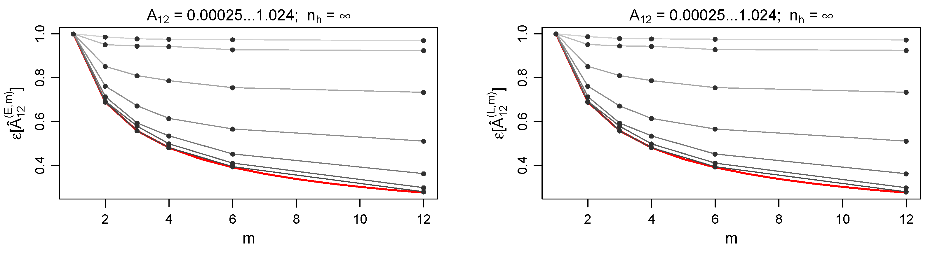
Figure 1 shows the behaviour of $\epsilon \left[{\widehat{A}}_{12}^{\left(m\right)}\right]$ as a function of m, comparing various choices of ${\mathit{\sigma }}_{\Gamma }$. In this case we are not considering yet the contribution to error due to the finite population ($n_h=\infty$ for each cluster h). Equation (54) (red curve) is almost perfectly verified by the least volatility scenario (${\mathit{\sigma }}_{\Gamma }=(2.5,5.0)·{10}^{-2}$). At increasing volatility values (brighter curves), the gain in precision obtained at higher m is reduced, as well as the accordance with Equation (54).

Figure 1. Precision gain ${\epsilon }_{12}^{\left(m\right)}$, as a function of m and $i_{\sigma }$. The left and right plots show the values of $\epsilon \left[{\widehat{A}}_{12}^{(E,m)}\right]$ and $\epsilon \left[{\widehat{A}}_{12}^{(L,m)}\right]$ respectively, as a function of m, for each volatility scenario ($i_{\sigma }=0,\dots ,6$), each depicted with darker to brighter curves, in the $n_h=\infty$ assumption. The red curve is the theoretical value of $\epsilon \left[{\widehat{A}}_{12}^{\left(m\right)}\right]$ in the Gaussian regime.

Since the transformation of $\epsilon \left[{\widehat{A}}_{12}^{\left(m\right)}\right]$ moving away from the Gaussian regime (i.e., increasing $|{\mathit{\sigma }}_{\Gamma }|$) is smooth, estimating $A_{12}$ with $m>1$ remains convenient even for ${\left[{\mathit{\sigma }}_{\Gamma }\right]}_k\gtrsim 1$, despite the fact that Equation (54) is not verified anymore.

Comparison between the left and the right panel of Figure 1 shows that the above argument holds both in the linear and in the exponential case. This fact is also verified for all the other results of this section.

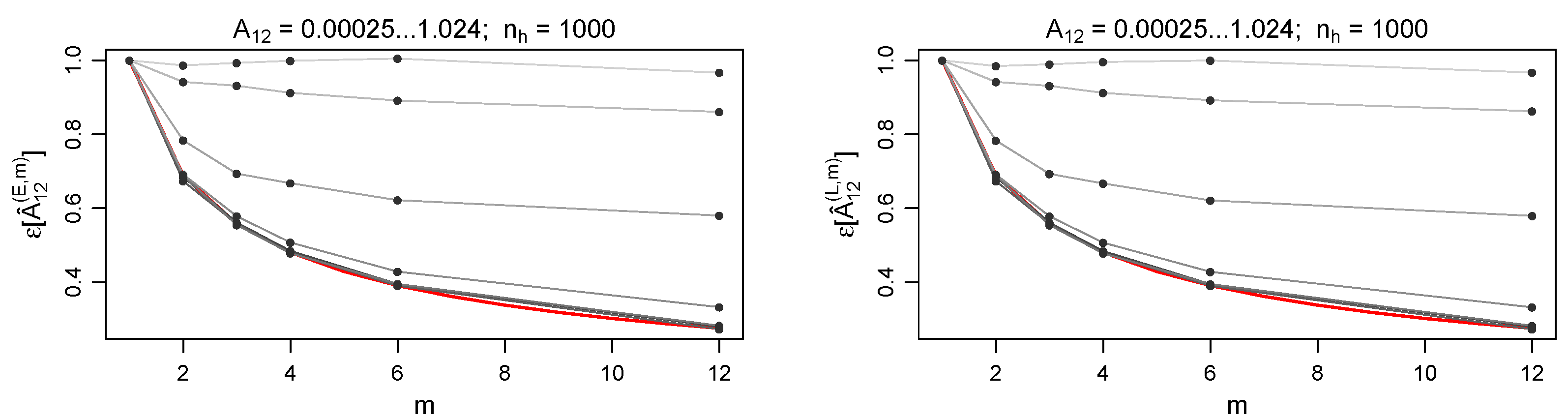
The results shown in Figure 1 are numerically checked against the case of finite portfolio populations: we tested each of the $n_h$ declared in Equation (57). Even the smallest size considered (i.e., $n_h={10}^3$—Figure 2), that is affected by the largest binomial contribution to the error, leads to results comparable to the ones observed in the $n_h=\infty$ case. The size $n_h={10}^3$ is considered to be a limiting value for a realistic case.

Figure 2. $\epsilon \left[{\widehat{A}}_{12}^{(E,m)}\right]$ and $\epsilon \left[{\widehat{A}}_{12}^{(L,m)}\right]$ as a function of m, considering increasing $i_{\sigma }$ (from darker to brighter curve) and $n_h={10}^3$. The red curve is the theoretical value of $\epsilon \left[{\widehat{A}}_{12}^{\left(m\right)}\right]$ as a function of m in the Gaussian regime. For ${\sigma }_1,{\sigma }_2\ll 1$ the analytical result is perfectly satisfied. However, $\epsilon \left[{\widehat{A}}_{12}^{(L,m)}\right]$ is shown to be a decreasing function of m in general. Comparing this result with the $n_h=\infty$ case, we can state that $\epsilon \left[{\widehat{A}}_{h{h}^{\prime }}^{(L,m)}\right]$ is almost insensitive to $n_h$ ($h=1,2$).

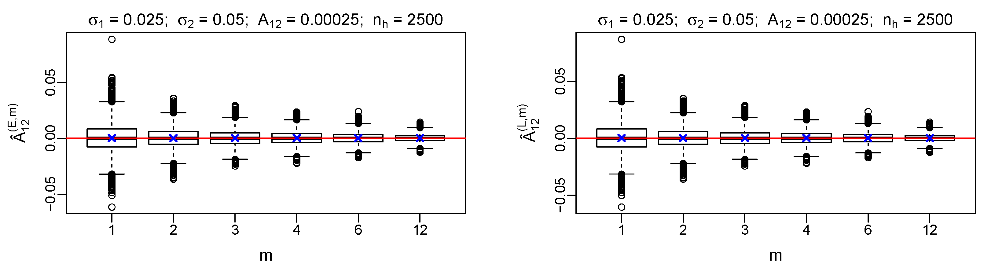
We simulated the distribution of the estimator ${\widehat{A}}_{12}^{\left(m\right)}$ as a function of m, testing all the possible combinations of ${\mathit{\sigma }}_{\Gamma }$ and $n_h$ declared in Equations (55) and (57). Figure 3 reports an example of the results. All the other considered $(n_h,{\sigma }_k)$ couples resulted to have a similar behavior. The visual comparison between $\mathbf{E}\left[{\widehat{A}}_{12}^{\left(m\right)}\right]$ (blue “X” symbol) and $A_{12}$ level (red horizontal line) shows that indeed ${\widehat{A}}_{12}^{\left(m\right)}$ is unbiased, both in the linear and in the exponential case (Equations (37) and (42) respectively). The dispersion around the mean reduces at increasing m, in agreement with both Equation (54) and the numerical results in Figure 1 and Figure 2.

Figure 3. Boxplot of ${\widehat{A}}_{12}^{(E,m)}$ and ${\widehat{A}}_{12}^{(L,m)}$ distributions, as a function of m. The red horizontal line represent the true value of $A_{12}$ and the blue X’s stand for the average value of ${\widehat{A}}_{12}^{\left(m\right)}$.

As implied by Figure 2 and Figure 3, the number of risks $n_h$ does not play a relevant role (if any) in computing the ratio $\epsilon \left[{\widehat{A}}_{12}^{\left(m\right)}\right]$, while the absolute value of the standard error $\sigma \left[{\widehat{A}}_{12}^{\left(m\right)}\right]$ is sensitive to the size of the portfolio.

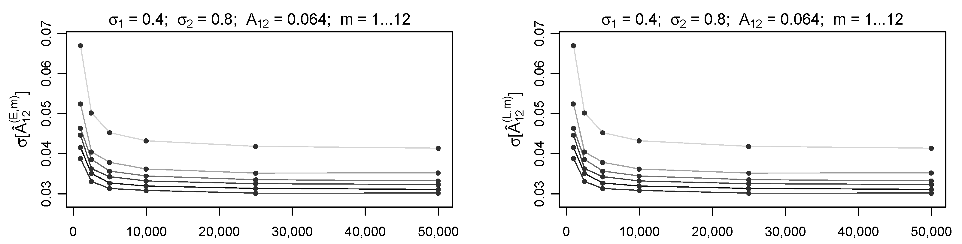
This fact is confirmed by the results shown in Figure 4, where the estimates of $\sigma \left[{\widehat{A}}_{12}^{\left(m\right)}\right]$ have been arranged as functions of $n_h$ at fixed ${\mathit{\sigma }}_{\Gamma }$ and m values. As expected, the standard error is greater when considering smaller $n_h$ values, while the dependence on $n_h$ of the error disappears quickly as approaching $n_h\to \infty$.

Figure 4. $\sigma \left[{\widehat{A}}_{12}^{(E,m)}\right]$ and $\sigma \left[{\widehat{A}}_{12}^{(L,m)}\right]$ as a function of $n_h$. Decreasing m values are considered from darker to brighter curve.

5.3. Estimation Error in Presence of Autocorrelation

In Section 5.2 the precision gain at increasing m is measured in absence of autocorrelation. In this section, the same numerical simulations are re-performed, introducing autocorrelation and comparing the results against the theoretical estimation of $\epsilon$. The effect of autocorrelation on $\epsilon$ is discussed in Appendix B.

The numerical setup introduced above in Section 5.2 has been maintained, with a further assumption about ACF. Indeed, we assume that each latent variable ($k=1,2$) obeys to the following ACF law, discussed in Section 3.3

$${\varrho }_{xk}={\rho }^{\left|x\right|},m=12$$

where the considered $\rho$ values are $0.05$ and $0.5$. For $m^{\prime }<12$ cases, we have considered ACF’s resulting for the latent variables time series ${\tilde{\Gamma }}_k^{\left(j^{\prime }\right)}$ obtained by the clustering operation

$${\tilde{\Gamma }}_k^{\left(j^{\prime }\right)}\equiv \frac{m^{\prime }}{m}\sum _j{\Gamma }_k^{\left(j\right)},j=1+\frac{m}{m^{\prime }}(j^{\prime }-1)\dots \frac{m}{m^{\prime }}{j}^{\prime }$$

given the aforementioned ACF law at $1/m$ time scale. Since the contribution of the finite population to the error has been shown to be neglectable in Section 5.2, simulations in presence of autocorrelation have been performed under $n_h=\infty$ assumption only.

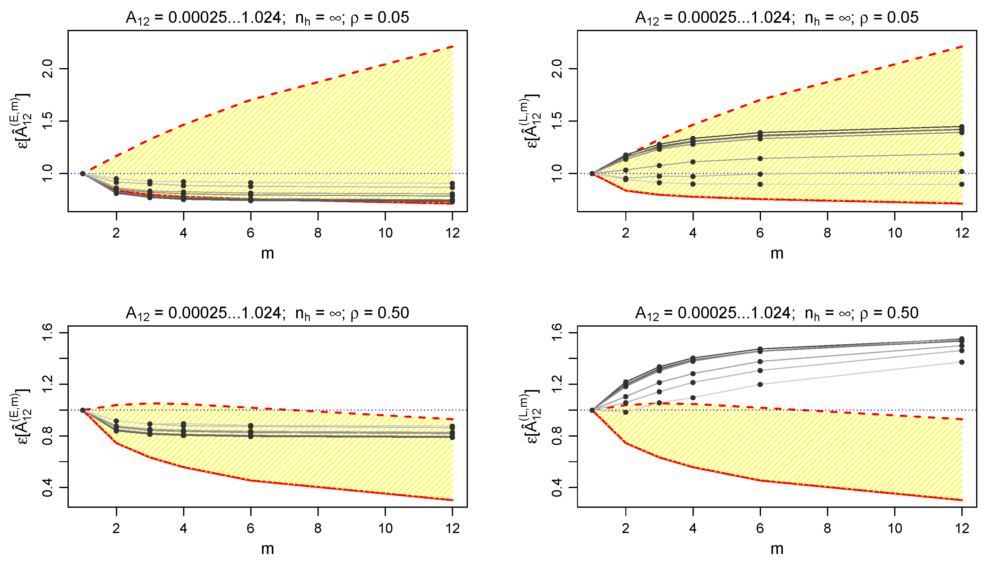
Figure 5 shows that the estimator ${\widehat{A}}_{h{h}^{\prime }}^{(E,m)}$ remains more precise at increasing m, even in presence of autocorrelation. The analytical results obtained in the Gaussian regime (i.e., theoretical superior and inferior estimates of $\epsilon$—dashed and solid red lines in Figure 5), discussed in Appendix B, are in good agreement with the numerical results obtained in the considered set up. All the empirical measures of $\epsilon$ are included between the two theoretical limits (yellow areas).

Figure 5. Precision gain in presence of autocorrelation. $\epsilon \left[{\widehat{A}}_{12}^{(E,m)}\right]$ (exact—left panels) and $\epsilon \left[{\widehat{A}}_{12}^{(L,m)}\right]$ (2nd order approximation—right panels), for each volatility scenario ($i_{\sigma }=0,\dots ,6$, depicted with darker to brighter curves), for $\rho =0.05$ (top) and $\rho =0.5$ (bottom). The yellow area includes all the values between the maximum (dashed red line) and the minimum (solid red line) expected from the results of Appendix B. The frontier $\epsilon =1$ (dotted line) allows to check the presence of a precision gain at $m>1$.

Moreover, precision gain (i.e., $\epsilon <1$) at $m>1$ is also possible when using the estimator $\epsilon \left[{\widehat{A}}_{12}^{(L,m)}\right]$, introduced in Equation (46). However, due to the approximation introduced in this case, the estimator is not convenient (i.e., $\epsilon >1$) in the majority of the considered configurations.

6. An Application to Market Data

This section provides an example of the calibration technique applied to a real-world data set. The calibration technique is applied to a set of historical time series of bad loan rates supplied from the Bank of Italy. “Bad loan” is a subcategory of the broader class “Non-Performing Loan” and it is defined as exposures to debtors that are insolvent or in substantially similar circumstances [24].

In particular, the chosen data set is composed of the quarterly historical series TRI30496 ($m=4$) over a five year period (from 1 January 2013 to 31 December 2017, $n=5$, ${\Delta }_t=1$). The data are publicly available at [10]. The time series are supplied by the customer sector (“counterpart institutional sector”) and geographic area (“registered office of the customer”). The latter, in the example, is held fixed to a unique value that corresponds to the whole country (Italy). Table 2 and Table 3 report the definition of the 6 different clusters and their main features.

Table 2. Definition of the clusters $h=1,\dots ,6$ used in data set TRI30496.

Cluster Index h	Sector Code	Description
1	600	Consumer households
2	S11	Non-financial companies
3	S12BI7	Financial companies other than monetary financial institutions
4	S13	General government
5	S14BI4	Producer households
6	S15BI1	Non-profit institutions serving households and unclassifiable units

Table 3. Main features of the considered historical time series over the period 1 January 2013–31 December 2017. ${\overline{p}}_h$ ($h=1,\dots ,6$) is the yearly average bad loan rate; ${\sigma }_h$ is the volatility associated to each ${\overline{p}}_h$; $⟨n_h⟩$ is the average number of borrowers.

h	1	2	3	4	5	6
${\overline{p}}_h$	0.0119	0.0352	0.0255	0.0056	0.0259	0.0088
${\sigma }_h$	0.0010	0.0042	0.0023	0.0014	0.0022	0.0010
$⟨n_h⟩$	269,515	407,602	3191	5416	132,179	4020

By inspection of Table 3, it is possible to perform a rough estimate of ${\mathit{\sigma }}_{\Gamma }$. Equation (14) implies that the following holds for coefficients of variation $C{V}_h$ ($h=1,\dots ,H\equiv 6$):

$$C{V}_h:=\frac{{\sigma }_h}{{\overline{p}}_h}\simeq \sum _{k=1}^K{\omega }_{hk}{\left[{\mathit{\sigma }}_{\Gamma }\right]}_k$$

Furthermore, the normalization requirement over the factor loadings ${\omega }_{hk}$ implies

$$\sum _{k=1}^K{\omega }_{hk}\lesssim 1$$

Hence we can state that $⟨CV⟩:=\frac{1}{H}{\sum }_{h}C{V}_h$ has the same order of magnitude of $\frac{1}{K}{\sum }_k{\left[{\mathit{\sigma }}_{\Gamma }\right]}_k$. Since $⟨CV⟩\simeq 0.124$, results in Section 5.2 suggest that this data set is not far from the Gaussian regime and so there is an appreciable increase of precision in estimating $A(0,1)$ with $m>1$.

$\widehat{A}(0,1)$ is estimated by applying Equation (42) over a one-year period. The results obtained for ${\widehat{A}}^{(E,m)}(0,1)$ ($m=1,4$) are reported in Table 4.

Table 4. Values of ${\widehat{A}}^{(E,m)}(0,1)$ ($m=4$ left, $m=1$ right) obtained from the quarterly historical series TRI30496 over the period 1 January 2013–31 December 2017. Results are expressed in ${10}^{-2}$ units.

0.53	0.28	0.33	0.36	0.41	0.48	0.68	0.40	0.36	1.01	0.56	0.73
0.28	0.59	0.48	0.61	0.43	0.40	0.40	1.50	0.98	1.26	0.87	−0.16
0.33	0.48	0.67	0.52	0.43	0.40	0.36	0.98	0.87	0.78	0.72	0.27
0.36	0.61	0.52	7.80	0.48	0.33	1.01	1.26	0.78	6.50	1.10	0.66
0.41	0.43	0.43	0.48	0.47	0.54	0.56	0.87	0.72	1.10	0.74	0.47
0.48	0.40	0.40	0.33	0.54	1.53	0.73	−0.16	0.27	0.66	0.47	1.35

The elementwise precision gain for $m=4$, $\epsilon \left[{\widehat{A}}^{(E,4)}(0,1)\right]$, obtained under the Gaussian regime assumption, is shown in Table 5. This result is obtained applying definition (51) and Equation (A25) both to the cases $m=4$ and $m=1$. Equation (A25) has been shown to be valid under the Gaussian regime, discussed in Section 5.1.

Table 5. The elementwise precision gain $\epsilon \left[{\widehat{A}}^{(E,4)}(0,1)\right]$ associated with results reported in Table 4.

0.36	0.26	0.37	0.41	0.33	0.39
0.26	0.18	0.24	0.30	0.23	0.33
0.37	0.24	0.35	0.43	0.30	0.45
0.41	0.30	0.43	0.55	0.37	0.52
0.33	0.23	0.30	0.37	0.29	0.42
0.39	0.33	0.45	0.52	0.42	0.52

In this case, the preliminary decomposition of ${\widehat{A}}^{(E,4)}(0,1)$, that would be needed using the Monte Carlo method discussed in Section 5.2, is not needed.

According to Equation (54), the elements of $\epsilon \left[{\widehat{A}}^{(E,4)}(0,1)\right]$ reported in Table 5 should be all approximately equal to $0.46$, since they should depend only on the couple $m,n$ ($m=4$ and $n=5$ in this case). However, in a real world case like the one considered, the assumption of zero autocorrelation is satisfied with a different precision by each time series $p_h\left(t\right)$. Furthermore, the estimated covariance matrices might need to be regularized (indeed the Higham regularization algorithm [25] was used both for $m=1$ and $m=4$ series). Hence, a different ratio for each element $(h,h^{\prime })=1,\dots ,6$ is justified. Nonetheless, it is worth noticing that all the ratios reported in Table 5 have the same order of magnitude of the predicted value $0.46$.

Knowledge of the historical number of risky subjects $n_h\left(t\right)$ for each cluster ($h=1,\dots ,6$) at each observation date ($t=1/4,2/4,\dots ,5$) allows to take into account the binomial contribution to the error $\sigma \left[{\widehat{A}}^{(E,m)}(0,1)\right]$, both for $m=4$ (quarterly series) and $m=1$ (yearly series), although the finiteness of the population does not add a relevant contribution to the error, as already observed in Section 5.2.

Table 6 provides Monte Carlo estimation of $\sigma \left[{\widehat{A}}^{(E,m)}(0,1)\right]$$(m=1,4)$, which considers also the role of $n_h\left(t\right)$. Since the values in Table 6 provide a measure of the error in the determination of ${\widehat{A}}^{(E,m)}(0,1)$, it turns out that the estimates reported in Table 4 are elementwise consistent one with the other.

Table 6. $\sigma \left[{\widehat{A}}^{(E,m)}(0,1)\right]$ ($m=4$ left, $m=1$ right). These are the elementwise errors of the estimators reported in Table 4. The results above are expressed in ${10}^{-2}$ units.

0.11	0.12	0.19	0.44	0.11	0.31	0.41	0.25	0.41	1.09	0.24	0.64
0.12	0.20	0.29	0.64	0.13	0.40	0.25	0.86	0.72	1.47	0.50	0.97
0.19	0.29	1.38	1.08	0.21	0.69	0.41	0.72	1.75	2.31	0.49	1.53
0.44	0.64	1.08	5.12	0.49	1.60	1.09	1.47	2.31	9.11	1.20	3.40
0.11	0.13	0.21	0.49	0.13	0.34	0.24	0.50	0.49	1.20	0.29	0.79
0.31	0.40	0.69	1.60	0.34	3.25	0.64	0.97	1.53	3.40	0.79	4.65

The Monte Carlo estimation of $\sigma \left[{\widehat{A}}^{(E,m)}(0,1)\right]$, as done in Section 5.2, requires the a priori knowledge of the true dependence structure $W,{\mathit{\sigma }}_{\Gamma }$. Since this is a case study, we do not have an a priori parameterization of the calibrated model. Hence, we have used $\widehat{W},{\widehat{\mathit{\sigma }}}_{\Gamma }$ estimated from ${\widehat{A}}^{(E,4)}(0,1)$ instead, as a proxy of the “true” model parameters. The computation of $\widehat{W},{\widehat{\mathit{\sigma }}}_{\Gamma }$ from ${\widehat{A}}^{(E,4)}(0,1)$ is discussed below.

In order to complete the CreditRisk${}^{+}$ calibration, we have to decompose $\widehat{A}$ and find the factor loadings matrix $\widehat{W}$ together with the vector of systematic factors variances ${\widehat{\mathit{\sigma }}}_{\Gamma }^2$. To do so, we use the Symmetric Non-negative Matrix Factorization (SNMF), an iterative numerical method to search an approximate decomposition of $\widehat{A}$ which satisfies the requirements of the CreditRisk${}^{+}$ model over $\widehat{W}$ (i.e., all elements ${\omega }_{hk}>0$ and ${\sum }_k{\omega }_{hk}=1$). The application of SNMF to CreditRisk${}^{+}$ is discussed in detail in [14]. In the following, we give evidence only of the implementation details necessary to address this case study. Being an iterative method, SNMF requires an initial choice of matrixes

$$\begin{array}{ccc}\hfill {\widehat{U}}_0& :=& {\widehat{W}}_U{\widehat{\Sigma }}^{1/2},\hfill \\ \hfill {\widehat{V}}_0& :=& {\widehat{\Sigma }}^{1/2}{\widehat{W}}_V,\hfill \end{array}$$

such that $\widehat{A}={\widehat{U}}_0{\widehat{V}}_0$. It is not required that ${\widehat{U}}_0={\widehat{V}}_0^T$, nor all the elements of ${\widehat{U}}_0$ and ${\widehat{V}}_0$ have to be positive. We set ${\widehat{U}}_0,{\widehat{V}}_0$ from the eigenvalues decomposition of ${\widehat{A}}^{(E,4)}(0,1)$.

For the considered data set, the eigenvalues decomposition returned the set of eigenvalues and eigenvectors reported in Table 7.

Table 7. Set of eigenvalues ${\tilde{\sigma }}_k$ and eigenvectors ${\tilde{\mathit{\omega }}}_k$ obtained by the eigenvalues decomposition of ${\widehat{A}}^{(E,4)}(0,1)$, as reported in Table 4.

${\tilde{\mathit{\omega }}}_{\mathit{k}}$	k = 1	k = 2	k = 3	k = 4	k = 5	k = 6
	0.06	−0.34	0.13	0.84	0.00	0.39
	0.10	−0.33	0.43	−0.38	−0.65	0.36
	0.09	−0.36	0.52	−0.26	0.72	0.06
	0.98	0.17	−0.07	0.01	0.01	0.00
	0.08	−0.38	0.22	0.19	−0.22	−0.84
	0.07	−0.68	−0.69	−0.20	0.06	0.07
${\tilde{\sigma }}_k^2$	0.08	0.02	0.01	2.9 · ${10}^{-3}$	1.4 · ${10}^{-3}$	0.3 · ${10}^{-3}$

We use the $\tilde{\mathit{\omega }},\tilde{\sigma }$ notation to address the quantities over which the normalization requirement of CreditRisk${}^{+}$ has not been imposed yet.

Since more than the $95\%$ of variance is explained by the first three eigenvectors, we reduced the dimensionality of the latent variables vector to be $K=3$. Hence we define

$$\begin{array}{ccc}\hfill {\widehat{U}}_0& =& \left[{\tilde{\mathit{\omega }}}_1,{\tilde{\mathit{\omega }}}_2,{\tilde{\mathit{\omega }}}_3\right]\hspace{0.17em}·\hspace{0.17em}\mathrm{diag}({\tilde{\sigma }}_1,{\tilde{\sigma }}_2,{\tilde{\sigma }}_3)\hfill \\ & =& \left[\begin{array}{ccc}\hfill 1.80& \hfill 5.29& \hfill 1.15\\ \hfill 2.78& \hfill 5.18& \hfill 3.71\\ \hfill 2.51& \hfill 5.58& \hfill 4.46\\ \hfill 27.79& \hfill -2.65& \hfill -0.57\\ \hfill 2.33& \hfill 5.88& \hfill 1.93\\ \hfill 2.07& \hfill 10.58& \hfill -5.96\end{array}\right]\hspace{0.17em}·\hspace{0.17em}{10}^{-2}\hfill \end{array}$$

and ${\widehat{V}}_0={\widehat{U}}_0^T$. In general, SNMF aims to minimize iteratively the cost function

$${\left|\widehat{A}-\widehat{U}\widehat{V}\right|}^2+\alpha {\left|\widehat{U}-{\widehat{V}}^T\right|}^2$$

where $|·|$ is the Frobenious norm, eventually weighted, and $\alpha$ is a free parameter to weight the asymmetry penality term. Further details on the method are available in [14]. The application of SNMF method, together with the normalization constraint over the factor loadings, leads to the result reported in Table 8.

Table 8. The complete set of parameters $\widehat{W},{\widehat{\mathit{\sigma }}}_{\Gamma }^2$ necessary to specify the dependence structure in CreditRisk${}^{+}$ model, obtained by the eigenvalues decomposition of ${\widehat{A}}^{(E,4)}(0,1)$, as reported in Table 4.

k	0	1	2	3
${\omega }_{1k}$	0.67	0.04	0.29	0.00
${\omega }_{2k}$	0.07	0.07	0.27	0.59
${\omega }_{3k}$	0.00	0.06	0.28	0.66
${\omega }_{4k}$	0.13	0.87	0.00	0.00
${\omega }_{5k}$	0.63	0.06	0.31	0.00
${\omega }_{6k}$	0.29	0.04	0.67	0.00
${\sigma }_k^2$		0.103	0.031	0.010

A reasonable economic interpretation supports the set of parameters resulting from the calibration process described above. Indeed, factor loadings associated with the “general government” sector ($h=4$) are completely distinct from the ones of the other sectors (i.e., this is the only sector mainly depending on the $k=1$ factor): this fact copes with the different nature of the public entities from the ones belonging to the other considered sectors. Furthermore, “companies” ($h=2,3$) share approximately the same dependence structure. The same applies when considering “households” ($h=1,5$). Finally, the “institutions serving households” sector ($h=6$) shares the same latent factor ($k=2$) but shows a different balance between idiosyncratic and systematic factor loadings compared to “households”, that is coherent with the nature of a sector strongly linked to “household” sectors, despite not being completely equivalent.

Results in Table 8 have been used to quantify the estimation errors reported in Table 6.

7. Conclusions

In this work, we have investigated how to calibrate the dependence structure of the CreditRisk${}^{+}$ model, when the sampling period ${\delta }_m$ of the (available) default rate time series is different from ${\Delta }_t$—the length of the future time interval chosen for the projections.

Preliminarily, we proved that CreditRisk${}^{+}$ remains internally consistent when imposing the underlying distributional assumption to be simultaneously true at different time scales (Theorem 1). The model internal consistency is robust against the introduction of autocorrelation, depending on the considered ACF form (Theorem 2).

Then the problem has been approached in terms of moment matching, providing two asymptotically equivalent formulations for estimating the covariance matrix A amongst the systematic factors of the model (Propositions 2 and 3). The choice between the two estimators of A, provided in Equations (37) and (42), depends on the functional form (linear or exponential) that links the probability of claim/default and the latent variables. Both the estimators are explicitly dependent on the ratio ${\Delta }_t/{\delta }_m$, allowing for the calibration of the model at a time scale that is different from the one chosen for applying the calibrated model. Both the estimators have been generalized to autocorrelated time series in Equations (46) and (49), although only the latter (i.e., exponential case) is an exact result, while a second-order approximation has been adopted for the linear case.

Furthermore, calibrating the model on a shorter time scale than the projection horizon has been proved to be convenient in terms of reduced estimation error on $\widehat{A}$. Analytical expressions for the error are provided in the Gaussian regime (i.e., small variances of the latent variables) by Theorem 3. In contrast, the case of increasing variance has been investigated numerically, confirming that, in general, the precision of the calibration is higher when employing historical data with a shorter sampling period. It has been verified that the convenience of calibrating the model at short time scales also remains in the presence of autocorrelation, although this is guaranteed only in the exponential framework, where an exact correction term is available.

Finally, the techniques presented in this work are shown to be numerically sound when applied to a real, publicly available data set of Italian bad loan rates.

Appendix A.1. Proof of Theorem 1

Proof. 

Firstly, the statement is proved considering Assumptions 1 and 3.

Assumption 3 implies by construction that ${\left\{Y_i^{\left(j\right)}\right\}}_{j=1\dots m}$ is a set of Poisson r.v.’s, which are mutually independent, conditionally on the realization of ${\left\{{\mathbf{\Gamma }}^{\left(j\right)}\right\}}_{j=1\dots m}$. Poisson distribution is closed with respect to addition. Hence

$$\sum _{j=1}^m{Y}_i^{\left(j\right)}|{\mathbf{\Gamma }}^{\left(j\right)}\sim \mathrm{Poisson}\left(p_{i\Sigma }\right),$$

(A1)

where the distribution parameter is

$$p_{i\Sigma }=\sum _{j=1}^m\underset{q_i^{\left(j\right)}}{\underbrace{q_i\frac{t_j-t_{j-1}}{T-t}}}\left({\displaystyle {\omega }_{i0}+\sum _{k=1}^K{\omega }_{ik}{\Gamma }_k^{\left(j\right)}}\right).$$

(A2)

Equation (20) in Assumption 3, the choice ${\xi }_{kj}=1$ and the scaling property of Gamma distribution imply that

$$\frac{t_j-t_{j-1}}{T-t}{\Gamma }_k^{\left(j\right)}\sim \mathrm{Gamma}\left({\sigma }_k^{-2}\frac{t_j-t_{j-1}}{T-t},{\sigma }_k^2\right)$$

(A3)

Furthermore, Assumption 5 and the fact that independent Gamma r.v.’s with the same scale parameter are closed with respect to addition imply that

$$\sum _{j=1}^m\frac{t_j-t_{j-1}}{T-t}{\Gamma }_k^{\left(j\right)}\sim \mathrm{Gamma}\left({\sigma }_k^{-2},{\sigma }_k^2\right).$$

(A4)

Hence ${\sum }_{j=1}^m\frac{t_j-t_{j-1}}{T-t}{\Gamma }_k^{\left(j\right)}\equiv {\Gamma }_k$ and so ${\sum }_{j=1}^m{Y}_i^{\left(j\right)}\equiv Y_i$. This implies that $\left\{Y_i\right\}$ satisfies Assumption 1 over $(t,T]$.

The proof above can be extended to the exponential case, i.e., when considering Assumptions 2 and 4 instead of Assumptions 1 and 3. The form of parameter $p_{i\Sigma }$ in (A2) can be obtained also can be obtained also from Assumption 4. In fact, the substitution $Y_i^{\left(j\right)}\mapsto {\tilde{Y}}_i^{\left(j\right)}$ implies that ${\tilde{Y}}_i\sim \mathrm{Bernoulli}\left({\tilde{p}}_i\right)$ where

$$ln\left(1-{\tilde{p}}_i\right)\hspace{0.17em}=\hspace{0.17em}ln\prod _{j=1}^m\left(1-{\tilde{p}}_i^{\left(j\right)}\right)\hspace{0.17em}=\hspace{0.17em}\sum _{j=1}^m{q}_i\frac{t_j-t_{j-1}}{T-t}\left({\displaystyle {\omega }_{i0}+\sum _{k=1}^K{\omega }_{ik}{\Gamma }_k^{\left(j\right)}}\right).$$

(A5)

Considering Equation (A5) instead of (A2), the proof presented above holds for the ${\tilde{Y}}_i$ representation of risks, ceteris paribus, implying that $\left\{{\tilde{Y}}_i\right\}$ satisfies Assumption 2 over $(t,T]$. □

Appendix A.2. Proof of Theorem 2

Proof. 

The same arguments that lead to (A2) or to (A5) in proof of Theorem 1 are still valid in this case. Hence, it suffices to prove that mean and variance of the latent variable

$${\Gamma }_k^{\prime }:=\sum _{j=1}^m\frac{t_j-t_{j-1}}{T-t}{\Gamma }_k^{\left(j\right)}=\frac{1}{m}\sum _{j=1}^m{\Gamma }_k^{\left(j\right)}$$

remain consistent with CreditRisk${}^{+}$ requirements, stated in Assumption 1. It holds $\mathbf{E}\left[{\Gamma }_k^{\prime }\right]=1$, since $\mathbf{E}\left[{\Gamma }_k^{\left(j\right)}\right]=1$. Moreover, the coefficient ${\xi }_{jk}$ compensates the bias introduced in $\mathbf{var}\left[{\Gamma }_k^{\prime }\right]$ by the fact that ${\Gamma }_k^{\left(j\right)}$ ($j=1\dots m$) are autocorrelated according to the ACF ${\varrho }_{xk}$:

$$\begin{array}{ccc}\hfill \mathbf{var}\left[\sum _{j=1}^m{\Gamma }_k^{\left(j\right)}\right]& =& \sum _{j=1}^m\mathbf{var}\left[{\Gamma }_k^{\left(j\right)}\right]+\sum _{j=1}^m\sum _{j^{\prime }\ne j}\mathbf{cov}\left[{\Gamma }_k^{\left(j\right)},{\Gamma }_k^{\left(j^{\prime }\right)}\right]\hfill \\ & =& \mathbf{var}\left[{\Gamma }_k^{\left(1\right)}\right]\underset{m{\xi }_{kj}^{-2}}{\underbrace{\left(m+2\sum _{x=1}^{m-1}\left(m-x\right){\varrho }_{xk}\right)}}\hfill \end{array}$$

which implies $\mathbf{var}\left[{\Gamma }_k^{\prime }\right]={\sigma }_k^2$ directly.

The fact that ${\Gamma }_k^{\prime }$ is Gamma distributed is imposed in Assumption 6, implying that ${\Gamma }_k^{\prime }\equiv {\Gamma }_k$ and so that Assumption 1 is satisfied. □

Appendix A.3. Proof of Proposition 2

Proof. 

Given a time interval $(t,T]\subseteq (t_a,t_b]$ and a uniform partition ($j=1\dots m$) over $(t,T]$, Assumptions A3 and A5 imply that $\left\{Y_i\right\}$ satisfies Assumption 1 over $(t,T]$ by Theorem 1. Assumption 7 guarantees the convergence of $F_h$ to $\mathbf{E}\left[F_h\right|\mathbf{\Gamma }]$ and of $F_h^{\left(j\right)}$ to $\mathbf{E}\left[F_h^{\left(j\right)}\right|{\mathbf{\Gamma }}^{\left(\mathbf{j}\right)}]$, where we recall that $F_h=F_h(t,T)$.

For any interval $(t,T]\subseteq (t_a,t_b]$ and any pair of clusters $c_h,c_{h^{\prime }}$, definitions (34), (35) and Assumption 5 imply that the covariance between $F_{mh}$ and $F_{m{h}^{\prime }}$ is given by

$$\mathbf{cov}\left(F_{mh},F_{m{h}^{\prime }}\right)\hspace{0.17em}=\hspace{0.17em}\prod _{j=1}^m\left[\mathbf{cov}\left(F_h^{\left(j\right)}{F}_{h^{\prime }}^{\left(j\right)}\right)\hspace{0.17em}+\hspace{0.17em}{s}_h^{\left(j\right)}{s}_{h^{\prime }}^{\left(j\right)}\right]-s_h{s}_{h^{\prime }}$$

(A6)

Since all the considered subintervals $(t_{j-1},t_j]$ have the same length ${\delta }_m=t_j-t_{j-1}$, the frequencies $F_h^{\left(j\right)}$ are i.i.d., so that the above expression simplifies to:

$$\mathbf{cov}\left(F_{mh},F_{m{h}^{\prime }}\right)\hspace{0.17em}+\hspace{0.17em}{s}_h{s}_{h^{\prime }}={\left[\mathbf{cov}\left(F_h^{\left(j\right)},F_{h^{\prime }}^{\left(j\right)}\right)\hspace{0.17em}+\hspace{0.17em}{s}_h^{\left(j\right)}{s}_{h^{\prime }}^{\left(j\right)}\right]}^m$$

(A7)

for any $j=1,\dots ,m$.

Each cluster $c_h$ is supposed to be homogenous by definition, i.e., ${\mathit{\omega }}^{\left(i\right)}={\mathit{\omega }}^{\left(h\right)}$ for each risk $Y_i\in c_h$. Hence, distributional Assumptions 1 and 3 imply that both $F_h\stackrel{n_h\left(t\right)\to \infty }{\to }\mathbf{E}\left[F_h\right|\mathbf{\Gamma }]$ and $F_h^{\left(j\right)}\stackrel{n_h\left(t_j\right)\to \infty }{\to }\mathbf{E}\left[F_h^{\left(j\right)}\right|{\mathbf{\Gamma }}^{\left(\mathbf{j}\right)}]$ are sample estimators of the parameters $p_h(\mathbf{\Gamma }):=q_h({\omega }_{h0}+{\sum }_k{\omega }_{hk}{\Gamma }_k)$ and $p_h^{\left(j\right)}\left({\mathbf{\Gamma }}^{\left(j\right)}\right)$ respectively, leading to the equivalence relation

$$F_{mh}=F_h={\widehat{q}}_h\left({\omega }_{h0}+\sum _{k=1}^K{\omega }_{hk}{\Gamma }_k\right),$$

(A8)

therefore both $F_{mh}(t,T)$ and $F_h(t,T)$ are estimators of the default frequency for the $(t,T]$ interval. Thus, Equation (A7) can be rewritten as:

$$\mathbf{cov}\left(F_h,F_{h^{\prime }}\right)\hspace{0.17em}+\hspace{0.17em}{s}_h{s}_{h^{\prime }}={\left[\mathbf{cov}\left(F_h^{\left(j\right)},F_{h^{\prime }}^{\left(j\right)}\right)\hspace{0.17em}+\hspace{0.17em}{s}_h^{\left(j\right)}{s}_{h^{\prime }}^{\left(j\right)}\right]}^m$$

(A9)

and, since $m=(T-t)/{\delta }_m$,

$${\left[\mathbf{cov}\left(F_h,F_{h^{\prime }}\right)\hspace{0.17em}+\hspace{0.17em}{s}_h{s}_{h^{\prime }}\right]}^{1/(T-t)}={\left[\mathbf{cov}\left(F_h^{\left(j\right)},F_{h^{\prime }}^{\left(j\right)}\right)\hspace{0.17em}+\hspace{0.17em}{s}_h^{\left(j\right)}{s}_{h^{\prime }}^{\left(j\right)}\right]}^{1/{\delta }_m}.$$

(A10)

To complete the proof, let $(t,T]$ and $(t^{\prime },T^{\prime }]$ be two subintervals of $(t_a,t_b]$, such that $(T-t)/(T^{\prime }-t^{\prime })\in \mathbb{Q}$. Hence, $\mathrm{GCD}\{T-t;T^{\prime }-t^{\prime }\}:=\overline{\delta }\in {\mathbb{R}}_{+}$ exists. $\overline{\delta }$ can be used as the mesh to define two uniform partitions over the two considered intervals.

Given these partitions, (A10) can be applied both to $T-t$ and to $T^{\prime }-t^{\prime }$, leading to

$$\begin{array}{ccc}& & {\left[\mathbf{cov}\left(F_h(t,T),F_{h^{\prime }}(t,T)\right)\hspace{0.17em}+\hspace{0.17em}{s}_h(t,T)s_{h^{\prime }}(t,T)\right]}^{1/(T-t)}=\hfill \\ & & {\left[\mathbf{cov}\left(F_h(t^{\prime },T^{\prime }),F_{h^{\prime }}(t^{\prime },T^{\prime })\right)\hspace{0.17em}+\hspace{0.17em}{s}_h(t^{\prime },T^{\prime })s_{h^{\prime }}(t^{\prime },T^{\prime })\right]}^{1/(T^{\prime }-t^{\prime })}\hfill \end{array}$$

and completing the proof. The requirement $(T-t)/(T^{\prime }-t^{\prime })\in \mathbb{Q}$ can be easily weakened by the convergence of finite continued fractions with an increasing number of terms, until the desired degree of precision is reached. □

Appendix A.4. Proof of Proposition 3

Proof. 

Given a time interval $(t,T]\subseteq (t_a,t_b]$ and a uniform partition ($j=1\dots m$) over $(t,T]$, Assumptions 4 and 5 imply that $\left\{{\tilde{Y}}_i\right\}$ satisfies Assumption 2 over $(t,T]$ by Theorem 1.

Assumption 7 guarantees the convergence of $L_h$ to $\mathbf{E}\left[L_h\right|\mathbf{\Gamma }]$, where we recall that $L_h=L_h(t,T)$. Furthermore, it holds by definition that $\mathbf{E}\left[L_h\right|\mathbf{\Gamma }]=p_h(\mathbf{\Gamma })$, where the notation $p_h$ has been introduced in the proof of Proposition 2.

The same apply to $L_h^{\left(j\right)}$ ($j=1\dots m$) for each uniform partition of $(t,T]$ considered; indeed, Assumption 7 implies $L_h^{\left(j\right)}\to \mathbf{E}\left[L_h^{\left(j\right)}\right|{\mathbf{\Gamma }}^{\left(j\right)}]=p_h^{\left(j\right)}(\mathbf{\Gamma })$.

Since $p_h(\mathbf{\Gamma })={\sum }_{j=1}^m{p}_h^{\left(j\right)}\left({\mathbf{\Gamma }}^{\left(j\right)}\right)$ and given that the partition is uniform, it holds $L_h=m{L}_h^{\left(j\right)}$ for each $j=1\dots m$. Since $m(T-t)/{\delta }_m$, we have

$$\frac{1}{T-t}{L}_h=\frac{1}{{\delta }_m}{L}_h^{\left(j\right)}$$

(A11)

Assumption 5 and Equation (A11) imply that

$$\frac{1}{T-t}\mathbf{cov}[L_h,L_{h^{\prime }}]=\frac{1}{{\delta }_m}\mathbf{cov}[L_h^{\left(j\right)},L_{h^{\prime }}^{\left(j\right)}]$$

(A12)

for each considered pair of clusters $c_h,c_{h^{\prime }}$. The proof is completed by the same argument used in proof of Proposition 2, after Equation (A10). □

Appendix A.5. Proof of Theorem 3

Proof. 

Assumptions 3 and 5 and ${\xi }_{kj}=1$ imply Assumption 1 by Theorem 1. The same theorem implies Assumption 2 in case Assumption 4 is considered instead of Assumption 3, ceteris paribus. Furthermore, Assumptions 3, 5 and 7 and ${\xi }_{kj}=1$ imply that

$${\widehat{A}}_{h{h}^{\prime }}^{(L,m)}=\frac{1}{q_h{q}_{h^{\prime }}}\left[{\left({\widehat{c}}_{h{h}^{\prime }}^{\left(Lm\right)}\right)}^m-s_h{s}_{h^{\prime }}-{\delta }_{h{h}^{\prime }}\frac{q_h}{n_h}\right]$$

(A13)

by Proposition 2, for any $j=1\dots m$ and $h,h^{\prime }=1\dots H$. Analogously, considering Assumption 4 instead of Assumption 3, it holds

$${\widehat{A}}_{h{h}^{\prime }}^{(E,m)}=\frac{m}{q_h{q}_{h^{\prime }}}{\widehat{c}}_{h{h}^{\prime }}^{\left(Em\right)}$$

(A14)

by Proposition 3, for any $j=1\dots m$ and $h,h^{\prime }=1\dots H$.

The next step of the proof is showing that ${\Gamma }_k\dot{\sim }\mathcal{N}(1,{\beta }_k)$ in the limit ${\sigma }_k\to 0^{+}$. In fact, both Assumptions 3 and 4 state that

$${\Gamma }_k^{\left(j\right)}\sim \Gamma \left(\frac{1}{m{\beta }_k},m{\beta }_k\right),\mathbf{E}\left[{\Gamma }_k^{\left(j\right)}\right]\hspace{0.17em}=\hspace{0.17em}1,\mathbf{var}\left[{\Gamma }_k^{\left(j\right)}\right]\hspace{0.17em}=\hspace{0.17em}m{\beta }_k,j=1,\dots ,m.$$

Hence their probability densities $d{F}_k\left(x\right)$ satisfy the following:

$$d{F}_k\left(x\right)\propto x^{{\left(m{\beta }_k\right)}^{-1}-1}exp\left(-{\left(m{\beta }_k\right)}^{-1}x\right)dx$$

(A15)

Since it holds ${\left(m{\beta }_k\right)}^{-1}-1\stackrel{{\sigma }_k\to 0^{+}}{\to }{\left(m{\beta }_k\right)}^{-1}$, we have

$${\displaystyle \underset{{\sigma }_k\to 0^{+}}{lim}d{F}_k\left(x\right)\propto exp\left(\frac{lnx-x}{m{\beta }_k}\right)dx.}$$

(A16)

By introducing the auxiliary variable $x^{\prime }x-1$ and replacing $ln(1+x^{\prime })$ with the first three terms of its Maclaurin series, relation (A16) can be equivalently written as

$${\displaystyle \underset{{\sigma }_k\to 0^{+}}{lim}d{F}_k\left(x\left(x^{\prime }\right)\right)\propto exp\left(-\frac{{x^{\prime }}^2}{2m{\beta }_k}\right)d{x}^{\prime }}$$

(A17)

In the limit ${\sigma }_k={\beta }_k\to 0^{+}$, Equation (A17) implies that

$${\Gamma }_k^{\left(j\right)}\sim \mathcal{N}\left(\mu =1,{\sigma }^2=m{\beta }_k\right).$$

(A18)

Hence it holds that each $F_h^{\left(j\right)}$ is normally distributed, with variance $m{\sigma }_h^2:=m{\sum }_k{\omega }_{hk}{\beta }_k$—when considering the linear case (i.e., Assumptions 1 and 3). Analogously, also each $L_h^{\left(j\right)}$ is normally distributed in the exponential case (i.e., Assumptions 2 and 4).

Considering the market factors—as well as the historical observations of default frequency—as normal random variables is relevant to prove the theorem, since it implies that the covariance matrix estimators ${\widehat{c}}^{\left(Lm\right)}$ and ${\widehat{c}}^{\left(Em\right)}$ are Wishart distributed. Hence the variance associated to a given matrix element is

$$\mathbf{var}\left[{\widehat{c}}_{h{h}^{\prime }}^{\left(m\right)}\right]\hspace{0.17em}=\hspace{0.17em}\frac{m^2}{m·n-1}\left({\rho }_{h{h}^{\prime }}^2+1\right){\sigma }_h^2{\sigma }_{h^{\prime }}^2$$

(A19)

in both linear and exponential cases. In the exponential case Equation (A19) is equivalent to the following

$$\mathbf{var}\left[{\widehat{c}}_{h{h}^{\prime }}^{\left(Em\right)}\right]\hspace{0.17em}=\hspace{0.17em}\frac{1}{m·n-1}\left[{\left(c_{h{h}^{\prime }}^{\left(Em\right)}\right)}^2+c_{hh}^{\left(Em\right)}{c}_{h^{\prime }{h}^{\prime }}^{\left(Em\right)}\right]$$

(A20)

while the same is not true in the linear case. Given Equation (A19), it is possible to prove Equation (54) separately in the two cases.

Proof in the linear case. Proposition 2 implies

$$\begin{array}{ccc}\hfill \mathbf{var}\left[{\widehat{A}}_{h{h}^{\prime }}^{(L,m)}\right]& =& \frac{1}{{\left(q_h{q}_{h^{\prime }}\right)}^2}\mathbf{var}\left[{\left({\widehat{c}}_{h{h}^{\prime }}^{\left(Lm\right)}\right)}^m\right]\hspace{0.17em}=\hspace{0.17em}\frac{1}{{\left(q_h{q}_{h^{\prime }}\right)}^2}\left[{\left(\mathbf{E}\left[{\left(\left.{\left.{\widehat{c}}_{h{h}^{\prime }}^{\left(Lm\right)}\right)}^2\right]\right)}^m-\right(\mathbf{E}\left[{\widehat{c}}_{h{h}^{\prime }}^{\left(Lm\right)}\right]\right)}^{2m}\right]\hfill \\ & =& \frac{1}{{\left(q_h{q}_{h^{\prime }}\right)}^2}\left[{\left(\mathbf{var}\left[{\widehat{c}}_{h{h}^{\prime }}^{\left(Lm\right)}\right]\hspace{0.17em}+\hspace{0.17em}{\left(\mathbf{E}\left[{\widehat{c}}_{h{h}^{\prime }}^{\left(Lm\right)}\right]\right)}^2\right)}^m-{\left(\mathbf{E}\left[{\widehat{c}}_{h{h}^{\prime }}^{\left(Lm\right)}\right]\right)}^{2m}\right]\hfill \end{array}$$

(A21)

In the limit $\mathit{\sigma }\to {\mathbf{0}}^{+}$ the binomial above can be replaced with its leading term. Hence

$$\mathbf{var}\left[{\widehat{A}}_{h{h}^{\prime }}^{(L,m)}\right]\hspace{0.17em}=\hspace{0.17em}\frac{1}{{\left(q_h{q}_{h^{\prime }}\right)}^2}\mathbf{var}\left[{\widehat{c}}_{h{h}^{\prime }}^{\left(Lm\right)}\right]{\left(\mathbf{E}\left[{\widehat{c}}_{h{h}^{\prime }}^{\left(Lm\right)}\right]\right)}^{2(m-1)}$$

(A22)

By applying Equation (A19) we have

$$\begin{array}{ccc}\hfill \mathbf{var}\left[{\widehat{A}}_{h{h}^{\prime }}^{(L,m)}\right]& =& \frac{1}{{\left(q_h{q}_{h^{\prime }}\right)}^2}\frac{m^2}{m·n-1}\left({\rho }_{h{h}^{\prime }}^2+1\right){\sigma }_h^2{\sigma }_{h^{\prime }}^2{\left(c_{h{h}^{\prime }}^{\left(Lm\right)}\right)}^{2(m-1)}\hfill \\ & =& \frac{1}{{\left(q_h{q}_{h^{\prime }}\right)}^2}\frac{1}{m·n-1}\frac{{\rho }_{h{h}^{\prime }}^2+1}{{\rho }_{h{h}^{\prime }}^2}{\left(c_{h{h}^{\prime }}^{\left(Lm\right)}-s_h^{\left(j\right)}{s}_{h^{\prime }}^{\left(j\right)}\right)}^2{\left(c_{h{h}^{\prime }}^{\left(Lm\right)}\right)}^{2(m-1)}\hfill \end{array}$$

(A23)

Applying Proposition 2 once again we have ${\left(c_{h{h}^{\prime }}^{\left(Lm\right)}\right)}^{2m}={\left(c_{h{h}^{\prime }}^{\left(L1\right)}\right)}^2$. Furthermore, we have $s_h^{\left(j\right)}{s}_{h^{\prime }}^{\left(j\right)}{\left(c_{h{h}^{\prime }}^{\left(Lm\right)}\right)}^{2(m-1)}\stackrel{\mathit{\sigma }\to {\mathbf{0}}^{+}}{\to }{\left(s_h^{\left(j\right)}{s}_{h^{\prime }}^{\left(j\right)}\right)}^{2m}=s_h^2{s}_{h^{\prime }}^2$. Hence it holds

$$\mathbf{var}\left[{\widehat{A}}_{h{h}^{\prime }}^{(L,m)}\right]\hspace{0.17em}=\hspace{0.17em}\frac{1}{{\left(q_h{q}_{h^{\prime }}\right)}^2}\frac{1}{m·n-1}\frac{{\rho }_{h{h}^{\prime }}^2+1}{{\rho }_{h{h}^{\prime }}^2}\left[{\left(c_{h{h}^{\prime }}^{\left(L1\right)}\right)}^2-s_h^2{s}_{h^{\prime }}^2\right]$$

(A24)

and thus the ratio $\mathbf{var}\left[{\widehat{A}}_{h{h}^{\prime }}^{(L,m)}\right]/\mathbf{var}\left[{\widehat{A}}_{h{h}^{\prime }}^{(L,1)}\right]$ verifies Equation (54), completing the proof for the linear case.

Proof in the exponential case. Equation (A20) and Proposition 3 imply

$$\begin{array}{ccc}\hfill \mathbf{var}\left[{\widehat{A}}_{h{h}^{\prime }}^{(E,m)}\right]& =& \frac{m^2}{{\left(q_h{q}_{h^{\prime }}\right)}^2}\mathbf{var}\left[{\widehat{c}}_{h{h}^{\prime }}^{\left(Em\right)}\right]\hspace{0.17em}=\hspace{0.17em}\frac{m^2}{{\left(q_h{q}_{h^{\prime }}\right)}^2}\frac{1}{m·n-1}\left[{\left(c_{h{h}^{\prime }}^{\left(Em\right)}\right)}^2+c_{hh}^{\left(Em\right)}{c}_{h^{\prime }{h}^{\prime }}^{\left(Em\right)}\right]\hfill \\ & =& \frac{1}{{\left(q_h{q}_{h^{\prime }}\right)}^2}\frac{1}{m·n-1}\left[{\left(c_{h{h}^{\prime }}^{\left(E1\right)}\right)}^2+c_{hh}^{\left(E1\right)}{c}_{h^{\prime }{h}^{\prime }}^{\left(E1\right)}\right]\hfill \end{array}$$

(A25)

The latter implies that in case $m=1$ we have

$$\mathbf{var}\left[{\widehat{A}}_{h{h}^{\prime }}^{(E,1)}\right]\hspace{0.17em}=\hspace{0.17em}\frac{1}{{\left(q_h{q}_{h^{\prime }}\right)}^2}\frac{1}{n-1}\left[{\left(c_{h{h}^{\prime }}^{\left(E1\right)}\right)}^2+c_{hh}^{\left(E1\right)}{c}_{h^{\prime }{h}^{\prime }}^{\left(E1\right)}\right]$$

(A26)

Hence, the ratio $\mathbf{var}\left[{\widehat{A}}_{h{h}^{\prime }}^{(E,m)}\right]/\mathbf{var}\left[{\widehat{A}}_{h{h}^{\prime }}^{(E,1)}\right]$ verifies Equation (54), completing the proof for the exponential case. □