Teaching CAPM for a Pre-Finance Graduate Program at the STEM Undergraduate Level: Linear Algebra Perspective

Abstract

Students considering a masters in Finance Engineering or Artificial Intelligence in Finance are usually required to have an undergraduate background in science, technology, engineering, or mathematics (STEM). STEM students have a good capacity in mathematics and science, but they may not have studied financial theory. To facilitate the classroom teaching of the Capital Asset Pricing Model (CAPM) for STEM students, this paper seeks to expound on the essence of the theory starting at a two-asset framework. Adopting the concepts proposed by Merton (1972), this paper accomplishes the derivation by virtue of basic mathematical tools such as linear algebra, geometry, and statistics except for calculus. We show that the major aspects of Merton’s derivation of the CAPM for a universe of N assets may also be obtained in a two-asset world. Through the methods of this article, students will learn the in-depth theory of CAPM and its hands-on empirical tool. For example, students will realize that even if investors specify different threshold rewards, their different CAPMs will yield identical pricing for assets and portfolios.

1. Introduction

Business schools are racing to add concentrations in STEM to their MBA programs ([1]. STEM students have a good capacity in mathematics and science, but they may not have studied financial theory. The Capital Asset Pricing Model (CAPM) has been one of the cornerstones of modern finance. Despite its controversial empirical performance, the model remains a valuable tool to introduce students of economics and finance into the world of trade-off between risk and reward [2,3,4]. For that reason, scholars have attempted to facilitate the exposition of the theory in a simplified universe [5,6,7]. We assume that pre-finance graduated STEM students possess a fundamental knowledge of linear algebra. The propose of this study is to introduce vector-matrix proofs of theoretical concepts of CAPM based on the parabola nature. To the best of our knowledge, this article is the first effort that tries to discriminate CAPM within principles of geometry.

Starting with the setting of a two-asset market, this paper seeks to derive the famous CAPM by adopting the matrix approach introduced by Merton [8] and Roll [9]; this paper acquires all theory results only counting on basic mathematical tools, such as linear algebra, geometry and statistics, except for calculus or higher mathematics. We believe this approach further facilitates STEM students’ understanding of the formal structure of the CAPM theory, as well as the rich economic implications therein even with a basic understanding of the parabola nature.

This paper assumes that all investors are risk averters following the return mean-variance criterion. The portfolio with the smallest return variance in the universe is henceforth named the benchmark portfolio, which is adopted by investors as their global risk basis. In addition, investors are assumed to own a common threshold of mean return; and the portfolio satisfying the threshold requirement with the minimal risk is named the threshold portfolio. The threshold portfolio serves as the minimum basis toward investors’ expectation of return. The farthest portfolio statistically orthogonal to the threshold portfolio is named the market portfolio. This pair of orthogonal portfolios plays a crucial role in the two-fund separation theorem. Together, these two funds bring forth the CAPM for each stock, as well as all stock portfolios encompassed in the asset universe. Astonishingly, even if investors start with a different pair of orthogonal frontier portfolios, their different CAPMs will yield identical prices for all assets and stock portfolios in the universe. Although Roll [9] arrived at a similar notion in his critique of CAPM’s empirical tests, his argument is predicated on the analysis of an ex post minimum-variance frontier. On the contrary, the current study adopts an ex ante perspective in constructing the CAPM theory and discriminates it within principles of geometry. Therefore, the tautology issues pointed out by Roll’s [9] study do not apply to the analysis in this paper.

In addition, this paper attempts to incorporate the insights of Kahneman and Tversky’s [10] prospect theory that shows how investors value a prospect based upon their value recognition. One of the arguments of the Prospect Theory is that investors proclaim a reference point to distinguish between gain and loss for assessing prospect, which gives rise to the investor’s S-shape value function (utility) and reverse S-shape probability weighting scheme [11]. The incorporation of their insight allows this paper to reveal how an investor prices individual securities and portfolios. The gain–loss reference may be treated as the threshold reward specified by investors. Moreover, our evidence and analysis results on worksheets also show the endogeneity of the efficient frontier for participants [2]. That is, the risk-free rate that is regarded as an exogenous factor in the CAPM’s empirical studies (one-factor model) is may violate the theory of CAPM.

The rest of the paper is organized as follows. The necessary symbols and main conditions of the security market are introduced and defined in Section 2. Section 3 shows the derivation achievement of the model, Section 4 shows numerical analysis, and Section 5 discusses the model’s implications and concludes the paper. Almost all mathematical details are relegated to the Appendix A.

2. Mathematical Notations and the Model

This section begins by defining the notations used throughout the paper. In addition, we delineate conditions that must be met to ensure investor rationality and help simplify the theory derivation. To facilitate the flow of this paper, all lemmas and theorems, along with their respective proof, are relegated to the Appendix A.

The single-period return of an asset is defined as the ratio of its ending price to its beginning price. Suppose there is no constraint on margin transactions in the asset universe that is composed of only two risk stocks, namely stock 1 and stock 2, whose random returns are denoted as ${\tilde{R}}_1$ and ${\tilde{R}}_2$. The ex ante return means of these two stocks are ${\mu }_1=\langle {\tilde{R}}_1\rangle$ and ${\mu }_2=\langle {\tilde{R}}_2\rangle$, respectively, which are elements of the mean vector $\mathit{\mu }=\left({\mu }_1,{\mu }_2\right)$. Define return variances and the return covariance of these two stocks to be ${\sigma }_1^2=\langle {({\tilde{R}}_1-{\mu }_1)}^2\rangle =\langle {\tilde{R}}_1^2\rangle -{\mu }_1^2$, ${\sigma }_2^2=\langle {({\tilde{R}}_2-{\mu }_2)}^2\rangle =\langle {\tilde{R}}_2^2\rangle -{\mu }_2^2$ and ${\sigma }_{12}=\langle ({\tilde{R}}_1-{\mu }_1)({\tilde{R}}_2-{\mu }_2)\rangle =\langle {\tilde{R}}_1{\tilde{R}}_2\rangle -{\mu }_1{\mu }_2$ and ${\sigma }_{21}={\sigma }_{12}={\sigma }_1{\sigma }_2{\rho }_{12}$, where ${\rho }_{12}$ is the correlation coefficient between the pair of two stock returns. The return covariance matrix is defined as $\Sigma =\langle \left({\mathit{R}}^{\prime }-{\mathit{\mu }}^{\prime }\right)\left(\mathit{R}-\mathit{\mu }\right)\rangle$, which has the matrix explicitly shown below.

$$\Sigma =\left(\begin{array}{cc}{\sigma }_1^2& {\sigma }_{12}\\ {\sigma }_{21}& {\sigma }_2^2\end{array}\right),\mathrm{with}\mathrm{the}\mathrm{determinant}D={\sigma }_1^2{\sigma }_2^2-{\sigma }_{12}^2={\sigma }_1^2{\sigma }_2^2\left(1-{\rho }_{12}^2\right).$$

Note that covariance matrix has its inverse ${\Sigma }^{-1}$ as below.

$${\Sigma }^{-1}=\frac{1}{D}\left(\begin{array}{cc}{\sigma }_2^2& -{\sigma }_{12}\\ -{\sigma }_{21}& {\sigma }_1^2\end{array}\right)$$

Following Sharpe [12], Merton [8], Roll [9], McCauley [5] and Bodie, Kane and Marcus [13], we treat the return means, the variances, and the covariance of these two stocks as respectively the “rewards”, “risks”, and “corisk”. They will facilitate the economic interpretation of the derivation as well as the attitude of investors’ toward risk. With respect to the latter, the paper assumes investors are all risk averters, so that they would attempt to seek out investment opportunities with the lowest risk for a given level of reward. In other words, investors abide by the well-known mean-variance (MV) criterion.

This paper assumes the three following conditions ${\mu }_1>{\mu }_2>0$, ${\sigma }_1>{\sigma }_2$, and $\left|{\sigma }_{12}\right|<{\sigma }_1{\sigma }_2$, and it incurs no loss of generality. Therefore, the reward difference between these two stocks is strictly positive, namely $\Delta ={\mu }_1-{\mu }_2>0$.

Assume that the shares of these two stocks may be divided into infinitesimal units. Let $\mathit{X}$ be a portfolio constructed of stock 1 and stock 2, with proportions $x_1$ and $x_2$ being elements of the proportion vector $\mathit{X}=\left(x_1,x_2\right)$ with a sum of one. Apparently, the transpose ${\mathit{X}}^{\prime }$ is a column vector. Kounias and Chalikias [14] infer that a linear function of the unknown parameters, such as the proportions $x_1$ and $x_2$ in this paper, can be obtained if the vector of coefficients of the parameters in a linear combination of the rows of the design matrix. By definition, its reward is the expectation $\langle \mathit{R}{\mathit{X}}^{\prime }\rangle$, namely ${\mu }_X=\mathit{\mu }{\mathit{X}}^{\prime }=\mathit{X}{\mathit{\mu }}^{\prime }$, while its risk is defined as variance $\langle \left(\mathit{X}{\mathit{R}}^{\prime }-\mathit{X}{\mathit{\mu }}^{\prime }\right)\left(\mathit{R}{\mathit{X}}^{\prime }-\mathit{\mu }{\mathit{X}}^{\prime }\right)\rangle$. The risk of portfolio $\mathit{X}$ may be written as ${\sigma }_X^2=\mathit{X}\Sigma {\mathit{X}}^{\prime }$ due to the re-arrangement $\mathit{X}\langle \left({\mathit{R}}^{\prime }-{\mathit{\mu }}^{\prime }\right)\left(\mathit{R}-\mathit{\mu }\right)\rangle {\mathit{X}}^{\prime }$. In summary, the reward and risk of the portfolio $\mathit{X}$ in matrix form can be written as Equations (1) and (2), respectively.

$${\mu }_X=\mathit{\mu }{\mathit{X}}^{\prime }$$

(1)

$${\sigma }_X^2=\mathit{X}\Sigma {\mathit{X}}^{\prime }$$

(2)

In addition, $\mathit{Y}$ is assumed to be another portfolio with proportion vector $\left(y_1,y_2\right)$. The corisk $\langle \left(\mathit{X}{\mathit{R}}^{\prime }-\mathit{X}{\mathit{\mu }}^{\prime }\right)\left(\mathit{R}{\mathit{Y}}^{\prime }-\mathit{\mu }{\mathit{Y}}^{\prime }\right)\rangle$ may be rearranged as $\mathit{X}\langle \left({\mathit{R}}^{\prime }-{\mathit{\mu }}^{\prime }\right)\left(\mathit{R}-\mathit{\mu }\right)\rangle {\mathit{Y}}^{\prime }=\mathit{X}\Sigma {\mathit{Y}}^{\prime }$, that is, the corisk is ${\sigma }_{\mathit{X}\mathit{Y}}=\mathit{X}\Sigma {\mathit{Y}}^{\prime }.$ Note that $x_1{y}_1{\sigma }_1^2+\left(x_1{y}_2+x_2{y}_1\right){\sigma }_{12}+x_2{y}_2{\sigma }_2^2$ is the algebraic form of this corisk. In summary, the corisk of portfolios $\mathit{X}$ and $\mathit{Y}$, in matrix notation, can be written as Equation (3).

$${\sigma }_{\mathit{X}\mathit{Y}}=\mathit{X}\Sigma {\mathit{Y}}^{\prime }$$

(3)

Let $\mathbf{1}=\left(1,1\right)$ be the one vector. The inner product $\mathit{X}{\mathbf{1}}^{\prime }$ measures the projection length of $\mathit{X}$ onto one vector. Here the inversed corisk matrix ${\Sigma }^{-1}$ works as a normalized metric mechanism, that is, the expression $\mathit{X}{\Sigma }^{-1}{\mathbf{1}}^{\prime }$ measures the projection length of normalized $\mathit{X}$ onto one vector. For the sake of notational convenience, this paper follows Merton by defining $\mathit{A}$ as the information matrix of the securities universe as below.

$$\mathit{A}=\left(\begin{array}{cc}{\mu }_1& {\mu }_2\\ 1& 1\end{array}\right){\Sigma }^{-1}\left(\begin{array}{cc}{\mu }_1& 1\\ {\mu }_2& 1\end{array}\right)=\left(\begin{array}{c}\mathit{\mu }\\ \mathbf{1}\end{array}\right){\Sigma }^{-1}\left({\mathit{\mu }}^{\prime } ,{\mathbf{1}}^{\prime }\right)\mathrm{with}\mathrm{inverse}{\mathit{A}}^{-1}=\frac{1}{ac-b^2}\left(\begin{array}{cc}+c& -b\\ -b& +a\end{array}\right)$$

where $\mathit{A}$ owns elements $a_{11}=a$, $a_{12}=a_{21}=b$, and $a_{22}=c$. Note that these elements may be written as $a=\mathit{\mu }{\Sigma }^{\prime }{\mathit{\mu }}^{\prime }$, $b=\mathit{\mu }{\Sigma }^{-1}{\mathbf{1}}^{\prime },$ and $c=\mathbf{1}{\Sigma }^{-1}{\mathbf{1}}^{\prime }$.

Thus, elements $c$ and $b$ give projection lengths for both the normalized one vector and the normalized reward vector onto the one vector, while element $a$ gives the projection length of the normalized reward vector onto itself. Note that constant $c$ is the unit disturbance in the known universe.

Using the determinant $D$, one obtains the following three algebraic forms for the information matrix: $aD={\mu }_1^2{\sigma }_2^2-2{\mu }_1{\mu }_2{\sigma }_{12}+{\mu }_2^2{\sigma }_1^2$, $bD={\mu }_2{\sigma }_1^2-\left({\mu }_1+{\mu }_2\right){\sigma }_{12}+{\mu }_1{\sigma }_2^2$, and $cD={\sigma }_1^2-2{\sigma }_{12}+{\sigma }_2^2$. Define $d=a-b^2/c$ as the efficiency ratio. By virtue of Lemma A1 in the Appendix A, one knows that the determinant $D$ and elements $c$ and $a$ must be positive. According to Lemma A2, $cdD={\Delta }^2$, one knows $d$ is positive as well.

2.1. Two-Stock Portfolio

Let portfolio $\mathit{X}$ be a linear combination of stock 1 and stock 2 with the proportion vector $\left(\alpha ,1-\alpha \right)$. The reward of portfolio $\mathit{X}$ is ${\mu }_{\mathit{X}}$, namely $\mathit{X}{\mathit{\mu }}^{\prime }=\alpha {\mu }_1+\left(1-\alpha \right){\mu }_2$. Based on Lemma A3, the proportion vector for portfolio $\mathit{X}$ is explicitly $\left({\mu }_{\mathit{X}}-{\mu }_2,{\mu }_1-{\mu }_{\mathit{X}}\right)/\Delta$, wherein the proportion on stock 1 can be written as Equation (4).

$$\alpha =\frac{{\mu }_{\mathit{X}}-{\mu }_2}{{\mu }_1-{\mu }_2}$$

(4)

In case of zero reward, the zero-reward portfolio $\mathit{O}$ has the proportion vector $\left(-{\mu }_2/\Delta ,{\mu }_1/\Delta \right)$ where $\Delta ={\mu }_1-{\mu }_2$, and Equation (2) gives $\mathit{O}$’s risk as ${\sigma }_0^2=\left({\mu }_2^2{\sigma }_1^2-2{\mu }_1{\mu }_2{\sigma }_{12}+{\mu }_1^2{\sigma }_2^2\right)/\Delta$. In other words, portfolio $\mathit{O}$ will bear risk up to the extent ${\sigma }_0^2$ although reward is zero.

In the reward–risk tradeoff, investors will seek out portfolios with the least risk for the specified reward or ones with the highest reward for the specified risk. In that sense, the key to investment profits rests on the asset allocation decision [12,15]. They adopt a “relative performance” viewpoint when it comes to evaluating portfolio performance. Due to there being no constraint on short selling and financing transactions, investors may allocate cash over stock 1 and stock 2 to create portfolios with the least risk associated with some specific reward.

Let the horizontal and vertical axes represent risk and reward, respectively, and then all feasible combinations of these two stocks will trace out a parabola in the risk–reward space (RR space) that opens to its right. Due to the fact that the hypothetical security market consists of only two stocks, this parabola will be called the “portfolio frontier” throughout the paper. Following standard terminology, the upper side of the frontier will be called the “efficient frontier” consisting of “efficient portfolios”. Through the following seven theorems, the geometric properties and economic intuition of the portfolio frontier and the efficient frontier will be clearly seen.

Theorem 1.

In the two-stock security market, if $\mathit{X}$ is a risky portfolio with reward ${\mu }_{\mathit{X}}$ and risk ${\sigma }_{\mathit{X}}^2$, then the relation between reward and risk in the RR-space may be determined by the parabolic Equation (5).

$$cd{\sigma }_{\mathit{X}}^2=a-2b{\mu }_{\mathit{X}}+c{\mu }_{\mathit{X}}^2$$

(5)

In matrix form, $\mathit{X}$’s risk may be written as Equation (6).

$${\sigma }_{\mathit{X}}^2= \left({\mu }_{\mathit{X}},1\right){\mathit{A}}^{-\mathbf{1}}\left(\begin{array}{c}{\mu }_{\mathit{X}}\\ \mathbf{1}\end{array}\right)$$

(6)

In general, if investors specify a reward level ${\mu }_{\mathit{X}}$, then the chosen portfolio $\mathit{X}$ will be the proportion vector $\left({\mu }_{\mathit{X}}-{\mu }_2,{\mu }_1-{\mu }_{\mathit{X}}\right)/\Delta$ with the risk $\left(a-2b{\mu }_{\mathit{X}}+c{\mu }_{\mathit{X}}^2\right)/cd$. Therefore, once the reward is specified, one may use Equation (4) to acquire stock proportions, and use Equation (5) to calculate its associated risk.

To facilitate students’ understanding of the geometric properties of the portfolio frontier, Equation (5) is rearranged further to Equation (6) in squaring parabolic form. Shown as Equation (7), the parabola reaches its leftmost point with the risk $1/c$ and reward $b/c$.

$${\left({\mu }_{\mathit{X}}-\frac{b}{c}\right)}^2=d\left({\sigma }_{\mathit{X}}^2-\frac{1}{c}\right)$$

(7)

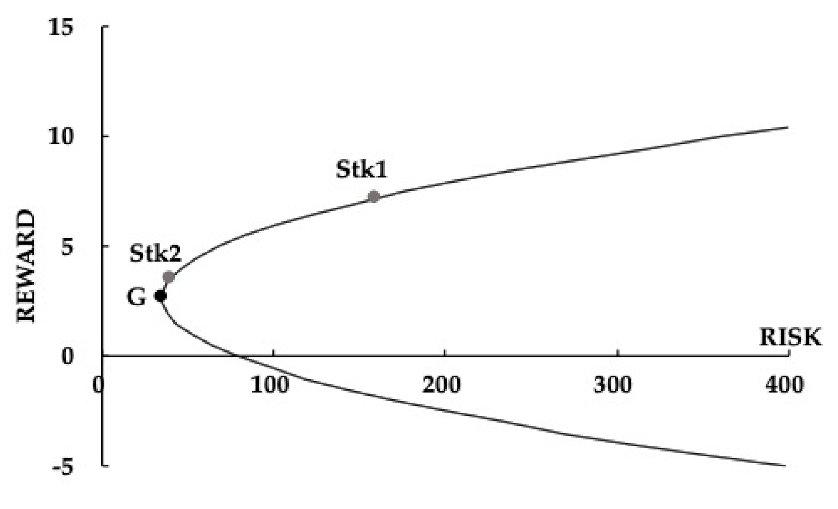
As Figure 1 shows, the coordinate of the annex $\mathit{G}$ of the portfolio frontier is $\left(1/c,b/c\right)$, and the risk and reward of the annex portfolio are $1/c$ and $b/c$, respectively. Note that the risk associated with portfolio $\mathit{G}$ is the lowest amongst all portfolios; hence it is called the global minimum risk portfolio (GMR portfolio). In the two-stock universe, any other portfolio bears a risk higher than $\mathit{G}$ does. Given the same risk level, portfolios located on the upper side always yield higher rewards than those on the lower side. Thus, the upper-sided frontier portfolios are called efficient portfolios. Corollary 1 shows that, for efficient portfolios, higher reward always accompanies higher risk, and the investment proportions change monotonically. Note that the efficiency ratio $d$ equals the ratio of ${\mu }_{\mathit{X}}-b/c$ to ${\sigma }_{\mathit{X}}^2-1/c$. For an N-asset economy, for any portfolio with a smaller reward or a bigger risk than a frontier portfolio $\mathit{X}$, its information ratio is apparently bigger than the efficiency ratio.

Corollary 1.

An efficient portfolio with higher risk is associated with a higher reward, and its investment proportion on a specific stock changes monotonically.

To a specific reward above $\mathit{G}$’s, the risk of the corresponding efficient portfolio is uniquely determined. In other words, the same efficient portfolio may be found by first specifying either its risk or reward.

Since portfolio $\mathit{G}$ bears the lowest risk globally, its risk level $1/c$ may be regarded as the reference for measuring opportunity risk, or the so-called excess risk, that is analogous to the concept of opportunity cost. Therefore, this particular portfolio may be regarded as the “benchmark portfolio” in the universe. Since $c=\mathbf{1}{\Sigma }^{-1}{\mathbf{1}}^{\prime }$, $\mathit{G}$’s risk is a function of stock risks and their corisk; that is, $\mathit{G}$’s risk has nothing to do with stock rewards! Furthermore, $\mathit{G}$’s reward is the ratio $b/c$. This is an interesting finding: “The unit disturbance determines $\mathit{G}$’s risk to $1/c$, while the ratio of the reward disturbance to unit risk determines the $\mathit{G}$’s reward to $b/c$.”

According to Lemma A4, the proportion of stock 1 in portfolio $\mathit{G}$ may be computed from Equation (8).

$${\alpha }_{\mathit{G}}=\frac{{\sigma }_2^2-{\sigma }_{12}}{{\sigma }_1^2-2{\sigma }_{12}+{\sigma }_2^2}$$

(8)

Unsurprisingly, there is no reward term in Equation (8); this confirms again that $\mathit{G}$’s stock composition is independent of stock rewards. Uniquely, through only the stock risks and corisk, one may determine the investment to construct the portfolio with global minimal risk.

As pointed out earlier in this section, the zero-reward portfolio is not an appropriate market reference against which other portfolios may be evaluated. The reference role could be better served by benchmark portfolio $\mathit{G}$. If portfolio $\mathit{G}$ is viewed as the performance benchmark, then a net reward above $\mathit{G}$ represents an excess reward, and net risk higher than $\mathit{G}$ represents excess risk. Thus, for portfolio $\mathit{X}$, its excess risk is ${\sigma }_{\mathit{X}}^2-1/c$ and excess reward is ${\mu }_{\mathit{X}}-b/c$, respectively.

The kernel $d$ of the Merton matrix is a constant. Thus, the kernel presents the optimal ratio of excess reward to excess risk; one may regard it as the optimal efficiency. Investors who choose not to act in accordance with Equation (7) will earn inferior reward at bearing a given level of risk. Investors with same required reward will choose the same efficient portfolio, so that the equilibrium is then reached in the two-stock market. Note that this relation holds only for rational investors, in the sense alluded to at the beginning of this paper.

To summarize, the market determines the benchmark portfolio $\mathit{G}$ solely on the basis of stock risks and their corisk, without any regard to their rewards whatsoever. The reward of $\mathit{G}$ may in turn be adopted as the reference for evaluating all portfolios. In order to achieve the optimal exchange between excess reward and excess risk, all rational investors will finally choose efficient portfolios. This implies that even though the security market involves only two stocks, as long as investors seek to achieve “optimal efficiency”, each risky asset will possess its own unique price.

According to Theorem 2, any portfolio on the frontier is a linear combination of any other two frontier portfolios, or the so-called “two-fund separation theory”. An important issue is therefore how these two key portfolios may be chosen.

Theorem 2.

Any frontier portfolio is a linear combination of any other two frontier portfolios.

Based on the proof in Theorem 2, if frontier portfolio $\mathit{X}$ owns reward ${\mu }_{\mathit{X}}$, then both $\mathit{X}$’s proportion vector and risk can be obtained by Equations (9) and (10), respectively.

$$\mathit{X}= \left({\mu }_{\mathit{X}},1\right)\mathit{B}$$

(9)

$${\sigma }_{\mathit{X}}^2= \left({\mu }_{\mathit{X}},1\right){\mathit{A}}^{-\mathbf{1}}\left(\begin{array}{c}{\mu }_{\mathit{X}}\\ \mathbf{1}\end{array}\right)$$

(10)

where $\mathit{B}={\mathit{A}}^{-\mathbf{1}}\left(\begin{array}{c}\mathit{\mu }\\ \mathbf{1}\end{array}\right){/\mathit{\Sigma }}^{-1}=\frac{1}{cd}\left(\begin{array}{c}c\mathit{\mu }-b\mathbf{1}\\ a\mathbf{1}-b\mathit{\mu }\end{array}\right){/\mathit{\Sigma }}^{-1}$ with the property $\mathit{B}/\mathit{\Sigma }{\mathit{B}}^{\prime }={\mathit{A}}^{-\mathbf{1}}$.

Observing Equation (9), it is clear that any frontier portfolio is a linear function of the stock reward vector $\mathit{\mu }$ and the one vector $\mathbf{1}$. Naturally, we may use each of these two vectors to construct two different funds. Due to $\mathbf{1}{\Sigma }^{-1}{\mathbf{1}}^{\prime }/c=$1, one knows that $\mathit{G}=1{\Sigma }^{-1}/c$ is the GMR portfolio. Specifically, $\mathit{G}$’s proportion vector is $\left({\sigma }_2^2-{\sigma }_{12},{\sigma }_1^2-{\sigma }_{12}\right)/cD$ and it owns reward $b/c$ and risk $1/c$. On the other hand, due to $\mathit{\mu }{\Sigma }^{-1}{\mathbf{1}}^{\prime }=b$, $\mathit{U}=\mathit{\mu }{\Sigma }^{-1}/b$ is indeed a portfolio. Specifically, the stock-reward portfolio $\mathit{U}$ owns the proportion vector $\left({\mu }_1{\sigma }_2^2-{\mu }_2{\sigma }_{12},{\mu }_2{\sigma }_1^2-{\mu }_1{\sigma }_{12}\right)/bD$ and one knows its reward $a/b$ and risk $a/b^2$ in use of Equations (1) and (2). On the other hand, this portfolio can be written as the equation $\mathit{U}=\left(a/b,1\right)\mathit{B}$. Substituting 0 for ${\mu }_X$ in Equation (8), one obtains the zero-reward portfolio $\mathit{O}=\left(0,1\right)\mathit{B}=\left(a\mathbf{1}-b\mathit{\mu }\right){\Sigma }^{-1}/cd$. Thus, $\mathit{O}=a\mathit{G}/d-b^2\mathit{U}/\mathrm{c}d$, that is, the zero-reward portfolio is a linear combination of portfolios $\mathit{G}$ and $\mathit{U}$. Substituting 1 for ${\mu }_X$ in Equation (8), one obtains the one-reward portfolio $\mathit{N}=\left(1,1\right)\mathit{B}=\left[\left(a-b\right)\mathbf{1}+\left(c-b\right)\mathit{\mu }\right]{\Sigma }^{-1}/cd$. Thus, $\mathit{N}=\left(a-b\right)\mathit{G}/d-b\left(c-b\right)\mathit{U}/\mathrm{c}d$, that is, the one-reward portfolio is a linear combination of portfolios $\mathit{G}$ and $\mathit{U}$ as well.

Define $\mathit{E}=\left(1,0\right)\mathit{B}$ as an error vector in the stock universe, specifically its proportion vector is $\left(c\mathit{\mu }-b\mathbf{1}\right){\Sigma }^{-1}/cd$. Due to proportions with zero-sum, the error vector is not a portfolio at all. For any frontier portfolio $\mathit{X}$ with rewards ${\mu }_{\mathit{X}}$, one has $\left({\mu }_{\mathit{X}},1\right)\mathit{B}=\left(0,1\right)\mathit{B}+{\mu }_{\mathit{X}}\left(1,0\right)\mathit{B}$, and then $\mathit{X}=\mathit{O}+{\mu }_{\mathit{X}}\mathit{E}$. Thus, Huang and Litzenberger [16] claimed that any frontier portfolio is a linear combination of the zero-reward portfolio and the error vector. Moreover, one may draw up the frontier envelope easily by using this linear combination with varying rewards.

The risks and corisk of the zero-reward portfolio $\mathit{O}$ and the error vector $\mathit{E}$ can be computed directly as below.

$$\mathit{O}\Sigma {\mathit{O}}^{\prime }=\left(0,1\right)\mathit{B}\Sigma {\mathit{B}}^{\prime }\left(\begin{array}{c}0\\ 1\end{array}\right)=\left(0,1\right)A^{-1}\left(\begin{array}{c}0\\ 1\end{array}\right)=\frac{a}{cd}$$

$$\mathit{E}\Sigma {\mathit{E}}^{\prime }=\left(1,0\right)\mathit{B}\Sigma {\mathit{B}}^{\prime }\left(\begin{array}{c}1\\ 0\end{array}\right)=\left(1,0\right)A^{-1}\left(\begin{array}{c}1\\ 0\end{array}\right)=\frac{1}{d}$$

$$\mathit{O}\Sigma {\mathit{E}}^{\prime }=\left(0,1\right)\mathit{B}\Sigma {\mathit{B}}^{\prime }\left(\begin{array}{c}1\\ 0\end{array}\right)=\left(0,1\right)A^{-1}\left(\begin{array}{c}1\\ 0\end{array}\right)=\frac{-b}{cd}$$

Furthermore, for a frontier $\mathit{X}$ with rewards ${\mu }_{\mathit{X}}$, its risk ${\sigma }_{\mathit{X}}^2$ can be computed directly as below.

$$\mathit{X}\Sigma {\mathit{X}}^{\prime }=\left(\mathit{O}+{\mu }_{\mathit{X}}\mathit{E}\right)\Sigma \left({\mathit{O}}^{\prime }+{\mu }_{\mathit{X}}{\mathit{E}}^{\prime }\right)=\left(a-2b{\mu }_{\mathit{X}}+c{\mu }_{\mathit{X}}^2\right)/cd$$

2.2. Portfolio Corisk

According to Equation (9), every frontier portfolio is a linear function of the one vector and the reward vector. By examining Equation (10) more closely, one may understand how the risk of a frontier portfolio is influenced by the stock rewards, stock risks and stocks’ corisk.

Theorem 3.

If $\mathit{X}$ and $\mathit{Y}$ are two frontier portfolios with rewards ${\mu }_{\mathit{X}}$ and ${\mu }_{\mathit{Y}}$, then their corisk is determined by Equation (11).

$${\sigma }_{\mathit{X}\mathit{Y}}=\frac{1}{c}+\frac{1}{d}\left({\mu }_{\mathit{X}}-\frac{b}{c}\right)\left({\mu }_{\mathit{Y}}-\frac{b}{c}\right)$$

(11)

According to the proof of Theorem 3, the corisk of these two frontier portfolios may be written in matrix form as Equation (12).

$${\sigma }_{\mathit{X}\mathit{Y}}=\left({\mu }_{\mathit{X}},1\right){\mathit{A}}^{-\mathbf{1}}\left(\begin{array}{c}{\mu }_{\mathit{Y}}\\ \mathbf{1}\end{array}\right)$$

(12)

Similar to Equation (7), relative to portfolio $\mathit{G}$, the multiplicands ${\mu }_{\mathit{X}}-b/c$ and ${\mu }_Y-b/c$ in Equation (11) are excess rewards of portfolios $\mathit{X}$ and $\mathit{Y}$, respectively. Therefore, for any two frontier portfolios, their corisk is determined by $1/c$ plus the product of two excess rewards adjusted by the efficiency ratio $d$. Next, one may prove that any two frontier portfolios on the same side have a positive corisk. If both portfolios are located on the upper side of the frontier, then both their excess rewards are positive and thus their product is positive as well. The positive argument also holds for lower side frontier portfolios, since the product of two negative excess rewards is positive. Equation (11) also implies that the corisk for two frontier portfolios on the same side increases with their reward difference.

Thus, two frontier portfolios that are negatively correlated must be located on the opposite sides of the frontier; however, the reverse is not necessarily true. Further examining the right-hand side of Equation (11), one may find that if the absolute value of the second term is not smaller than the first term, then the portfolios’ corisk remains positive. Therefore, the corisk of two frontier portfolios on the opposite sides may be positive, provided that the lower side portfolio is close enough to the GMR portfolio $\mathit{G}$ in order to insure that the absolute value of the product of excess rewards is still smaller than $1/c$.

Since any frontier portfolio is a linear combination of two other frontier portfolios, the reward of any convex frontier portfolio falls within these two known component portfolios. As short selling is allowed, a new portfolio located far above $\mathit{G}$ may potentially achieve much higher reward while its associated risk would be much higher as well.

It is known that $\mathit{G}=\mathbf{1}{\Sigma }^{-1}/c$; thus, for any portfolio $\mathit{X}$, the corisk is $\mathbf{1}{\Sigma }^{-1}\Sigma {\mathit{X}}^{\prime }/c=1/c$. This implies that the corisk of any portfolio with the $\mathit{G}$ equals $1/c$. Notably, this astonishing result indicates that the corisk of any portfolio and benchmark $\mathit{G}$ equals the $\mathit{G}$’s risk. This unique property of a constant corisk associated with $\mathit{G}$ invokes an interesting analogy. In optics, light rays beaming toward a parabolically-shaped mirror will all reflect from the mirror and pass through its focal point. Similarly, in the risk–reward space, the benchmark portfolio $\mathit{G}$ plays the role of “focusing” the pricing behavior of assets as well as portfolios.

By closely examining again Equation (11), one may discover more interesting phenomena. For instance, suppose one fixes a frontier portfolio on the upper side frontier, say portfolio $\mathit{P}$, and then tries to grasp the change of its corisk with another frontier portfolio $\mathit{Q}$. At the position of $\mathit{P}$, the corisk of the portfolio with itself is its own risk; return variance and the corisk decrease as the other portfolio $\mathit{Q}$ moves down toward portfolio $\mathit{G}$. As long as frontier portfolio $\mathit{Q}$ stays above portfolio $\mathit{G}$, its corisk with $\mathit{P}$ will be positive. Even if $\mathit{Q}$ moves down to a position somewhat lower than $\mathit{G}$, the corisk will still be positive. The corisk equals zero when that portfolio $\mathit{Q}$ reaches the zero-corisk position. After that point, the corisk turns negative as the portfolio $\mathit{Q}$ moves down below the zero-corisk position.

Now, one may turn attention to the issue regarding the corisk of a pure stock with a frontier portfolio. Without loss of generality, stock 1 and stock 2 may be viewed as two portfolios with proportion vectors $X_1=\left(1,0\right)$ and $X_2=\left(0,1\right)$. Thus, one may directly obtain Equation (13) for any frontier portfolio $\mathit{X}$.

$${\sigma }_{j\mathit{X}}=\left({\mu }_{\mathit{X}},1\right){\mathit{A}}^{-\mathbf{1}}\left(\begin{array}{c}{\mu }_j\\ 1\end{array}\right), j=1,2$$

(13)

One may expand Equation (13) to obtain Equation (14), which is in similar form as Equation (11). This equation expresses the corisk of a pure stock with a frontier portfolio $\mathit{X}$.

$${\sigma }_{j\mathit{X}}=\frac{1}{c}+\frac{1}{d}\left({\mu }_{\mathit{X}}-\frac{b}{c}\right)\left({\mu }_j-\frac{b}{c}\right), j=1,2$$

(14)

The quantities ${\mu }_{\mathit{X}}-b/c$ and ${\mu }_j-b/c$ in Equation (14) are both excess rewards. Hence it is apparent that the corisk of the pure stock with a frontier portfolio is determined by $\mathit{G}$’s risk $1/c$ plus the product of these two excess rewards adjusted by the efficiency ratio $d$. Now, one may summarize the above result in vector form as Equation (15). This implies that the corisk of the stocks with any frontier portfolio is a linear function of stocks’ reward vector.

$${\sigma }_{I\mathit{X}}=\left({\mu }_{\mathit{X}},1\right){\mathit{A}}^{-\mathbf{1}}\left(\begin{array}{c}\mathit{\mu }\\ \mathbf{1}\end{array}\right)$$

(15)

Corollary 2 extends the stock corisk with single frontier portfolio to a regression over two frontier portfolios.

Corollary 2.

If frontier portfolios $\mathit{X}$ and $\mathit{Y}$ have different rewards ${\mu }_{\mathit{X}}$ and ${\mu }_{\mathit{Y}}$, then the corisk vector of stocks may be shown as the regression model in Equation (16).

$${\mathit{\sigma }}_{\mathit{I}\mathit{X}}=\mathit{\alpha }{\sigma }_{\mathit{X}}^2+\left(1-\mathit{\alpha }\right){\sigma }_{\mathit{X}\mathit{Y}}$$

(16)

where$\mathit{\alpha }=\frac{1}{{\mu }_{\mathit{X}}-{\mu }_{\mathit{Y}}}\left(\mathit{\mu }-{\mathit{\mu }}_Y\mathbf{1}\right)$.

Thus, using Equation (16), one may find some stock’s corisk with portfolio $\mathit{X}$ by virtue of the regression relation as Equation (17).

$${\sigma }_{j\mathit{X}}={\alpha }_j{\sigma }_{\mathit{X}}^2+\left(1-{\alpha }_j\right){\sigma }_{\mathit{X}\mathit{Y}}, j=1,2$$

(17)

where ${\alpha }_j=\frac{{\mu }_j-{\mu }_{\mathit{Y}}}{{\mu }_{\mathit{X}}-{\mu }_{\mathit{Y}}}$.

Referring to any two different frontier portfolios, Corollary 2 shows that a pure stock may regress over one’s risk and their corisk. Therefore, by identifying two special frontier portfolios, one may employ Equation (17) to price pure stocks. If $\mathit{G}=\mathbf{1}{\Sigma }^{-1}/c$ and $\mathit{U}=\mathit{\mu }{\Sigma }^{-1}/b$ are the two chosen frontier portfolios, then the regression model degenerates to ${\sigma }_{j\mathit{G}}=1/c, j=1,2$. Thus, benchmark portfolio $\mathit{G}$ cannot appropriately play the spanning role. Due to ${\alpha }_j=b{\mu }_j/a$ and ${\sigma }_{\mathit{U}}^2=a/b^2$, if stock-reward portfolio $\mathit{U}$ and zero-reward portfolio $\mathit{O}$ are chosen, then the regression model gives the result below.

$${\sigma }_{j\mathit{U}}=\frac{1}{b}{\mu }_j+\left(1-\frac{b{\mu }_j}{c}\right){\sigma }_{\mathit{U}\mathit{O}}, j=1,2$$

which shows that the corisk of a pure stock to the reward portfolio is related to the reward of the stock in question.

3. Capital Asset Pricing Model

Since any frontier portfolio should be a linear combination of two other frontier portfolios, it is possible that a specific pair of portfolios play an important role in the pricing of risky assets. Note that these two portfolios should have zero corisk, that is, they need to be statistically orthogonal. Thus, the corisk regression Equation (17) for stocks has the degenerate form ${\sigma }_{j\mathit{X}}={\alpha }_j{\sigma }_{\mathit{X}}^2$. Since the corisk of benchmark portfolio $\mathit{G}$ with any portfolios is a positive constant, the GMR portfolio does not have any orthogonal portfolio.

Theorem 4.

For each portfolio $\mathit{Y}$ with reward ${\mu }_{\mathit{Y}}$ located on the lower side of the frontier, there exists a unique orthogonal portfolio $\mathit{X}$ with a reward and proportion vector shown below.

$${\mu }_{\mathit{X}}=\frac{a-b{\mu }_{\mathit{Y}}}{b-c{\mu }_{\mathit{Y}}}$$

(18)

$$\mathit{X}=\frac{1}{b-c{\mu }_{\mathit{Y}}}\left(\mathit{\mu }-{\mu }_{\mathit{Y}}\mathbf{1}\right){\Sigma }^{-1}$$

(19)

Once the reward of a lower side frontier portfolio is known, one may use Equations (9) and (10) to calculate its proportion vector and risk. Furthermore, one may use Equations (18) and (19) to compute the reward and then the proportion vector of its orthogonal portfolio. In use of Equation (19), one may find that stock-reward portfolio $\mathit{U}$ is orthogonal to zero-reward portfolio $\mathit{O}$. Due to lack of economic reason, this pair of reward orthogonal portfolios is not appropriate to play the role in the theorem of two funds’ separation.

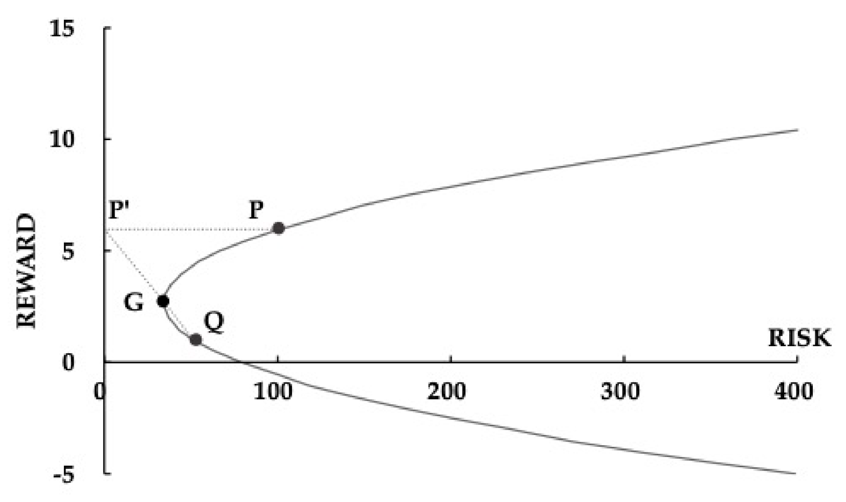
As shown in Figure 2 based on Lemma A6, in order to identify the frontier portfolio $\mathit{P}$ orthogonal to frontier portfolio $\mathit{Q}$, one may proceed as follows: (1) Draw a line passing through points $\mathit{Q}$ and $\mathit{G}$, which intersects the vertical axis at ${\mathit{P}}^{\prime }$; (2) draw a horizontal line from ${\mathit{P}}^{\prime }$ to the right, which intersects with the frontier at point $\mathit{P}$.

3.1. Market Portfolio

For the theory of two-fund separation, the frontier portfolio with reward equal to the risk-free interest rate is one choice, while the market portfolio is another. As stated in Theorem 4, any frontier portfolio located below the benchmark portfolio has a unique orthogonal portfolio located on the upper side of the frontier. Assume that investors adopt $R_f$, the risk-free interest rate, as their reward threshold. Further assume that the threshold portfolio $\mathit{Z}$ is the frontier portfolio with the reward equal to the threshold. Apparently, one may use Equation (9) to find $\mathit{Z}$’s proportion vector, i.e., $\mathit{Z}=\left(R_f,1\right)\mathit{B}$, and use Equation (10) to compute $\mathit{Z}$’s risk, namely ${\sigma }_{\mathit{Z}}^2=c{R}_f^2-2b{R}_f+a$.

Let $\mathit{M}$ be the portfolio orthogonal to the threshold portfolio $\mathit{Z}$, which is called the investors’ market portfolio. According to Theorem 4, portfolio $\mathit{M}$ is located on the upper side of the frontier. Applying Equation (19), one obtains $\mathit{M}$’s proportion vector $\left(\mathit{\mu }-R_f\mathbf{1}\right){\Sigma }^{-1}/\left(b-c{R}_f\right)$. Based on Lemmas A7 and A8, the reward and risk for portfolio $\mathit{M}$ may be written as flows:

$${\mu }_{\mathit{M}}=\frac{a-b{R}_f}{b-c{R}_f}$$

(20)

$${\sigma }_{\mathit{M}}^2=\frac{{\mu }_{\mathit{M}}-R_f}{b-c{R}_f}$$

(21)

Once the threshold and market portfolios are identified, any frontier portfolio can be written as a linear combination of these two key portfolios by virtue of Theorem 2. The economic implications of these two portfolios will be further addressed in the following paragraphs. If $\mathit{P}$ is a frontier portfolio with reward ${\mu }_{\mathit{P}}$, then investors may construct a bond–stock portfolio $\mathit{X}$ with proportion vector $\mathit{\alpha }=\left(\alpha ,1-\alpha \right)$ over bond and portfolio $\mathit{P}$, where bond offers threshold reward. The return of portfolio $\mathit{X}$ is the random variable ${\tilde{R}}_{\mathit{X}}=\alpha R_f+\left(1-\alpha \right){\tilde{R}}_{\mathit{P}}$, with reward $\alpha R_f+\left(1-\alpha \right){\mu }_{\mathit{P}}$ and risk ${\left(1-\alpha \right)}^2{\sigma }_{\mathit{P}}^2$. If an investor specifies κ as his/her acceptable level of reward for portfolio $\mathit{X}$, then the investment proportion on the bond is shown in Equation (22).

$$\alpha =\frac{{\mu }_{\mathit{P}}-\kappa }{{\mu }_{\mathit{P}}-R_f}$$

(22)

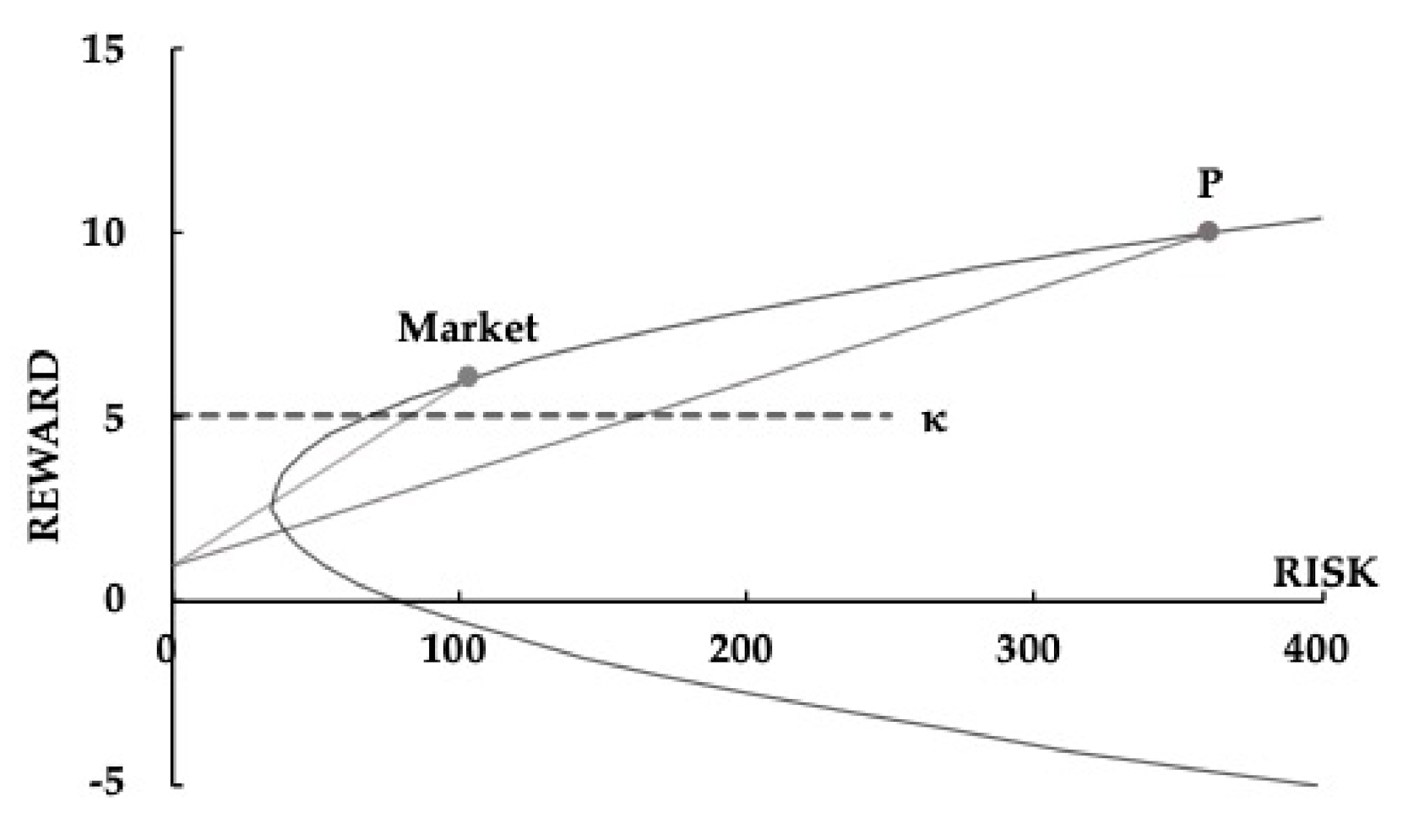
Theorem 5.

For all bond–stock portfolios with a same reward, the portfolio incorporating market portfolio as its stock portfolio has the lowest variance (the lowest risk).

Figure 3 allows one to compare quantitatively the riskiness of bond–stock portfolios with the same reward. Apparently, portfolio $\mathit{M}$ is capable of risk reduction for bond–stock portfolios. Thus, the theorem of two funds’ separation holds: “Regardless their preferences, all rational investors will choose a portfolio composed of the pair of threshold-reward orthogonal portfolios”.

3.2. CAPM

Now, the corisk between pure stocks and market portfolio $\mathit{M}$ will be investigated, which may be written as Equation (23) below by virtue of Lemma A9.

$${\sigma }_{j\mathit{M}}=\frac{{\mu }_j-R_f}{b-c{R}_f}, j=1,2$$

(23)

After examining Equations (20)–(23) altogether, one may find that the reward on pure stock is indeed related to $\mathit{M}$’s risk and reward as well as its corisk. Furthermore, based on Lemma A10, one may assert that the corisk between frontier portfolio $\mathit{P}$ and the market portfolio $\mathit{M}$ equals the right-hand side of Equation (24).

$${\sigma }_{\mathit{P}\mathit{M}}=\frac{{\mu }_{\mathit{P}}-R_f}{b-c{R}_f}$$

(24)

In order to price individual assets or portfolios, one must utilize their covariation with the market, which is typically embedded in the risk measure beta [8,12,17]. Define the beta coefficient as the corisk between a stock portfolio and the market portfolio, divided by the risk of the market. The portfolio betas may be written as ${\beta }_{\mathit{P}\mathit{M}}={\sigma }_{\mathit{P}\mathit{M}}/{\sigma }_{\mathit{M}}^2$, while pure stock betas may be written as ${\beta }_{j\mathit{M}}={\sigma }_{j\mathit{M}}/{\sigma }_{\mathit{M}}^2, j=1,2$. Apparently, the market portfolio has a unit beta, while the beta for its orthogonal portfolio, bond portfolio $\mathit{Z}$, is zero, or the so-called “zero-beta portfolio”.

Assume investors regard $R_f$ as the threshold reward. Dividing both sides of Equation (23) by the same sides of Equation (21), one obtains the beta for stock 1 and stock 2. After rearranging terms, this beta expression yields Equation (25) for stock 1 and stock 2. Note that this equation is just the famous CAPM. Alternatively, one may express the CAPM in matrix form for all stocks traded in the market as in Equation (26).

$${\mu }_j=R_f+{\beta }_{j\mathit{M}}\left({\mu }_{\mathit{M}}-R_f\right), j=1,2$$

(25)

$$\mathit{\mu }=R_f\mathbf{1}+\mathit{\beta }\left({\mu }_{\mathit{M}}-R_f\right)$$

(26)

The constant term ${\mu }_{\mathit{M}}-R_f$ in Equation (25) represents the excess reward relative to the threshold reward, which may be called the systematic reward. The term ${\beta }_{j\mathit{M}}\left({\mu }_{\mathit{M}}-R_f\right)$ may be regarded as the risk premium for stock j, since it reflects the extra reward investors required for bearing the risk as measured by the stock’s beta. Therefore, pure stock return equals investors’ threshold reward plus risk premium. In particular, since the beta for the market portfolio is 1, its risk premium should exactly equal ${\mu }_{\mathit{M}}-R_f$.

Once an investor has determined his/her threshold reward, the pair of orthogonal portfolios may be identified immediately, namely, the threshold portfolio and its associated market portfolio. Treating this pair as two mutual funds, investors could be better off in their own two-fund investment world by linearly combining these two funds.

Given the initial price $S_0$ of a stock and its beta with the market, investors may use Equation (25) to derive the expected end-of-period price $S_T$ for this stock.

$$S_T=S_0\left[R_f+\beta \left({\mu }_{\mathit{M}}-R_f\right)\right]$$

(27)

Rewriting Equation (26), one obtains Equation (28) for portfolios. In other words, investors will be able to price any portfolio once its beta is known.

$${\mathit{S}}_{\mathit{T}}={\mathit{S}}_{\mathbf{0}}\left[R_f\mathbf{1}+\mathit{\beta }\left({\mu }_{\mathit{M}}-R_f\right)\right]$$

(28)

One may re-write Equation (28) into Equation (29), which shows that the portfolio reward is the proportioned average over threshold reward and market reward, where the proportion is portfolio beta.

$${\mu }_{\mathit{P}}=\left(1-{\beta }_{\mathit{P}\mathit{M}}\right)R_f+{\beta }_{\mathit{P}\mathit{M}}{\mu }_{\mathit{M}}$$

(29)

3.3. Securities Market Line (SML)

In a two-dimensional world in which the horizontal and vertical axes represent beta and reward, respectively, the beta–reward line of Equation (28) is called the securities market line (SML). The threshold reward $R_f$ and the market risk premium ${\mu }_{\mathit{M}}-R_f$ represent respectively the intercept and slope of the SML. Since the market risk premium is positive in a rational world, a higher beta will entice a higher reward.

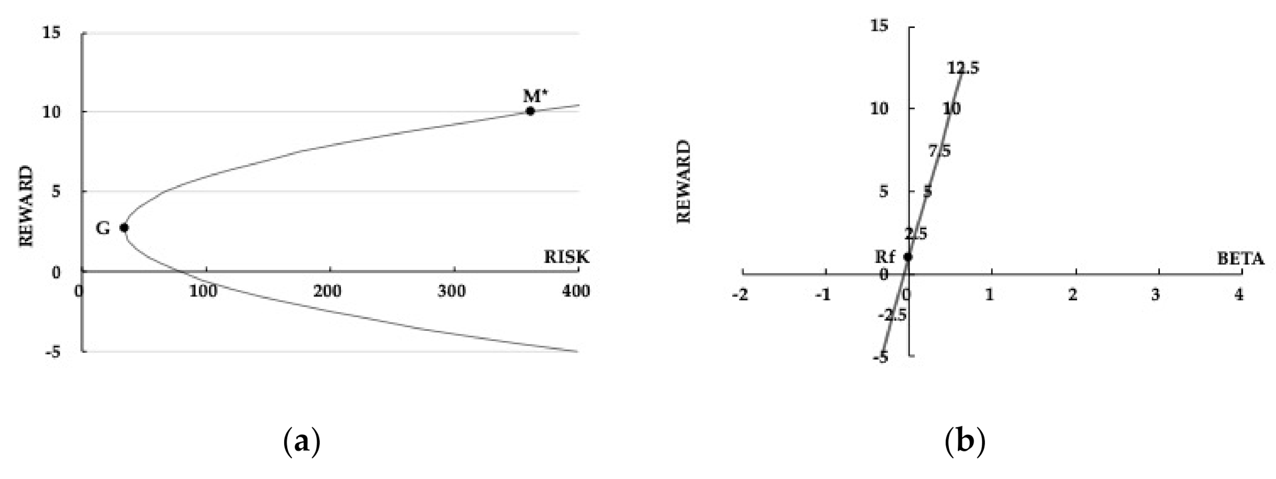
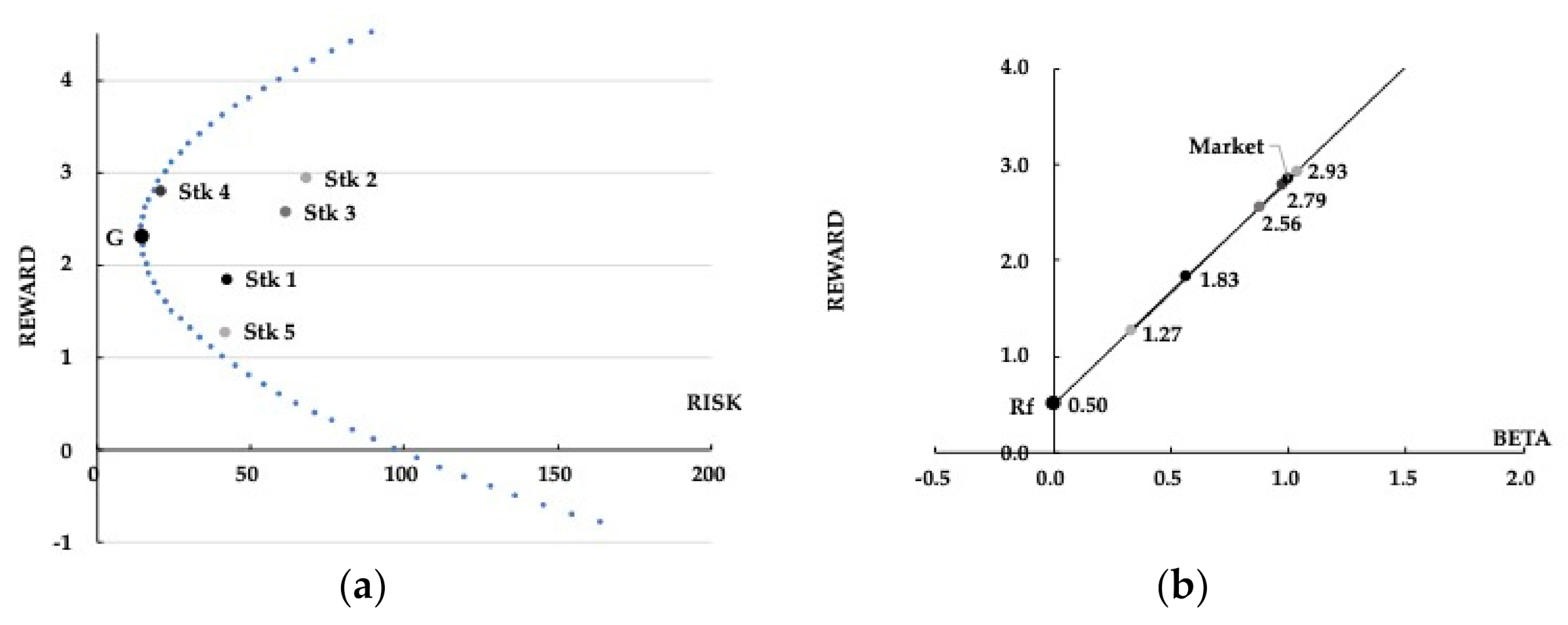
Assume investors have identified portfolio $\mathit{Z}$, located below the benchmark portfolio $\mathit{G}$, as their threshold portfolio with the least acceptable reward $R_f$. Furthermore, they have also identified the portfolio $\mathit{M}$, orthogonal to portfolio $\mathit{Z}$, as their market portfolio. Figure 4a exhibits how beta values change as a portfolio moves along the parabola frontier, relative to the market portfolio $\mathit{M}$. When the frontier portfolio is located far northeast to $\mathit{M}$, its beta is much higher than 1.0. Moving the portfolio northeast toward $\mathit{M}$, its beta will approach unity gradually. As the portfolio moves pass over $\mathit{M}$ but still remains above the benchmark portfolio $\mathit{G}$, its beta decreases to less than 1.0 but is still positive. As the portfolio moves closer to $\mathit{G}$, its beta approaches the risk ratio ${\beta }_{\mathit{G}\mathit{M}}=1/c{\sigma }_{\mathit{M}}^2$ of $\mathit{G}$ to $\mathit{M}$. Moving the portfolio to threshold $\mathit{Z}$, its beta decreases to zero exactly, and turns negative once the downward movement is past $\mathit{Z}$. In summary, portfolio beta monotonically decreases from positive to negative as portfolios move down along the frontier; upper-side betas are positively increasing with risk and lower-side betas are negatively decreasing with risk.

Figure 4b is a counterpart of Figure 4a. It displays the beta-reward relation for frontier portfolios. In Figure 4b, portfolios with higher betas are associated with higher rewards. Apparently, the beta-reward relation can be depicted by a straight line. The exercise of changing beta values moving down the frontier analyzed above may now be characterized more precisely as follows: (1) if ${\mu }_{\mathit{P}}>{\mu }_{\mathit{M}}$, then ${\sigma }_{\mathit{P}\mathit{M}}>{\sigma }_{\mathit{M}}^2$ and ${\beta }_{\mathit{P}\mathit{M}}>1$; (2) when ${\mu }_{\mathit{P}}={\mu }_{\mathit{M}}$, our deviation shows ${\sigma }_{\mathit{P}\mathit{M}}={\sigma }_{\mathit{M}}^2$ and ${\beta }_{\mathit{P}\mathit{M}}=1$; (3) if ${\mu }_{\mathit{G}}<{\mu }_{\mathit{P}}<{\mu }_{\mathit{M}}$, then ${\sigma }_{\mathit{P}\mathit{M}}>{\sigma }_{\mathit{G}}^2$ and $0<{\beta }_{\mathit{G}\mathit{M}}<{\beta }_{\mathit{P}\mathit{M}}<1\mathrm{are}\mathrm{found}$; (4) when ${\mu }_{\mathit{P}}={\mu }_{\mathit{G}}$, we show that ${\sigma }_{\mathit{P}\mathit{M}}<{\sigma }_{\mathit{M}}^2$ and $0<{\beta }_{\mathit{G}\mathit{M}}={\beta }_{\mathit{P}\mathit{M}}<1$; (5) if ${\mu }_{\mathit{G}}<{\mu }_{\mathit{P}}<{\mu }_{\mathit{M}}$, the evidence shows that ${\sigma }_{\mathit{P}\mathit{M}}>{\sigma }_{\mathit{G}}^2$ and $0<{\beta }_{\mathit{G}\mathit{M}}<{\beta }_{\mathit{P}\mathit{M}}<1$; (6) when ${\mu }_{\mathit{P}}={\mu }_{\mathit{Z}}$, then ${\sigma }_{\mathit{P}\mathit{M}}=0$ and $0={\beta }_{\mathit{P}\mathit{M}}<{\beta }_{\mathit{G}\mathit{M}}$; and (7) if ${\mu }_{\mathit{P}}<{\mu }_{\mathit{Z}}$, then the evidence of ${\sigma }_{\mathit{P}\mathit{M}}<0$ and ${\beta }_{\mathit{P}\mathit{M}}<0$ are found.

Suppose some investors specify a stricter threshold. As illustrated in Figure 5, the orthogonal pair of portfolios ${\mathit{Z}}^{*}$ and ${\mathit{M}}^{*}$ is chosen, which are located at the parabola higher than the old pair of portfolios $\mathit{Z}$ and $\mathit{M}$. Do these two groups of investors give different prices for the same stock as well as the same portfolio?

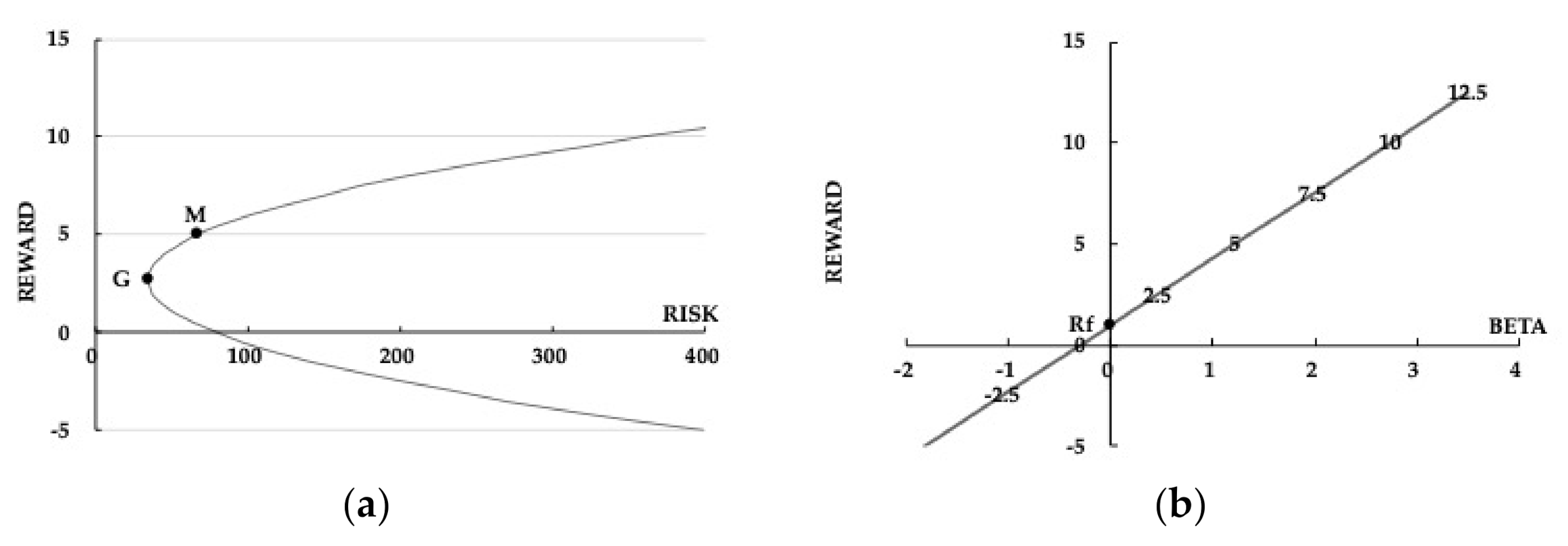
As shown in Figure 6a, the new ${\mathit{Z}}^{*}$ and ${\mathit{M}}^{*}$ are located higher, resulting in higher new betas for the same set of frontier portfolios. However, the terms on the left-hand side of Equations (24) and (28) will not change. Thus, regardless of the threshold reward chosen, investors will not price stocks and portfolios differently. As illustrated in Figure 6b, the new SML indeed is steeper, despite there being no reward change to the frontier portfolios.

Theorem 6.

Regardless of the threshold reward chosen, investors will not price stocks and portfolios differently.

According to Prospect Theory, investors use an S-shape value function in evaluating a prospect. Since the determination of capital gain and loss is crucial to assigning values, a wealth reference for prospect assessment is needed. In other words, the choice of the reference basis is highly personal, catering to the investor’s idiosyncratic needs. Now, the incorporation of the concept regarding prospect gain and loss into the risk–reward universe will proceed as follows. Relative to the threshold reward, one may regard the positive and negative systematic rewards as prospect gain and loss, respectively. As such, betas for the same portfolio may differ from person to person due to different threshold rewards. Although investors may have different threshold rewards, this paper demonstrates the “identical-pricing” implication arising from the CAPM.

4. Empirical Analysis

4.1. Empirical Results for Two Stocks

For the purpose of numerical demonstration throughout this paper, we acquired the US equity from the period of July 2016 to June 2021 from Yahoo Finance. In the two stocks world, we selected two high-listed liquidity stocks of major American companies, Amazon (AMZN) and Starbucks (SBUX). Their monthly rewards and standard deviations are in percentage, say ${\mu }_1=2.56$, ${\mu }_2=1.27$, and ${\sigma }_1=7.87$, ${\sigma }_2=6.51,$ with the correlation coefficient ${\rho }_{12}=0.20$. Thus, the securities universe owns the reward vector $\mathit{\mu }=\left(2.56, 1.27\right)$ and reward difference $\Delta =1.29$, as well as the corisk matrix exhibited below.

$$\Sigma =\left(\begin{array}{cc}61.97& 10.19\\ 10.19& 42.33\end{array}\right),\mathrm{with}\mathrm{determinant}\mathrm{D}=2519.39.$$

Assume that the shares of these two stocks may be divided into infinitesimal units. Let $\mathit{X}$ be a linear combination of stock 1 and stock 2 with proportion vector $\left(\alpha ,1-\alpha \right)$. Then the proportion on stock 1 is shown as Equation (4). Suppose portfolios $\mathit{X}=\left(0.6, 0.4\right)$ and $\mathit{Y}=\left(0.4, 0.6\right)$, then the portfolio rewards are ${\mu }_{\mathit{X}}=2.05$ and ${\mu }_{\mathit{Y}}=1.79$ based on Equation (1), and the portfolio risks are ${\sigma }_{\mathit{X}}^2=33.97$ and ${\sigma }_{\mathit{Y}}^2=30.04$ based on Equation (2). The corisk ${\sigma }_{\mathit{X}\mathit{Y}}=30.33$ may be calculated based on Equation (3).

Let $\mathbf{1}=\left(1,1\right)$ be the one vector and then following Merton define $\mathit{A}$ as the information matrix of the securities universe as below:

$$\mathit{A}=\left(\begin{array}{cc}{\mu }_1& {\mu }_2\\ 1& 1\end{array}\right){\Sigma }^{-1}\left(\begin{array}{cc}{\mu }_1& 1\\ {\mu }_2& 1\end{array}\right)=\left(\begin{array}{c}\mathit{\mu }\\ \mathbf{1}\end{array}\right){\Sigma }^{-1}\left({\mathit{\mu }}^{\prime } ,\mathbf{1}\prime \right)\mathrm{with}\mathrm{inverse}{\mathit{A}}^{-1}=\frac{1}{ac-b^2}\left(\begin{array}{cc}+c& -b\\ -b& +a\end{array}\right)$$

where $\mathit{A}$ owns elements $a_{11}=a=\mathit{\mu }{\Sigma }^{\prime }{\mathit{\mu }}^{\prime }$, $a_{12}=a_{21}=b=\mathit{\mu }{\Sigma }^{-1}{\mathbf{1}}^{\prime }$, and $a_{22}=c=\mathbf{1}{\Sigma }^{-1}{\mathbf{1}}^{\prime }$. We then have the elements $a=0.1238$, $b=0.0589$, $c=0.0333$, and $d=0.0197$. Moreover, if investors specify a reward level ${\mu }_{\mathit{X}}$, we can use Equation (4) to acquire stock proportions, and use Equation (6) to calculate its associated risk. In case of zero reward, the zero-reward portfolio $\mathit{O}$ has (−0.99, 1.99) as its proportion vector and its risk is 188.84, whereas if the reward is specified as 1.6 percent, then one has the portfolio proportions 0.25 and 0.75 on stock 1 and stock 2, respectively, and the risk is 31.45. In the two-stock universe, using Equation (8), the proportions of stock 1 and stock 2 in the global GMR portfolio $\mathit{G}$ are 0.38 and 0.62, respectively.

Based on Theorem 2, if frontier portfolio $\mathit{X}$ owns reward ${\mu }_{\mathit{X}}$, then both $\mathit{X}$’s proportion vector and risk can be obtained by Equations (9) and (10), respectively. For example, GMR portfolio $\mathit{G}$(0.38, 0.62) incurs a risk of 30.02 and a reward of 1.77 percent, while $\mathit{U}\left(0.25, 0.75\right)$ incurs a risk 31.45 and reward of 1.6 percent; on the other hand, the zero-reward portfolio $\mathit{O}=6.27\mathit{G}-5.27\mathit{U}$ incurs a risk of 188.84, which is greater than the risks of both portfolios $\mathit{G}$ and $\mathit{U}$. However, for the error vector $\mathit{E}=\left(1,0\right)\mathit{B}=\left(0.777,-0.777\right)$ with the position of long stock 1 and short stock 2, if there is a frontier portfolio $\mathit{X}$ with a reward of 1.4 percent, then the proportion vector $\mathit{X}=\mathit{O}+1.4\mathit{E}=\left(0.1,0.9\right)$.

According to Theorem 3, if $\mathit{X}$ and $\mathit{Y}$ are two frontier portfolios with rewards ${\mu }_{\mathit{X}}$ and ${\mu }_{\mathit{Y}}$, then their corisk is determined by Equation (11). If the frontier portfolios $\mathit{X}$(2.89, −1.89) and $\mathit{O}$(−0.99, 1.99) are chosen, then we have ${\mu }_{\mathit{X}}=5.0$, ${\mu }_0=0.0$, ${\sigma }_{\mathit{X}}^2=559.27$ and ${\sigma }_{\mathit{X}\mathbf{0}}=-259.45$. Moreover, following Corollary 2 and using Equation (17), we can find the proportion ${\alpha }_1=0.512$ and that the corisk of stock 1 with $\mathit{X}$ is ${\sigma }_{\mathbf{1}\mathit{X}}$ = 0.512 × 559.27 + 0.488 × (−259.45) = 160.05. Similarly, since ${\alpha }_2=0.255$, the corisk ${\sigma }_{\mathbf{2}\mathit{X}}$ of stock 2 equals 0.255 × 559.27 + 0.745 × (−259.45) = −50.70.

If we assume that investors adopt the default-free bond with $R_f=1.0$ percent and the risk-free interest rate, as their reward threshold there will be a frontier portfolio $\mathit{Z}$ with the reward equal to the threshold, which has the proportion vector (−0.21, 1.21) and a risk of 59.89. Since any frontier portfolio should be a linear combination of other two frontier portfolios, there will be a portfolio $\mathit{M}$ orthogonal to the threshold portfolio $\mathit{Z}$, which is called an investors’ market portfolio. Using Equations (20) and (21), the market portfolio $\mathit{M}$ has a reward of 2.54 percent and a risk of 60.20 with the proportion (0.98, 0.02). For a frontier proportion $P\left(2.00,-1.00\right)$ there is a reward of 3.85 percent and a risk of 249.66. Suppose that investors specify 2.0 percent for the required κ; following Theorem 5 and using Equation (22), investors may construct the bond–stock portfolio $\mathit{B}\mathit{S}$ with the proportions 0.65 of stock portfolio $\mathit{P}$ and 0.35 of bond portfolio $\mathit{Z}$, while $\mathit{B}\mathit{S}$’s risk is 0.65 × 249.66 = 162.28. On the other hand, the investor may construct another bond–stock portfolio $\mathit{B}\mathit{M}$ with the proportions 0.35 of market portfolio $\mathit{M}$ and 0.65 of bond portfolio $\mathit{Z}$, making $\mathit{B}\mathit{M}$’s risk 0.35 × 60.20 = 21.07 only. Moreover, for the pure stocks and market portfolio, the rewards of stock 1 and stock 2 are already known as ${\mu }_1=2.56$ percent and ${\mu }_2=1.27$ percent, respectively. Suppose that an investor specifies his/her threshold reward to be 1.0. For pure stock 1 and stock 2, because the pure stock betas can be written as ${\beta }_{j\mathit{M}}={\sigma }_{j\mathit{M}}/{\sigma }_{\mathit{M}}^2$, this investor can calculate the stock betas to be 1.014 and 0.179, respectively. Thus, the CAPM for this investor is as follows:

$${\mu }_{1\mathit{A}}=1+1.014\times \left(2.54-1.00\right)\mathrm{and}{\mu }_{2\mathit{A}}=1+0.179\times \left(2.54-1.00\right).$$

Here an interesting result emerges: “No matter what level of threshold rewards investors choose, the price of a pure stock as evaluated by the various CAPM mechanisms is identical across investors.” Consequently, the price for a stock portfolio produced by these CAPM mechanisms is identical across investors as well.

4.2. Empirical Results for Five Stocks

Using the same expressions as in Section 4.1, in this section, we calculate and trace out a Merton’s parabola and SML for five high liquidity stocks, including Nike (NKE), Apple (AAPL), Amazon (AMZN), Microsoft (MSFT), and Starbucks (SBUX).

Table 1. Summary Statistics for Stock Return.

	Mean	Median	Stk 1	Stk 2	Stk 3	Stk 4	Stk 5
Stk 1	1.828	1.506	42.856	17.922	16.783	10.419	8.774
Stk 2	2.928	4.664	17.922	68.755	36.795	24.364	11.736
Stk 3	2.562	2.584	16.783	36.795	61.966	26.932	10.188
Stk 4	2.790	2.777	10.419	24.364	26.932	21.129	8.511
Stk 5	1.275	1.629	8.774	11.736	10.188	8.511	42.333

Note: Percentage of monthly stock returns from July 2016 to June 2021, including mean, median and covariance matrix. Stk 1, 2, 3, 4, and 5 are NKE, AAPL, AMZN, MSFT, and SBUX, respectively.

shows the mean, median, and covariance matrix for the five stocks’ rewards. In Figure 7a,b, we extend the two-stocks universe to the five-stocks universe and depict the portfolio frontier and securities market line, respectively. In fact, this paper demonstrates that the major aspects of Merton’s derivation of the CAPM for a universe of N assets may also be obtained in a two-asset world.

5. Conclusions

By employing basic algebra, geometry, and statistics and invoking the risk aversion criterion, this paper successfully constructs the CAPM with two stocks only. Due to the vector-matrix approach, all main derivations in this paper can be easily extended to an N-security economy. There are four investment principles that students need to grasp through this paper. First, investors prefer less risk to more, and they prefer more reward to less. Second, investors possess homogeneous ex ante stock rewards, stock risks and corisks regarding the stocks within the confines of their securities universe. Third, investors may regard the risk-free rate of return as one choice of their reward threshold. Finally, the two-fund separation theorem holds due to the orthogonality between the threshold and the market portfolios.

Even starting with only two assets, investors are capable of establishing pricing relationship solely on the basis of ex ante rewards, risks and corisks. The risk of the benchmark portfolio is determined only by stock risks and their corisks, which is irrelevant to stock rewards. Thus, both excess risk and excess reward of a stock portfolio are accounted for relative to the benchmark portfolio. Furthermore, the portfolio frontier is a parabola in the risk–reward space consisting of all portfolios with an efficient tradeoff between excess risks to excess rewards.

To derive CAPM, two orthogonal spanning funds are crucial. The first one is the frontier portfolio with a reward equal to a default-free bond. The second portfolio is the market portfolio, which is orthogonal to the threshold portfolio. Exploiting a regression of stock corisks to the market portfolio, CAPM emerges naturally in this paper. In the case of a no default-free bond, CAPM still holds if investors specify their threshold reward to be the risk-free interest rate. Conceptually, the specified threshold plays the role of distinguishing gain or loss among prospects, which is advocated by Kahneman and Tversky. Furthermore, this paper illustrates one important implication of the pair of threshold portfolio and the market portfolio: even if investors start with a different pair of orthogonal frontier portfolios, they will not price assets and portfolios differently.

With respect to theoretical implications, our proofs shows that: (1) Personal recognition of the prospective gain/loss does not affect the stock pricing as well as portfolios; (2) we echo Somerville and O’Connell’s [2] findings that beta coefficients are endogenous in the mean-variance space; furthermore, we find that when the risk-free return exceeds the investor’s portfolio return, the beta of the portfolio will be negative; (3) the derivation of CAPM may be accomplished with STEM students’ undergraduate level of mathematic tools, which is beneficial to novices in this field; (4) both economic interpretations for CAPM and vector-matrix proofs are applicable to the N-stock economy. While finance is the study of financial decision making, “learning by doing” in universities’ finance teaching increasingly includes working with data. Our study has practical implications that are useful for financial educators who are concerned with incorporating emerging tools into instruction. Our expressions should be easily adopted by pre-finance graduate STEM students at the undergraduate mathematic level with our hand-on worksheets.

6. Future Research Directions and Limitations

Grinold and Kahn [18] mentioned the CAPM’s assumption that expected residual returns are zero, implying that passive investing is optimal. Many optimization techniques are used to manage passive funds. We believe that understanding vector-matrix expressions in this study will help STEM students learn more advanced portfolio construction models, such as Jorion’s [19] tracking-error constraints model. Based on CAPM, the future research should consider the effects of tracking error constraints on portfolio management teaching in the graduate school level. With respect to research limitations, in this study, the deep comprehension of CAPM circumvents teachers from suffering the tautology issues raised by Roll’s [9] critique.