Principal Bundle Structure of Matrix Manifolds

Abstract

In this paper, we introduce a new geometric description of the manifolds of matrices of fixed rank. The starting point is a geometric description of the Grassmann manifold ${\mathbb{G}}_r\left({\mathbb{R}}^k\right)$ of linear subspaces of dimension $r<k$ in ${\mathbb{R}}^k$, which avoids the use of equivalence classes. The set ${\mathbb{G}}_r\left({\mathbb{R}}^k\right)$ is equipped with an atlas, which provides it with the structure of an analytic manifold modeled on ${\mathbb{R}}^{(k-r)\times r}$. Then, we define an atlas for the set ${\mathcal{M}}_r\left({\mathbb{R}}^{k\times r}\right)$ of full rank matrices and prove that the resulting manifold is an analytic principal bundle with base ${\mathbb{G}}_r\left({\mathbb{R}}^k\right)$ and typical fibre ${\mathrm{GL}}_r$, the general linear group of invertible matrices in ${\mathbb{R}}^{k\times k}$. Finally, we define an atlas for the set ${\mathcal{M}}_r\left({\mathbb{R}}^{n\times m}\right)$ of non-full rank matrices and prove that the resulting manifold is an analytic principal bundle with base ${\mathbb{G}}_r\left({\mathbb{R}}^n\right)\times {\mathbb{G}}_r\left({\mathbb{R}}^m\right)$ and typical fibre ${\mathrm{GL}}_r$. The atlas of ${\mathcal{M}}_r\left({\mathbb{R}}^{n\times m}\right)$ is indexed on the manifold itself, which allows a natural definition of a neighbourhood for a given matrix, this neighbourhood being proved to possess the structure of a Lie group. Moreover, the set ${\mathcal{M}}_r\left({\mathbb{R}}^{n\times m}\right)$ equipped with the topology induced by the atlas is proven to be an embedded submanifold of the matrix space ${\mathbb{R}}^{n\times m}$ equipped with the subspace topology. The proposed geometric description then results in a description of the matrix space ${\mathbb{R}}^{n\times m}$, seen as the union of manifolds ${\mathcal{M}}_r\left({\mathbb{R}}^{n\times m}\right)$, as an analytic manifold equipped with a topology for which the matrix rank is a continuous map.

1. Introduction

Low-rank matrices appear in many applications involving high-dimensional data. Low-rank models are commonly used in statistics, machine learning or data analysis (see [1] for a recent survey). Furthermore, low-rank approximation of matrices is the cornerstone of many modern numerical methods for high-dimensional problems in computational science, such as model-order-reduction methods for dynamical systems or parameter-dependent or stochastic equations [2,3,4,5].

These applications yield problems of approximation or optimization in the sets of matrices with fixed rank:

$${\mathcal{M}}_r\left({\mathbb{R}}^{n\times m}\right)=\{Z\in {\mathbb{R}}^{n\times m}:\mathrm{rank}\left(Z\right)=r\}.$$

Fixed-rank matrices appear also in the theory of characteristics of Partial Differential Equations and Monge-Ampère equations [6]. More precisely, it has been proven [6,7] that Monge-Ampère equations with n independent variables and of Goursat-type are in one-to-one correspondence with the set $\{Z\in {\mathcal{M}}_r\left({\mathbb{R}}^{n\times n}\right):r\le 2\}.$ Thus, the parabolic or hyperbolic nature of the Monge-Ampère equation is related to the rank of such matrices.

In [8,9], the authors point out that Algebraic Geometry appears as a natural tool in study of the set ${\mathcal{M}}_r\left({\mathbb{R}}^{n\times m}\right).$ We wish to mention the papers [10,11,12] that raise the natural question of how large these matrix spaces are.

A usual geometric approach is to endow the set ${\mathcal{M}}_r\left({\mathbb{R}}^{n\times m}\right)$ with the structure of a Riemannian manifold [13,14], which is seen as an embedded submanifold of ${\mathbb{R}}^{n\times m}$ equipped with the topology ${\tau }_{{\mathbb{R}}^{n\times m}}$ given by matrix norms. Standard algorithms then work in the ambient matrix space ${\mathbb{R}}^{n\times m}$ and do not rely on an explicit geometric description of the manifold using local charts (see, e.g., [15,16,17,18]). However, the matrix rank considered as a map is not continuous for the topology ${\tau }_{{\mathbb{R}}^{n\times m}}$, which can yield undesirable numerical issues.

The purpose of this paper is to propose a new geometric description of the sets of matrices with fixed rank, which is amenable for numerical use, and relies on the natural parametrization of matrices in ${\mathcal{M}}_r\left({\mathbb{R}}^{n\times m}\right)$ given by

$$\begin{array}{c}\hfill Z=UG{V}^T,\end{array}$$

(1)

where $U\in {\mathbb{R}}^{n\times r}$ and $V\in {\mathbb{R}}^{m\times r}$ are matrices with full rank $r<min\{n,m\}$ and $G\in {\mathbb{R}}^{r\times r}$ is a non singular matrix. The set ${\mathcal{M}}_r\left({\mathbb{R}}^{n\times m}\right)$ is here endowed with the structure of analytic principal bundle with an explicit description of local charts. This results in a description of the matrix space ${\mathbb{R}}^{n\times m}$ as an analytic manifold with a topology induced by local charts that is different from ${\tau }_{{\mathbb{R}}^{n\times m}}$ and for which the rank is a continuous map. Note that the representation (1) of a matrix Z is not unique because $Z=\left(UP\right)\left(P^{-1}G{P}^T\right){\left(V{P}^{-1}\right)}^T$ holds for every invertible matrix P in ${\mathbb{R}}^{r\times r}$. An argument used to dodge this undesirable property is the possibility to uniquely define a tangent space (see for example Section 2.1 in [18]), which is a prerequisite for standard algorithms on differentiable manifolds. The geometric description proposed in this paper avoids this undesirable property. Indeed, the system of local charts for the set ${\mathcal{M}}_r\left({\mathbb{R}}^{n\times m}\right)$ is indexed on the set itself. This allows a natural definition of a neighbourhood for a matrix where all matrices admit a unique representation.

The present work opens the route for new numerical methods for optimization and dynamical low-rank approximation with algorithms working in local coordinates and avoiding the use of a Riemannian structure. In [19], such a framework is introduced for generalising iterative methods in optimization from Euclidean space to manifolds, which ensures that local convergence rates are preserved. Recently, a splitting algorithm relying on the geometric description of the set of fixed rank matrices proposed in this paper has been introduced for dynamical low-rank approximation [20].

The introduction of a principal bundle representation of matrix manifolds is also motivated by the importance of this geometric structure in the concept of gauge potential in physics [21].

Note that the proposed geometric description has a natural extension to the case of fixed-rank operators on infinite dimensional spaces and is consistent with the geometric description of manifolds of tensors with fixed rank proposed by Falcó, Hackbush and Nouy [22] in a tensor Banach space framework.

Before introducing the main results and outline of the paper, we recall some elements of geometry.

1.1. Elements of Geometry

In this paper, we follow the approach of Serge Lang [23] for the definition of a manifold $\mathbb{M}$. In this framework, a set $\mathbb{M}$ is equipped with an atlas which gives $\mathbb{M}$ the structure of a topological space, with a topology induced by local charts, and the structure of differentiable manifold compatible with this topology. More precisely, the starting point is the definition of a collection of non-empty subsets $U_{\alpha }\subset \mathbb{M}$, with $\alpha$ in a set A, such that ${\left\{U_{\alpha }\right\}}_{\alpha \in A}$ is a covering of $\mathbb{M}$. The next step is the explicit construction for any $\alpha \in A$ of a local chart ${\phi }_{\alpha }$ which is a bijection from $U_{\alpha }$ to an open set $X_{\alpha }$ of the finite dimensional space ${\mathbb{R}}^{N_{\alpha }}$ such that for any pair $\alpha ,{\alpha }^{\prime }\in \mathbb{M}$ such that $U_{\alpha }\cap U_{{\alpha }^{\prime }}\ne \varnothing$, the following properties hold:

(i)

${\phi }_{\alpha }(U_{\alpha }\cap U_{{\alpha }^{\prime }})$ and ${\phi }_{{\alpha }^{\prime }}(U_{\alpha }\cap U_{{\alpha }^{\prime }})$ are open sets in $X_{\alpha }$ and $X_{{\alpha }^{\prime }}$ respectively, and

(ii)

the map

$${\phi }_{{\alpha }^{\prime }}\circ {\phi }_{\alpha }^{-1}:{\phi }_{\alpha }(U_{\alpha }\cap U_{{\alpha }^{\prime }})⟶{\phi }_{{\alpha }^{\prime }}(U_{\alpha }\cap U_{{\alpha }^{\prime }})$$

is a $C^p$ differentiable diffeomorphism, with $p\in \mathbb{N}\cup \{\infty \}$ or $p=\omega$ when the map is analytic.

Under the above assumptions, the set $\mathcal{A}:=\{(U_{\alpha },{\phi }_{\alpha }):\alpha \in A\}$ is an atlas which endows $\mathbb{M}$ with a structure of $C^p$ manifold. Then, we can say that $(\mathbb{M},\mathcal{A})$ is a $C^p$ manifold, or an analytic manifold when $p=\omega$. A consequence of condition $\left(ii\right)$ is that when $U_{\alpha }\cap U_{{\alpha }^{\prime }}\ne \varnothing$ holds for $\alpha ,{\alpha }^{\prime }\in A$, then $N_{\alpha }=N_{{\alpha }^{\prime }}.$ In the particular case where $N_{\alpha }=N$ for all $\alpha \in A$, we say that $(\mathbb{M},\mathcal{A})$ is a $C^p$ manifold modelled on ${\mathbb{R}}^N.$ Otherwise, we say that it is a manifold not modelled on a particular finite-dimensional space. A paradigmatic example is the Grassmann manifold $\mathbb{G}\left({\mathbb{R}}^k\right)$ of all linear subspaces of ${\mathbb{R}}^k$, such that

$$\mathbb{G}\left({\mathbb{R}}^k\right)=\bigcup _{0\le r\le k}{\mathbb{G}}_r\left({\mathbb{R}}^k\right),$$

where ${\mathbb{G}}_0\left({\mathbb{R}}^k\right)=\left\{0\right\}$ and ${\mathbb{G}}_k\left({\mathbb{R}}^k\right)=\left\{{\mathbb{R}}^k\right\}$ are trivial manifolds and ${\mathbb{G}}_r\left({\mathbb{R}}^k\right)$ is a manifold modelled on the linear space ${\mathbb{R}}^{(k-r)\times r}$ for $0<r<k.$ Consequently, $\mathbb{G}\left({\mathbb{R}}^k\right)$ is a manifold not modelled on a particular finite-dimensional space.

The atlas also endows $\mathbb{M}$ with a topology given by

$${\tau }_{\mathcal{A}}:=\left\{{\phi }_{\alpha }^{-1}\left(O\right):\alpha \in A\mathrm{and}O\mathrm{an}\mathrm{open}\mathrm{set}\mathrm{in}{X}_{\alpha }\right\},$$

which makes $(\mathbb{M},{\tau }_{\mathcal{A}})$ a topological space where each local chart

$${\phi }_{\alpha }:(U_{\alpha },{\tau }_{\mathcal{A}}{|}_{U_{\alpha }})⟶(X_{\alpha },{\tau }_{{\mathbb{R}}^{N_{\alpha }}}{|}_{X_{\alpha }}),$$

considered as a map between topological spaces is a homeomorphism. (Here $(\mathfrak{X},\tau )$ denotes a topological space, and if ${\mathfrak{X}}^{\prime }\subset \mathfrak{X}$, then ${\tau |}_{{\mathfrak{X}}^{\prime }}$ denotes the subspace topology.)

1.2. Main Results and Outline

Our first remark is that the matrix space ${\mathbb{R}}^{n\times m}$ is an analytic manifold modelled on itself, and its geometric structure is fully compatible with the topology ${\tau }_{{\mathbb{R}}^{n\times m}}$ induced by a matrix norm. In this paper, we define an atlas on ${\mathcal{M}}_r\left({\mathbb{R}}^{n\times m}\right)$, which gives this set the structure of an analytic manifold, with a topology induced by the atlas fully compatible with the subspace topology ${\tau }_{{\mathbb{R}}^{n\times m}}{|}_{{\mathcal{M}}_r\left({\mathbb{R}}^{n\times m}\right)}$. This implies that ${\mathcal{M}}_r\left({\mathbb{R}}^{n\times m}\right)$ is an embedded submanifold of the matrix manifold ${\mathbb{R}}^{n\times m}$ modelled on itself. (Note that the set ${\mathcal{M}}_0\left({\mathbb{R}}^{n\times m}\right)=\left\{0\right\}$ is a trivial manifold, which is trivially embedded in ${\mathbb{R}}^{n\times m}$.) For the topology ${\tau }_{{\mathbb{R}}^{n\times m}}$, the matrix rank considered as a map is not continuous but only lower semi-continuous. However, if ${\mathbb{R}}^{n\times m}$ is seen as the disjoint union of sets of matrices with fixed rank,

$$\begin{array}{c}\hfill {\mathbb{R}}^{n\times m}=\bigcup _{0\le r\le min\{n,m\}}{\mathcal{M}}_r\left({\mathbb{R}}^{n\times m}\right),\end{array}$$

(2)

then ${\mathbb{R}}^{n\times m}$ has the structure of an analytic manifold not modelled on a particular finite-dimensional space equipped with a topology

$${\tau }_{{\mathbb{R}}^{n\times m}}^{*}=\bigcup _{0\le r\le min\{n,m\}}{\tau }_{{\mathbb{R}}^{n\times m}}{|}_{{\mathcal{M}}_r\left({\mathbb{R}}^{n\times m}\right)},$$

which is not equivalent to ${\tau }_{{\mathbb{R}}^{n\times m}}$, and for which the matrix rank is a continuous map.

Note that in the case where $r=n=m$, the set ${\mathcal{M}}_n\left({\mathbb{R}}^{n\times n}\right)$ coincides with the general linear group ${\mathrm{GL}}_n$ of invertible matrices in ${\mathbb{R}}^{n\times n},$ which is an analytic manifold trivially embedded in ${\mathbb{R}}^{n\times n}$. In all other cases are addressed in this paper, our geometric description of ${\mathcal{M}}_r\left({\mathbb{R}}^{n\times m}\right)$ relies on a geometric description of the Grassmann manifold ${\mathbb{G}}_r\left({\mathbb{R}}^k\right)$, with $k=n$ or m.

Therefore, we start in Section 2 by introducing a geometric description of ${\mathbb{G}}_r\left({\mathbb{R}}^k\right)$. A classical approach consists of describing ${\mathbb{G}}_r\left({\mathbb{R}}^k\right)$ as the quotient manifold ${\mathcal{M}}_r\left({\mathbb{R}}^{k\times r}\right)/{\mathrm{GL}}_r$ of equivalent classes of full-rank matrices Z in ${\mathcal{M}}_r\left({\mathbb{R}}^{k\times r}\right)$ with the same column space ${\mathrm{col}}_{k,r}\left(Z\right)$. Here, we avoid the use of equivalent classes and provide an explicit description of an atlas ${\mathcal{A}}_{k,r}={\left\{({\mathfrak{U}}_Z,{\phi }_Z)\right\}}_{Z\in {\mathcal{M}}_r\left({\mathbb{R}}^{k\times r}\right)}$ for ${\mathbb{G}}_r\left({\mathbb{R}}^k\right)$, with local chart

$${\phi }_Z:{\mathfrak{U}}_Z\to {\mathbb{R}}^{(k-r)\times r},{\phi }_Z^{-1}\left(X\right)={\mathrm{col}}_{k,r}(Z+Z_{\perp }X),$$

where $Z_{\perp }\in {\mathbb{R}}^{k\times (k-r)}$ is such that $Z_{\perp }^{T}Z=0$ (see Remark 1 for a practical choice) and ${\mathrm{col}}_{k,r}\left(A\right)$ denotes the column space of a matrix $A\in {\mathbb{R}}^{k\times r}$, and we prove that the neighbourhood ${\mathfrak{U}}_Z$ has the structure of a Lie group. This parametrization of the Grassmann manifold is introduced in ([24] Section 2), but the authors do not elaborate on it.

Then, in Section 3, we consider the particular case of full-rank matrices. We introduce an atlas ${\mathcal{B}}_{k,r}={\left\{({\mathcal{V}}_Z,{\xi }_Z)\right\}}_{Z\in {\mathcal{M}}_r\left({\mathbb{R}}^{k\times r}\right)}$ for the manifold ${\mathcal{M}}_r\left({\mathbb{R}}^{k\times r}\right)$ of matrices with full rank $r<k$, with local chart

$${\xi }_Z:{\mathcal{V}}_Z\to {\mathbb{R}}^{(k-r)\times r}\times {\mathrm{GL}}_r,{\xi }_Z^{-1}(X,G)=(Z+Z_{\perp }X)G,$$

and prove that ${\mathcal{M}}_r\left({\mathbb{R}}^{k\times r}\right)$ is an analytic principal bundle with base ${\mathbb{G}}_r\left({\mathbb{R}}^k\right)$ and typical fibre ${\mathrm{GL}}_r$. Moreover, we prove that ${\mathcal{M}}_r\left({\mathbb{R}}^{k\times r}\right)$ is an embedded submanifold of $({\mathbb{R}}^{k\times r},{\tau }_{{\mathbb{R}}^{k\times r}}^{*})$ and that each of the neighbourhoods ${\mathcal{V}}_Z$ have the structure of a Lie group.

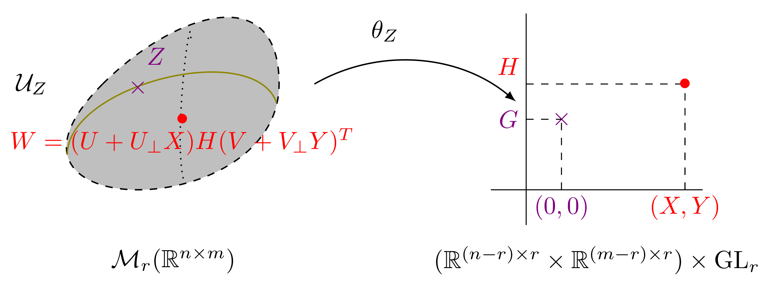
Finally, in Section 4, we provide an analytic atlas ${\mathcal{B}}_{n,m,r}={\left\{({\mathcal{U}}_Z,{\theta }_Z)\right\}}_{Z\in {\mathcal{M}}_r\left({\mathbb{R}}^{n\times m}\right)}$ for the set ${\mathcal{M}}_r\left({\mathbb{R}}^{n\times m}\right)$ of matrices $Z=UG{V}^T$ with rank $r<min\{n,m\}$, with local chart

$${\theta }_Z:{\mathcal{U}}_Z\to {\mathbb{R}}^{(n-r)\times r}\times {\mathbb{R}}^{(m-r)\times r}\times {\mathrm{GL}}_r,{\theta }_Z^{-1}(X,Y,H)=(U+U_{\perp }X)H(V+V_{\perp }Y),$$

and we prove that ${\mathcal{M}}_r\left({\mathbb{R}}^{n\times m}\right)$ is an analytic principal bundle with base ${\mathbb{G}}_r\left({\mathbb{R}}^n\right)\times {\mathbb{G}}_r\left({\mathbb{R}}^m\right)$ and typical fibre ${\mathrm{GL}}_r$. Then, we prove that ${\mathcal{M}}_r\left({\mathbb{R}}^{n\times m}\right)$ is an embedded submanifold of $({\mathbb{R}}^{n\times m},{\tau }_{{\mathbb{R}}^{n\times m}}^{*})$ and that each of the neighbourhoods ${\mathcal{U}}_Z$ have the structure of a Lie group.

2. The Grassmann Manifold ${\mathbb{G}}_{\mathit{r}}\left({\mathbb{R}}^{\mathit{k}}\right)$

In this section, we present a geometric description of the Grassmann manifold ${\mathbb{G}}_r\left({\mathbb{R}}^k\right)$ of all subspaces of dimension r in ${\mathbb{R}}^k$, $0<r<k$,

$${\mathbb{G}}_r\left({\mathbb{R}}^k\right)=\{\mathcal{V}\subset {\mathbb{R}}^k:\mathcal{V}\mathrm{is}\mathrm{a}\mathrm{linear}\mathrm{subspace}\mathrm{with}dim\left(\mathcal{V}\right)=r\},$$

with an explicit description of local charts. We first introduce the surjective map

$${\mathrm{col}}_{k,r}:{\mathcal{M}}_r\left({\mathbb{R}}^{k\times r}\right)⟶{\mathbb{G}}_r\left({\mathbb{R}}^k\right),Z\mapsto {\mathrm{col}}_{k,r}\left(Z\right),$$

where ${\mathrm{col}}_{k,r}\left(Z\right)$ is the column space of the matrix Z, which is the subspace spanned by the column vectors of $Z.$ Given $\mathcal{V}\in {\mathbb{G}}_r\left({\mathbb{R}}^k\right),$ there are infinitely many matrices Z such that ${\mathrm{col}}_{k,r}\left(Z\right)=\mathcal{V}$. Given a matrix $Z\in {\mathcal{M}}_r\left({\mathbb{R}}^{k\times r}\right)$, the set of matrices in ${\mathcal{M}}_r\left({\mathbb{R}}^{k\times r}\right)$ with the same column space as Z is

$$Z{\mathrm{GL}}_r:=\{ZG:G\in {\mathrm{GL}}_r\}.$$

2.1. An Atlas for ${\mathbb{G}}_r\left({\mathbb{R}}^k\right)$

For a given matrix Z in ${\mathcal{M}}_r\left({\mathbb{R}}^{k\times r}\right)$, we let $Z_{\perp }\in {\mathcal{M}}_{k-r}\left({\mathbb{R}}^{k\times (k-r)}\right)$ be a matrix such that $Z^T{Z}_{\perp }=0$, and we introduce an affine cross section

$$\begin{array}{c}\hfill {\mathcal{S}}_Z:=\{W\in {\mathcal{M}}_r\left({\mathbb{R}}^{k\times r}\right):Z^{T}W=Z^{T}Z\},\end{array}$$

(3)

which has the following equivalent characterization.

Lemma 1.

The affine cross section ${\mathcal{S}}_Z$ is characterized by

$$\begin{array}{c}\hfill {\mathcal{S}}_Z=\{Z+Z_{\perp }X:X\in {\mathbb{R}}^{(k-r)\times r}\},\end{array}$$

(4)

and the map

$${\eta }_Z:{\mathbb{R}}^{(k-r)\times r}⟶{\mathcal{S}}_Z,X\mapsto Z+Z_{\perp }X$$

is bijective.

Proof. 

We first observe that $Z^T(Z+Z_{\perp }{X}_Z)=Z^{T}Z$ for all $X\in {\mathbb{R}}^{(k-r)\times r}$, which implies that $\{Z+Z_{\perp }X:X\in {\mathbb{R}}^{(k-r)\times r}\}\subset {\mathcal{S}}_Z.$ For the other inclusion, we observe that if $W\in {\mathcal{S}}_Z$, then $Z^{T}W=Z^{T}Z$ and hence $W-Z\in {\mathrm{col}}_{k,r}{\left(Z\right)}^{\perp }$, the orthogonal subspace to ${\mathrm{col}}_{k,r}\left(Z\right)$ in ${\mathbb{R}}^k$. Since ${\mathrm{col}}_{k,r}{\left(Z\right)}^{\perp }={\mathrm{col}}_{k,k-r}\left(Z_{\perp }\right),$ there exists $X\in {\mathbb{R}}^{(k-r)\times r}$ such that $W-Z=Z_{\perp }X.$ Proving that ${\eta }_Z$ is bijective is straightforward. □

Proposition 1.

For each $W\in {\mathcal{M}}_r\left({\mathbb{R}}^{k\times r}\right)$ such that $det\left(Z^{T}W\right)\ne 0$, there exists a unique $G_W\in {\mathrm{GL}}_r$ such that

$$W{\mathrm{GL}}_r\cap {\mathcal{S}}_Z=\left\{W{G}_W^{-1}\right\}$$

holds, which means that the set of matrices with the same column space as W intersects ${\mathcal{S}}_Z$ at the single point $W{G}_W^{-1}.$ Furthermore, $G_W=i{d}_r$ if and only if $W\in {\mathcal{S}}_Z.$

Proof. 

By Lemma 1, a matrix $A\in W{\mathrm{GL}}_r\cap {\mathcal{S}}_Z$ is such that $A=W{G}_W^{-1}=Z+Z_{\perp }X$ for a certain $G_W\in {\mathrm{GL}}_r$ and a certain $X\in {\mathbb{R}}^{(k-r)\times r}$. Then $Z^{T}W{G}_W^{-1}=Z^{T}Z$ and $G_W$ is uniquely defined by $G_W={\left(Z^{T}Z\right)}^{-1}\left(Z^{T}W\right),$ which proves that $W{\mathrm{GL}}_r\cap {\mathcal{S}}_Z$ is the singleton $\left\{W{G}_W^{-1}\right\},$ and $G_W=i{d}_r$ if and only if $W\in {\mathcal{S}}_Z.$ □

Corollary 1.

For each $Z\in {\mathcal{M}}_r\left({\mathbb{R}}^{k\times r}\right)$, the map ${\mathrm{col}}_{k,r}:{\mathcal{S}}_Z⟶{\mathbb{G}}_r\left({\mathbb{R}}^k\right)$ is injective.

Proof. 

Let us assume the existence of $W,\tilde{W}\in {\mathcal{S}}_Z$ such that ${\mathrm{col}}_{k,r}\left(W\right)={\mathrm{col}}_{k,r}\left(\tilde{W}\right).$ Then $W=\tilde{W}$ by Proposition 1. □

Lemma 1 and Corollary 1 allow us to construct a system of local charts for ${\mathbb{G}}_r\left({\mathbb{R}}^k\right)$ by defining for each $Z\in {\mathcal{M}}_r\left({\mathbb{R}}^{k\times r}\right)$ a neighbourhood of ${\mathrm{col}}_{k,r}\left(Z\right)$ by

$${\mathfrak{U}}_Z:={\mathrm{col}}_{k,r}\left({\mathcal{S}}_Z\right)=\{{\mathrm{col}}_{k,r}\left(W\right):W\in {\mathcal{S}}_Z\}$$

together with the bijective map

$${\phi }_Z:={({\mathrm{col}}_{k,r}\circ {\eta }_Z)}^{-1}:{\mathfrak{U}}_Z\to {\mathbb{R}}^{(k-r)\times r}$$

such that

$${\phi }_Z^{-1}\left(X\right)={\mathrm{col}}_{k,r}(Z+Z_{\perp }X)$$

for $X\in {\mathbb{R}}^{(k-r)\times r}$. We denote by $Z^{+}$ the Moore–Penrose pseudo-inverse of the full rank matrix $Z\in {\mathcal{M}}_r\left({\mathbb{R}}^{r\times k}\right)$, defined by

$$Z^{+}:={\left(Z^{T}Z\right)}^{-1}{Z}^T\in {\mathcal{M}}_r\left({\mathbb{R}}^{r\times k}\right).$$

It satisfies $Z^{+}Z=i{d}_r$ and $Z^{+}{Z}_{\perp }=0$. Moreover, $Z{Z}^{+}\in {\mathbb{R}}^{k\times k}$ is the projection onto ${\mathrm{col}}_{k,r}\left(Z\right)$ parallel to ${\mathrm{col}}_{k,r}{\left(Z\right)}^{\perp }$. Finally, we have the following result.

Theorem 1.

The collection ${\mathcal{A}}_{k,r}:=\{({\mathfrak{U}}_Z,{\phi }_Z):Z\in {\mathcal{M}}_r\left({\mathbb{R}}^{k\times r}\right)\}$ is an analytic atlas for ${\mathbb{G}}_r\left({\mathbb{R}}^k\right)$ and hence $({\mathbb{G}}_r\left({\mathbb{R}}^k\right),{\mathcal{A}}_{k,r})$ is an analytic $r(k-r)$-dimensional manifold modelled on ${\mathbb{R}}^{(k-r)\times r}$.

Proof. 

Clearly ${\left\{{\mathfrak{U}}_Z\right\}}_{Z\in {\mathcal{M}}_r\left({\mathbb{R}}^{k\times r}\right)}$ is a covering of ${\mathbb{G}}_r\left({\mathbb{R}}^k\right).$ Now let Z and $\tilde{Z}$ be such that ${\mathfrak{U}}_Z\cap {\mathfrak{U}}_{\tilde{Z}}\ne \varnothing$. Let $\mathcal{V}\in {\mathfrak{U}}_Z$ such that $\mathcal{V}={\phi }_Z^{-1}\left(X\right)={\mathrm{col}}_{k,r}(Z+Z_{\perp }X)$, with $X\in {\mathbb{R}}^{k\times (k-r)}$. We can write $Z+Z_{\perp }X=(\tilde{Z}+{\tilde{Z}}_{\perp }\tilde{X})G$ with $G={\tilde{Z}}^{+}(Z+Z_{\perp }X)$ and $\tilde{X}={\tilde{Z}}_{\perp }^{+}(Z+Z_{\perp }X)G^{-1}$. Therefore, $\mathcal{V}={\mathrm{col}}_{k,r}\left((\tilde{Z}+{\tilde{Z}}_{\perp }\tilde{X})G\right)={\mathrm{col}}_{k,r}(\tilde{Z}+{\tilde{Z}}_{\perp }\tilde{X})={\phi }_{\tilde{Z}}^{-1}\left(\tilde{X}\right)\in {\mathfrak{U}}_{\tilde{Z}}$, which implies that ${\mathfrak{U}}_Z={\mathfrak{U}}_Z\cap {\mathfrak{U}}_{\tilde{Z}}$. Therefore, ${\phi }_Z({\mathfrak{U}}_Z\cap {\mathfrak{U}}_{\tilde{Z}})={\phi }_Z\left({\mathfrak{U}}_Z\right)={\mathbb{R}}^{k\times (n-k)}$ is an open set. In the same way, we show that ${\mathfrak{U}}_{\tilde{Z}}={\mathfrak{U}}_Z\cap {\mathfrak{U}}_{\tilde{Z}}$ and ${\phi }_{\tilde{Z}}\left({\mathfrak{U}}_Z\right)={\mathbb{R}}^{k\times (n-k)}$ is an open set. Finally, the map ${\phi }_{\tilde{Z}}\circ {\phi }_Z^{-1}$ from ${\mathbb{R}}^{(k-r)\times r}$ to ${\mathbb{R}}^{(k-r)\times r}$ is given by ${\phi }_{\tilde{Z}}\circ {\phi }_Z^{-1}\left(X\right)={\tilde{Z}}_{\perp }^{+}(Z+Z_{\perp }X)G^{-1}$, with $G={\tilde{Z}}^{+}(Z+Z_{\perp }{X}_Z)$, which is clearly an analytic map. □

Remark 1.

A possible choice for $Z_{\perp }$ satisfying $Z_{\perp }^{T}Z=0$ is $Z_{\perp }=(i{d}_k-Z{Z}^{+})B_{\perp }$ where $B_{\perp }\in {\mathcal{M}}_{k-r}\left({\mathbb{R}}^{k\times (k-r)}\right)$ is such that its column space is a complement of the column space of Z. In practice, we can determine a set of r linear independent rows of Z (see, e.g., [25,26]), with indices I, and then choose $B_{\perp }$ such that ${\left(B_{\perp }\right)}_{i,j}={\delta }_{i,j}$ if $i\notin I$ and 0 if $i\in I$, for $1\le i\le k$, $1\le j\le k-r$. For a given $X\in {\mathbb{R}}^{(k-r)\times r}$, the computation of $Z_{\perp }X$ does not require $Z_{\perp }$ and has a complexity $O\left(r^{2}k\right)$.

2.2. Lie Group Structure of Neighbourhoods ${\mathfrak{U}}_Z$

Here we prove that each neighbourhood ${\mathfrak{U}}_Z$ of ${\mathbb{G}}_r\left({\mathbb{R}}^k\right)$ is a Lie group. For that, we first note that a neighbourhood ${\mathfrak{U}}_Z$ of ${\mathbb{G}}_r\left({\mathbb{R}}^k\right)$ can be identified with the set ${\mathcal{S}}_Z$ through the application ${\mathrm{col}}_{k,r}:{\mathcal{S}}_Z\to {\mathfrak{U}}_Z$. The next step is to identify ${\mathcal{S}}_Z$ with a closed Lie subgroup of ${\mathrm{GL}}_k,$ denoted by ${\mathcal{G}}_Z,$ with associated Lie algebra ${\mathfrak{g}}_Z$ isomorphic to ${\mathbb{R}}^{r\times (k-r)}$, and such that the exponential map $exp:{\mathfrak{g}}_Z⟶{\mathcal{G}}_Z$ is a diffeomorphism. (We recall that the matrix exponential $exp:{\mathbb{R}}^{k\times k}\to {\mathrm{GL}}_k$ is defined by $exp\left(A\right)={\sum }_{n=0}^{\infty }\frac{A^n}{n!}.$) To this end, for a given $Z\in {\mathcal{M}}_r\left({\mathbb{R}}^{k\times r}\right)$, we introduce the vector space

$$\begin{array}{c}\hfill {\mathfrak{g}}_Z:=\{Z_{\perp }X{Z}^{+}:X\in {\mathbb{R}}^{(k-r)\times r}\}\subset {\mathbb{R}}^{k\times k}.\end{array}$$

(5)

The following proposition proves that ${\mathfrak{g}}_Z$ is a commutative subalgebra of ${\mathbb{R}}^{k\times k}.$

Proposition 2.

For all $X,\tilde{X}\in {\mathbb{R}}^{(k-r)\times r}$,

$$\left(Z_{\perp }X{Z}^{+}\right)\left(Z_{\perp }\tilde{X}{Z}^{+}\right)=0$$

holds, and ${\mathfrak{g}}_Z$ is a commutative subalgebra of ${\mathbb{R}}^{k\times k}.$ Moreover,

$$\begin{array}{c}\hfill exp\left(Z_{\perp }X{Z}^{+}\right)=i{d}_k+Z_{\perp }X{Z}^{+},\end{array}$$

(6)

$$\begin{array}{c}\hfill exp\left(Z_{\perp }X{Z}^{+}\right)Z=Z+Z_{\perp }X,\end{array}$$

(7)

and

$$\begin{array}{c}\hfill exp\left(Z_{\perp }X{Z}^{+}\right)Z_{\perp }=Z_{\perp }\end{array}$$

(8)

hold for all $X\in {\mathbb{R}}^{(k-r)\times r}.$

Proof. 

Since $\left(Z_{\perp }X{Z}^{+}\right)\left(Z_{\perp }\tilde{X}{Z}^{+}\right)=0$ holds for all $X,\tilde{X}\in {\mathbb{R}}^{(k-r)\times r},$ the vector space ${\mathfrak{g}}_Z$ is a closed subalgebra of the matrix unitary algebra ${\mathbb{R}}^{k\times k}.$ As a consequence, ${\left(Z_{\perp }X{Z}^{+}\right)}^p=0$ holds for all $X\in {\mathbb{R}}^{(k-r)\times r}$ and all $p\ge 2$, which proves (6). We directly deduce (7) using $Z{Z}^{+}=i{d}_r$ and (8) using $Z^{+}{Z}_{\perp }=0$. □

From Proposition 2 and the definition of ${\mathcal{S}}_Z$, we obtain the following results.

Corollary 2.

The affine cross section ${\mathcal{S}}_Z$ satisfies

$$\begin{array}{c}\hfill {\mathcal{S}}_Z=\{exp\left(Z_{\perp }X{Z}^{+}\right)Z:X\in {\mathbb{R}}^{(k-r)\times r}\},\end{array}$$

(9)

and

$$\begin{array}{c}\hfill [exp\left(Z_{\perp }X{Z}^{+}\right)Z|Z_{\perp }]\in {\mathrm{GL}}_k\end{array}$$

(10)

for all $X\in {\mathbb{R}}^{(k-r)\times r}$, where the brackets $\left[·|·\right]$ are used for matrix concatenation.

Proof. 

From Proposition 2 and (4), we obtain (9) and we can write

$$[exp\left(Z_{\perp }X{Z}^{+}\right)Z|Z_{\perp }]=[exp\left(Z_{\perp }X{Z}^{+}\right)Z|exp\left(Z_{\perp }X{Z}^{+}\right)Z_{\perp }]=exp\left(Z_{\perp }X{Z}^{+}\right)\left[Z\right|Z_{\perp }].$$

Since $exp\left(Z_{\perp }X{Z}^{+}\right),\left[Z\right|Z_{\perp }]\in {\mathrm{GL}}_k$, (10) follows. □

Now we need to introduce the following definition and proposition (see ([27] p. 80)).

Definition 1.

Let $(\mathbb{K},+,·)$ be a ring and let $(\mathbb{K},+)$ be its additive group. A subset $\mathbb{I}\subset \mathbb{K}$ is called a two-sided ideal (or simply an ideal) of $\mathbb{K}$ if it is an additive subgroup of $\mathbb{K}$ such that $\mathbb{I}·\mathbb{K}:=\{r·x:r\in \mathbb{I}\mathrm{and}x\in \mathbb{K}\}\subset \mathbb{I}$ and $\mathbb{K}·\mathbb{I}:=\{x·r:r\in \mathbb{I}\mathrm{and}x\in \mathbb{K}\}\subset \mathbb{I}.$

Proposition 3.

If $\mathfrak{g}\subset \mathfrak{h}$ is a two-sided ideal of the Lie algebra $\mathfrak{h}$ of a group $\mathcal{H}$, then the subgroup $\mathcal{G}\subset \mathcal{H}$ generated by $exp\left(\mathfrak{g}\right)=\{exp(G):G\in \mathfrak{g}\}$ is normal and closed, with Lie algebra $\mathfrak{h}.$

From the above proposition, we deduce the following result.

Lemma 2.

Let $Z\in {\mathcal{M}}_r\left({\mathbb{R}}^{k\times r}\right)$ and $Z_{\perp }\in {\mathcal{M}}_{k-r}\left({\mathbb{R}}^{k\times (k-r)}\right)$ be such that $Z^T{Z}_{\perp }=0.$ Then ${\mathfrak{g}}_Z\subset {\mathbb{R}}^{k\times k}$ is a two-sided ideal of the Lie algebra ${\mathbb{R}}^{k\times k}$ and hence

$$\begin{array}{c}\hfill {\mathcal{G}}_Z:=\{exp\left(Z_{\perp }X{Z}^{+}\right):X\in {\mathbb{R}}^{(k-r)\times r}\}\end{array}$$

(11)

is a closed Lie group with Lie algebra ${\mathfrak{g}}_Z.$ Furthermore, the map $exp:{\mathfrak{g}}_Z⟶{\mathcal{G}}_Z$ is bijective.

Proof. 

Consider $Z_{\perp }X{Z}^{+}\in {\mathfrak{g}}_Z$ and $A\in {\mathbb{R}}^{k\times k}$. Noting that $Z^{+}Z=i{d}_r$ and ${\left(Z_{\perp }\right)}^{+}{Z}_{\perp }=i{d}_{k-r}$, we have that

$$\left(Z_{\perp }X{Z}^{+}\right)A=Z_{\perp }\left(X{Z}^{+}AZ\right)Z^{+},$$

which proves that ${\mathfrak{g}}_Z·{\mathbb{R}}^{k\times k}\subset {\mathfrak{g}}_Z.$ Similarly, we have that

$$A\left(Z_{\perp }X{Z}^{+}\right)=Z_{\perp }\left({\left(Z_{\perp }\right)}^{+}A{Z}_{\perp }X\right)Z^{+},$$

which proves that ${\mathbb{R}}^{k\times k}·{\mathfrak{g}}_Z\subset {\mathfrak{g}}_Z.$ This proves that ${\mathfrak{g}}_Z$ is a two-sided ideal. The map exp is clearly surjective. To prove that it is injective, we assume $exp\left(Z_{\perp }X{Z}^{+}\right)=exp\left(Z_{\perp }\tilde{X}{Z}^{+}\right)$ for $X,\tilde{X}\in {\mathbb{R}}^{(k-r)\times r}$. Then, from (6), we obtain $Z+Z_{\perp }X=Z+Z_{\perp }\tilde{X}$ and hence $X=\tilde{X}$, i.e., $Z_{\perp }X{Z}^{+}=Z_{\perp }\tilde{X}{Z}^{+}$ in ${\mathfrak{g}}_Z.$ □

Finally, we can prove the following result.

Theorem 2.

The set ${\mathcal{S}}_Z$ together with the group operation ${\times }_Z$ defined by

$$\begin{array}{c}\hfill exp\left(Z_{\perp }X{Z}^{+}\right)Z{\times }_{Z}exp\left(Z_{\perp }\tilde{X}{Z}^{+}\right)Z=exp\left(Z_{\perp }(X+\tilde{X})Z^{+}\right)Z\end{array}$$

(12)

for $X,\tilde{X}\in {\mathbb{R}}^{(k-r)\times r}$ is a Lie group.

Proof. 

To prove that it is a Lie group, we simply note that the multiplication and inversion maps

$$\mu :{\mathcal{S}}_Z\times {\mathcal{S}}_Z⟶{\mathcal{S}}_Z,(W,\tilde{W})\mapsto exp\left(Z_{\perp }(Z_{\perp }^{+}(W-Z)+Z_{\perp }^{+}(\tilde{W}-Z))Z^{+}\right)Z$$

and

$$\delta :{\mathcal{S}}_Z⟶{\mathcal{S}}_Z,W\mapsto exp(-Z_{\perp }{Z}_{\perp }^{+}(W-Z)Z^{+})Z$$

are analytic. □

It follows that ${\mathfrak{U}}_Z$ can be identified with a Lie group through the map ${\phi }_Z$.

Theorem 3.

Each neighbourhood ${\mathfrak{U}}_Z$ of ${\mathbb{G}}_r\left({\mathbb{R}}^k\right)$ together with the group operation ${\circ }_Z$ defined by

$$\mathcal{V}{\circ }_Z{\mathcal{V}}^{\prime }={\phi }_Z^{-1}({\phi }_Z\left(\mathcal{V}\right)+{\phi }_Z\left({\mathcal{V}}^{\prime }\right))$$

for $\mathcal{V},{\mathcal{V}}^{\prime }\in {\mathfrak{U}}_Z$, is a Lie group, and the map ${\gamma }_Z:{\mathfrak{U}}_Z⟶{\mathcal{G}}_Z$ given by

$${\gamma }_Z\left(\mathcal{U}\right)=exp\left(Z_{\perp }{\phi }_Z\left(\mathcal{U}\right)Z^{+}\right)$$

is a Lie group isomorphism.

3. The Non-Compact Stiefel Principal Bundle ${\mathcal{M}}_r\left({\mathbb{R}}^{k\times r}\right)$

In this section, we give a new geometric description of the set ${\mathcal{M}}_r\left({\mathbb{R}}^{k\times r}\right)$ of matrices with full rank $r<k$, which is based on the geometric description of the Grassmann manifold given in Section 2.

3.1. Principal Bundle Structure of ${\mathcal{M}}_r\left({\mathbb{R}}^{k\times r}\right)$

For $Z\in {\mathcal{M}}_r\left({\mathbb{R}}^{k\times r}\right)$, we define a neighbourhood of Z as

$$\begin{array}{c}\hfill {\mathcal{V}}_Z:=\{W\in {\mathcal{M}}_r\left({\mathbb{R}}^{k\times r}\right):det\left(Z^{T}W\right)\ne 0\}\supset {\mathcal{S}}_Z.\end{array}$$

(13)

From Proposition 1, we know that for a given matrix $W\in {\mathcal{V}}_Z$, there exists a unique pair of matrices $(X,G)\in {\mathbb{R}}^{(k-r)\times r}\times {\mathrm{GL}}_r$ such that $W=(Z+Z_{\perp }X)G.$ Therefore,

$${\mathcal{V}}_Z=\{(Z+Z_{\perp }X)G:X\in {\mathbb{R}}^{(k-r)\times r},G\in {\mathrm{GL}}_r\}.$$

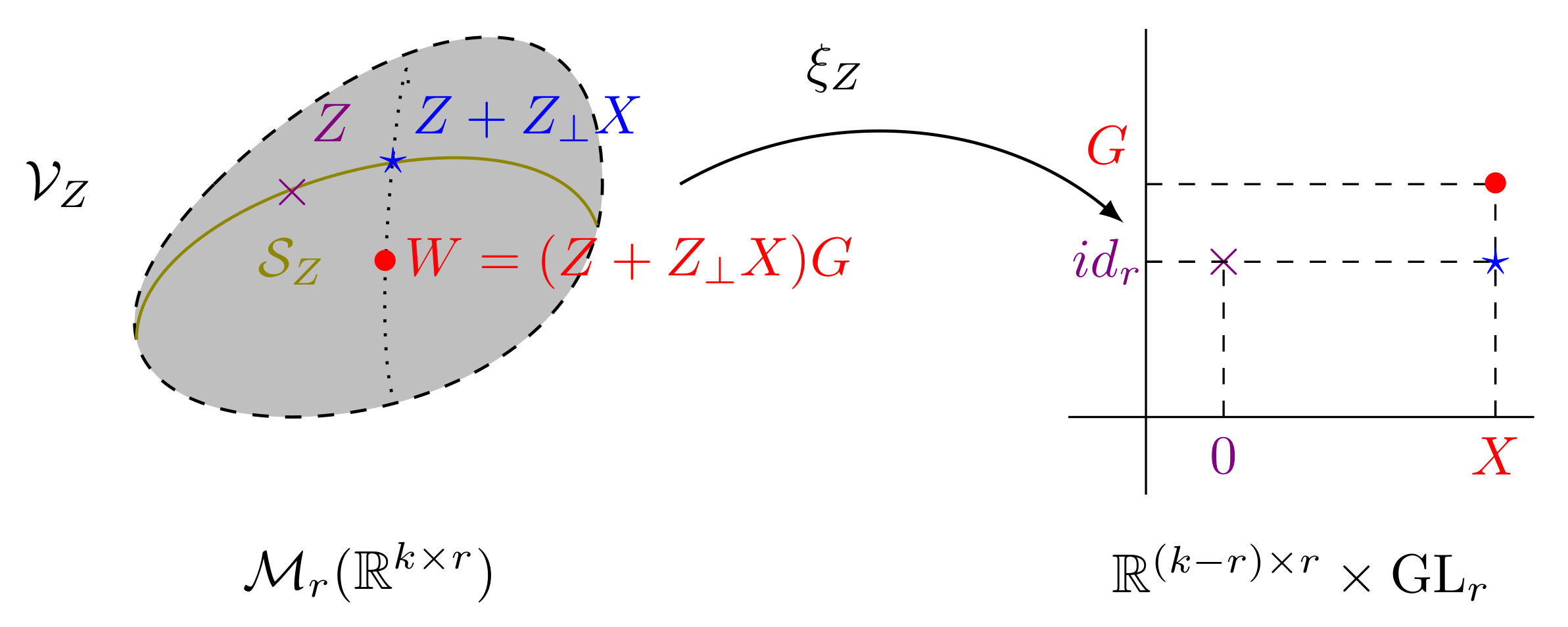
It allows us to introduce a parametrisation ${\xi }_Z^{-1}$ (see Figure 1) defined through the bijection

$$\begin{array}{c}\hfill {\xi }_Z:{\mathcal{V}}_Z⟶{\mathbb{R}}^{(k-r)\times r}\times {\mathrm{GL}}_r,\end{array}$$

(14)

such that

$${\xi }_Z^{-1}(X,G)=(Z+Z_{\perp }X)G$$

for $(X,G)\in {\mathbb{R}}^{(k-r)\times r}\times {\mathrm{GL}}_r$ and

$$\begin{array}{c}\hfill {\xi }_Z\left(W\right)=(Z_{\perp }^{+}W{\left(Z^{+}W\right)}^{-1},Z^{+}W)\end{array}$$

for $W\in {\mathcal{V}}_Z$. In particular,

$${\xi }_Z^{-1}(0,i{d}_r)=Z.$$

Theorem 4.

The collection ${\mathcal{B}}_{k,r}:=\{({\mathcal{V}}_Z,{\xi }_Z):Z\in {\mathcal{M}}_r\left({\mathbb{R}}^{k\times r}\right)\}$ is an analytic atlas for ${\mathcal{M}}_r\left({\mathbb{R}}^{k\times r}\right)$, and hence $({\mathcal{M}}_r\left({\mathbb{R}}^{k\times r}\right),{\mathcal{B}}_{k,r})$ is an analytic $kr$-dimensional manifold modelled on ${\mathbb{R}}^{(k-r)\times r}\times {\mathbb{R}}^{r\times r}.$

Proof. 

${\left\{{\mathcal{V}}_Z\right\}}_{Z\in {\mathcal{M}}_r\left({\mathbb{R}}^{k\times r}\right)}$ is clearly a covering of ${\mathcal{M}}_r\left({\mathbb{R}}^{k\times r}\right)$. Moreover, since ${\xi }_Z$ is bijective from ${\mathcal{V}}_Z$ to ${\mathbb{R}}^{(k-r)\times r}\times {\mathrm{GL}}_r$ we claim that if ${\mathcal{V}}_Z\cap {\mathcal{V}}_{\tilde{Z}}\ne \varnothing$ for $Z,\tilde{Z}\in {\mathcal{M}}_r\left({\mathbb{R}}^{k\times r}\right),$ then the following statements hold:

(i)

${\xi }_Z({\mathcal{V}}_Z\cap {\mathcal{V}}_{\tilde{Z}})$ and ${\xi }_{\tilde{Z}}({\mathcal{V}}_Z\cap {\mathcal{V}}_{\tilde{Z}})$ are open sets in ${\mathbb{R}}^{(k-r)\times r}\times {\mathrm{GL}}_r$ and

(ii)

the map ${\xi }_{\tilde{Z}}\circ {\xi }_Z^{-1}$ is analytic from ${\xi }_Z({\mathcal{V}}_Z\cap {\mathcal{V}}_{\tilde{Z}})\subset {\mathbb{R}}^{(k-r)\times r}\times {\mathrm{GL}}_r$ to ${\xi }_{\tilde{Z}}({\mathcal{V}}_Z\cap {\mathcal{V}}_{\tilde{Z}})\subset {\mathbb{R}}^{(k-r)\times r}\times {\mathrm{GL}}_r$.

In this proof, we equip ${\mathbb{R}}^{k\times r}$ with the topology ${\tau }_{{\mathbb{R}}^{k\times r}}$ induced by matrix norms. For any $Z\in {\mathcal{M}}_r\left({\mathbb{R}}^{k\times r}\right)$, ${\mathcal{V}}_Z=\{W\in {\mathbb{R}}^{k\times r}:det\left(Z^{T}W\right)\ne 0\}$ is the inverse image of the open set $\mathbb{R}\setminus \left\{0\right\}$ by the continuous map $W\mapsto det\left(Z^{T}W\right)$ from ${\mathbb{R}}^{k\times r}$ to $\mathbb{R}$, and therefore, ${\mathcal{V}}_Z$ is an open set of ${\mathbb{R}}^{k\times r}$. Since ${\mathcal{V}}_Z$ and ${\mathcal{V}}_{\tilde{Z}}$ are open sets in ${\mathbb{R}}^{k\times r}$, ${\mathcal{V}}_Z\cap {\mathcal{V}}_{\tilde{Z}}$ is also an open set in ${\mathbb{R}}^{k\times r}$ and since ${\xi }_Z^{-1}$ is a continuous map from ${\mathbb{R}}^{(k-r)\times r}\times {\mathrm{GL}}_r$ to ${\mathbb{R}}^{k\times r}$, the set ${\xi }_Z({\mathcal{V}}_Z\cap {\mathcal{V}}_{\tilde{Z}})$, as the inverse image of an open set by a continuous map, is an open set in ${\mathbb{R}}^{(k-r)\times r}\times {\mathrm{GL}}_r$. Similarly, ${\xi }_{\tilde{Z}}({\mathcal{V}}_Z\cap {\mathcal{V}}_{\tilde{Z}})$ is an open set. Now let $(X,G)\in {\mathbb{R}}^{(k-r)\times r}\times {\mathrm{GL}}_r$ such that ${\xi }_Z^{-1}(X,G)\in {\mathcal{V}}_Z\cap {\mathcal{V}}_{\tilde{Z}}$. From the expressions of ${\xi }_Z^{-1}$ and ${\xi }_{\tilde{Z}}$, the map ${\xi }_{\tilde{Z}}\circ {\xi }_Z^{-1}$ is defined by

$$\begin{array}{cc}\hfill {\xi }_{\tilde{Z}}\circ {\xi }_Z^{-1}(X,G)& =({\tilde{Z}}_{\perp }^{+}{\xi }_Z^{-1}(X,G){\left({\tilde{Z}}^{+}{\xi }_Z^{-1}(X,G)\right)}^{-1},{\tilde{Z}}^{+}{\xi }_Z^{-1}(X,G)),\hfill \end{array}$$

with ${\xi }_Z^{-1}(X,G)=(Z+Z_{\perp }X)G$, which is clearly an analytic map. □

Before stating the next result, we recall the definition of a morphism between manifolds and of a fibre bundle. We introduce notions of $C^p$ maps and $C^p$ manifolds, with $p\in \mathbb{N}\cup \{\infty \}$ or $p=\omega$. In the latter case, $C^{\omega }$ means analytic.

Definition 2.

Let $(\mathbb{M},\mathcal{A})$ and $(\mathbb{N},\mathcal{B})$ be two $C^p$ manifolds. Let $F:\mathbb{M}\to \mathbb{N}$ be a map. We say that F is a $C^p$ morphism between $(\mathbb{M},\mathcal{A})$ and $(\mathbb{N},\mathcal{B})$ if given $m\in \mathbb{M}$, there exists a chart $(U,\phi )\in \mathcal{A}$ such that $m\in U$ and a chart $(W,\psi )\in \mathcal{B}$ such that $F\left(m\right)\in W$ where $F\left(U\right)\subset W,$ and the map

$$\psi \circ F\circ {\phi }^{-1}:\phi \left(U\right)\to \psi \left(W\right)$$

is a map of class $C^p$. If it is a $C^p$ diffeomorphism, then we say that F is a$C^p$ diffeomorphism between manifolds. We say that $\psi \circ F\circ {\phi }^{-1}$ is a representation of F using a system of local coordinates given by the charts $(U,\phi )$ and $(W,\psi ).$

Definition 3.

Let $\mathbb{B}$ be a $C^p$ manifold with atlas $\mathcal{A}=\{(U_b,{\phi }_b):b\in \mathbb{B}\}$, and let $\mathbb{F}$ be a manifold. A $C^p$ fibre bundle $\mathbb{E}$ with base $\mathbb{B}$ and typical fibre $\mathbb{F}$ is a $C^p$ manifold which is locally a product manifold; that is, there exists a surjective morphism $\pi :\mathbb{E}⟶\mathbb{B}$ such that for each $b\in \mathbb{B}$ there is a $C^p$ diffeomorphism between manifolds

$${\chi }_b:{\pi }^{-1}\left(U_b\right)⟶U_b\times \mathbb{F},$$

such that$p_b\circ {\chi }_b=\pi$where$p_b:U_b\times \mathbb{F}⟶U_b$is the projection. For each$b\in \mathbb{B},$${\pi }^{-1}\left(b\right)={\mathbb{E}}_b$is called the fibre over$b.$The$C^p$diffeomorphisms${\chi }_b$are called fibre bundle charts. If$p=0,$$\mathbb{E},\mathbb{B}$and$\mathbb{F}$are only required to be topological spaces and$\{U_b:b\in \mathbb{B}\}$an open covering of$\mathbb{B}.$In the case where$\mathbb{F}$is a Lie group, we say that$\mathbb{E}$is a$C^p$ principal bundle, and if $\mathbb{F}$ is a vector space, we say that it is a $C^p$ vector bundle.

Theorem 5.

The set ${\mathcal{M}}_r\left({\mathbb{R}}^{k\times r}\right)$ is an analytic principal bundle with typical fibre ${\mathrm{GL}}_r$ and base ${\mathbb{G}}_r\left({\mathbb{R}}^k\right)$, with a surjective morphism between ${\mathcal{M}}_r\left({\mathbb{R}}^{k\times r}\right)$ and ${\mathbb{G}}_r\left({\mathbb{R}}^k\right)$ given by the map ${\mathrm{col}}_{k,r}$.

Proof. 

To show that it is an analytic principal bundle, we first observe that

$${\mathrm{col}}_{k,r}:({\mathcal{M}}_r\left({\mathbb{R}}^{k\times r}\right),{\mathcal{B}}_{k,r})⟶({\mathbb{G}}_r\left({\mathbb{R}}^k\right),{\mathcal{A}}_{k,r})$$

is a surjective morphism. Indeed, let $Z\in {\mathcal{M}}_r\left({\mathbb{R}}^{k\times r}\right)$ and $({\mathcal{V}}_Z,{\xi }_Z)\in {\mathcal{B}}_{k,r}$ and $({\mathfrak{U}}_Z,{\phi }_Z)\in {\mathcal{A}}_{k,r}$. Noting that ${\mathrm{col}}_{k,r}\left(YG\right)={\mathrm{col}}_{k,r}\left(Y\right)$ for all $Y\in {\mathcal{S}}_Z$, we obtain that ${\mathrm{col}}_{k,r}\left({\mathcal{V}}_Z\right)={\mathfrak{U}}_Z$. Moreover, a representation of ${\mathrm{col}}_{k,r}$ by using a system of local coordinates given by the charts is

$$({\phi }_Z\circ {\mathrm{col}}_{k,r}\circ {\xi }_Z^{-1})(X,G)=X,$$

which is clearly an analytic map from ${\mathbb{R}}^{(k-r)\times r}\times {\mathrm{GL}}_r$ to ${\mathbb{R}}^{(k-r)\times r}$ such that ${\mathrm{col}}_{k,r}^{-1}\left({\mathfrak{U}}_Z\right)={\mathcal{V}}_Z.$ Now, a representation of the morphism

$${\chi }_Z:({\mathcal{V}}_Z,\left\{({\mathcal{V}}_Z,{\xi }_Z)\right\})⟶({\mathfrak{U}}_Z,\left\{({\mathfrak{U}}_Z,{\phi }_Z)\right\})\times ({\mathrm{GL}}_r,\left\{({\mathrm{GL}}_r,i{d}_{{\mathbb{R}}^{r\times r}})\right\}),W\mapsto ({\mathrm{col}}_{k,r}\left(W\right),G)$$

using the system of local coordinates given by the charts is

$$(({\phi }_Z\times i{d}_{{\mathbb{R}}^{r\times r}})\circ {\chi }_Z\circ {\xi }_Z^{-1}):{\mathbb{R}}^{(k-r)\times r}\times {\mathrm{GL}}_r⟶{\mathbb{R}}^{(k-r)\times r}\times {\mathrm{GL}}_r,$$

defined by

$$(({\phi }_Z\times i{d}_{{\mathbb{R}}^{r\times r}})\circ {\chi }_Z\circ {\xi }_Z^{-1})(X,G)=(X,G),$$

which is clearly an analytic diffeomorphism. To conclude, consider the projection

$$p_Z:{\mathfrak{U}}_Z\times {\mathrm{GL}}_r⟶{\mathfrak{U}}_Z,(\mathfrak{V},G)\mapsto \mathfrak{V},$$

and observe that $(p_Z\circ {\chi }_Z)\left(W\right)={\mathrm{col}}_{k,r}\left(W\right)$ holds for all $W\in {\mathcal{V}}_Z.$ □

3.2. ${\mathcal{M}}_r\left({\mathbb{R}}^{k\times r}\right)$ as a Submanifold and Its Tangent Space

Here, we prove that the non-compact Stiefel manifold ${\mathcal{M}}_r\left({\mathbb{R}}^{k\times r}\right)$ equipped with the topology given by the atlas ${\mathcal{B}}_{k,r}$ is an embedded submanifold in ${\mathbb{R}}^{k\times r}$. For that, we have to prove that the standard inclusion map

$$i:({\mathcal{M}}_r\left({\mathbb{R}}^{k\times r}\right),{\mathcal{B}}_{k,r})⟶({\mathbb{R}}^{k\times r},\left\{({\mathbb{R}}^{k\times r},i{d}_{{\mathbb{R}}^{k\times r}})\right\})$$

as a morphism is an embedding. To see this, we need to recall some definitions and results.

Definition 4.

Let $F:(\mathbb{M},\mathcal{A})\to (\mathbb{N},\mathcal{B})$ be a morphism between $C^p$ manifolds and let $m\in \mathbb{M}.$ We say that F is an immersion at mif there exists an open neighbourhood $U_m$ of m in $\mathbb{M}$ such that the restriction of F to $U_m$ induces an isomorphism from $U_m$ onto a submanifold of $\mathbb{N}.$ We say that F is an immersion if it is an immersion at each point of $\mathbb{M}.$

The next step is to recall the definition of the differential as a morphism which gives a linear map between the tangent spaces of the manifolds (in local coordinates) involved with the morphism. Let us recall that for any $m\in \mathbb{M}$, we denote by ${\mathbb{T}}_m\mathbb{M}$ the tangent space of $\mathbb{M}$ at m (in local coordinates).

Definition 5.

Let $(\mathbb{M},\mathcal{A})$ and $(\mathbb{N},\mathcal{B})$ be two $C^p$ manifolds. Let $F:(\mathbb{M},\mathcal{A})\to (\mathbb{N},\mathcal{B})$ be a morphism of class $C^p$; i.e., for any $m\in \mathbb{M}$,

$$\psi \circ F\circ {\phi }^{-1}:\phi \left(U\right)\to \psi \left(W\right)$$

is a map of class $C^p$, where $(U,\phi )\in \mathcal{A}$ is a chart in $\mathbb{M}$ containing m and $(W,\psi )\in \mathcal{B}$ is a chart in $\mathbb{N}$ containing $F\left(m\right)$. Then we define

$${\mathrm{T}}_{m}F:{\mathbb{T}}_m\left(\mathbb{M}\right)⟶{\mathbb{T}}_{F\left(m\right)}\left(\mathbb{N}\right),\upsilon \mapsto D(\psi \circ F\circ {\phi }^{-1})\left(\phi \left(m\right)\right)\left[\upsilon \right].$$

For finite dimensional manifolds we have the following criterion for immersions (see Theorem 3.5.7 in [28]).

Proposition 4.

Let $(\mathbb{M},\mathcal{A})$ and $(\mathbb{N},\mathcal{B})$ be $C^p$ manifolds. Let

$$F:(\mathbb{M},\mathcal{A})\to (\mathbb{N},\mathcal{B})$$

be a $C^p$ morphism and $m\in \mathbb{M}.$ Then F is an immersion at m if and only if ${\mathrm{T}}_{m}F$ is injective.

A concept related to an immersion between manifolds is given in the following definition.

Definition 6.

Let$(\mathbb{M},\mathcal{A})$ and $(\mathbb{N},\mathcal{B})$ be $C^p$ manifolds and let $f:(\mathbb{M},\mathcal{A})⟶(\mathbb{N},\mathcal{B})$ be a $C^p$ morphism. If f is an injective immersion, then $f\left(\mathbb{M}\right)$ is called an immersed submanifold of $\mathbb{N}$.

Finally, we give the definition of embedding.

Definition 7.

Let$(\mathbb{M},\mathcal{A})$ and $(\mathbb{N},\mathcal{B})$ be $C^p$ manifolds and let $f:(\mathbb{M},\mathcal{A})⟶(\mathbb{N},\mathcal{B})$ be a $C^p$ morphism. If f is an injective immersion, and $f:(\mathbb{M},{\tau }_{\mathcal{A}})⟶(f\left(\mathbb{M}\right),{\tau }_{\mathcal{B}}{|}_{f\left(\mathbb{M}\right)})$ is a topological homeomorphism, then we say that f is an embedding and $f\left(\mathbb{M}\right)$ is called an embedded submanifold of $\mathbb{N}$.

We first note that the representation of the inclusion map i using the system of local coordinates given by the charts $({\mathcal{V}}_Z,{\xi }_Z)\in {\mathcal{B}}_{k,r}$ in ${\mathcal{M}}_r\left({\mathbb{R}}^{k\times r}\right)$ and $({\mathbb{R}}^{k\times r},i{d}_{{\mathbb{R}}^{k\times r}})$ in ${\mathbb{R}}^{k\times r}$ is

$$(i{d}_{{\mathbb{R}}^{k\times r}}\circ i\circ {\xi }_Z^{-1})=(i\circ {\xi }_Z^{-1}):{\mathbb{R}}^{(k-r)\times r}\times {\mathrm{GL}}_r\to {\mathbb{R}}^{k\times r},(X,G)\mapsto (Z+Z_{\perp }X)G.$$

Then the tangent map $T_{Z}i$ at $Z={\xi }_Z^{-1}(0,i{d}_r)$, defined by $T_{Z}i=D(i\circ {\xi }_Z^{-1})(0,i{d}_r)$, is

$$\begin{array}{c}\hfill T_{Z}i:{\mathbb{R}}^{(k-r)\times r}\times {\mathbb{R}}^{r\times r}\to {\mathbb{R}}^{k\times r},(\dot{X},\dot{G})\mapsto Z_{\perp }\dot{X}+Z\dot{G}.\end{array}$$

Proposition 5.

The tangent map ${\mathrm{T}}_{Z}i:{\mathbb{R}}^{(k-r)\times r}\times {\mathbb{R}}^{r\times r}\to {\mathbb{R}}^{k\times r}$ at $Z\in {\mathcal{M}}_r\left({\mathbb{R}}^{k\times r}\right)$ is a linear isomorphism, with inverse ${\left({\mathrm{T}}_{Z}i\right)}^{-1}$ given by

$${\left({\mathrm{T}}_{Z}i\right)}^{-1}\left(\dot{Z}\right)=(Z_{\perp }^{+}\dot{Z},Z^{+}\dot{Z}),$$

for $\dot{Z}\in {\mathbb{R}}^{k\times r}$. Furthermore, the standard inclusion map i is an embedding from ${\mathcal{M}}_r\left({\mathbb{R}}^{k\times r}\right)$ to ${\mathbb{R}}^{k\times r}.$

Proof. 

Let us assume that ${\mathrm{T}}_{Z}i(\dot{X},\dot{G})=Z_{\perp }\dot{X}+Z\dot{G}=0.$ Multiplying this equality by $Z^{+}$ and $Z_{\perp }^{+}$ on the left, we obtain $\dot{G}=0$ and $\dot{X}=0$, respectively, which implies that ${\mathrm{T}}_{Z}i$ is injective. To prove that it is also surjective, we consider a matrix $\dot{Z}\in {\mathbb{R}}^{k\times r}$ and observe that $\dot{X}=Z_{\perp }^{+}\dot{Z}\in {\mathbb{R}}^{(k-r)\times r}$ and $\dot{G}=Z^{+}\dot{Z}\in {\mathbb{R}}^{r\times r}$ is such that ${\mathrm{T}}_{Z}i(\dot{X},\dot{G})=\dot{Z}$. Since ${\mathrm{T}}_{Z}i$ is injective, the inclusion map i is an immersion.

To prove that it is an embedding, we equip ${\mathcal{M}}_r\left({\mathbb{R}}^{k\times r}\right)$ with the topology ${\tau }_{{\mathcal{B}}_{k,r}}$ given by the atlas and we equip ${\mathbb{R}}^{k\times r}$ with the topology ${\tau }_{{\mathbb{R}}^{k\times r}}$ induced by matrix norms. We need to check that

$$i:({\mathcal{M}}_r\left({\mathbb{R}}^{k\times r}\right),{\tau }_{{\mathcal{B}}_{k,r}})⟶({\mathcal{M}}_r\left({\mathbb{R}}^{k\times r}\right),{\tau }_{{\mathbb{R}}^{k\times r}}{|}_{{\mathcal{M}}_r\left({\mathbb{R}}^{k\times r}\right)})$$

is a topological homeomorphism. Since the topology in $({\mathcal{M}}_r\left({\mathbb{R}}^{k\times r}\right),{\tau }_{{\mathcal{B}}_{k,r}})$ has the property that each local chart ${\xi }_Z$ is indeed a homeomorphism from ${\mathcal{V}}_Z$ in ${\mathcal{M}}_r\left({\mathbb{R}}^{k\times r}\right)$ to ${\xi }_Z\left({\mathcal{V}}_Z\right)={\mathbb{R}}^{(k-r)\times r}\times {\mathrm{GL}}_r$ (see Section 1.1), we only need to show that the bijection $(i\circ {\xi }_Z^{-1}):{\mathbb{R}}^{(k-r)\times r}\times {\mathrm{GL}}_r\to {\mathcal{V}}_Z\subset {\mathbb{R}}^{k\times r}$ given by

$$(i\circ {\xi }_Z^{-1})(X,G)=(Z+Z_{\perp }X)G$$

is a topological homeomorphism for all $Z\in {\mathcal{M}}_r\left({\mathbb{R}}^{k\times r}\right).$ Observe that $D(i\circ {\xi }_Z^{-1})(X,G)\in \mathcal{L}({\mathbb{R}}^{(k-r)\times r}\times {\mathbb{R}}^{r\times r},{\mathbb{R}}^{k\times r})$ is given by

$$D(i\circ {\xi }_Z^{-1})(X,G)\left[(\dot{X},\dot{G})\right]=Z_{\perp }\dot{X}G+(Z+Z_{\perp }X)\dot{G}.$$

Assume that $Z_{\perp }\dot{X}G+(Z+Z_{\perp }X)\dot{G}=0.$ Multiplying this equality by $Z^{+}$ on the left we obtain $\dot{G}=0,$ and hence $Z_{\perp }\dot{X}G=0.$ Multiplying by $Z_{\perp }^{+}$ on the left, we obtain $\dot{X}G=0.$ Thus, $\dot{X}=0$ and as a consequence $D(i\circ {\xi }_Z^{-1})(X,G)$ is a linear isomorphism for each $(X,G)\in {\mathbb{R}}^{(k-r)\times r}\times {\mathrm{GL}}_r.$ The inverse function theorem says us that $(i\circ {\xi }_Z^{-1})$ is a diffeomorphism, in particular a homeomorphism,, and hence i is an embedding. □

The tangent space to ${\mathcal{M}}_r\left({\mathbb{R}}^{k\times r}\right)$ at Z is the image through $T_{Z}i$ of the tangent space at Z in local coordinates ${\mathbb{T}}_Z{\mathcal{M}}_r\left({\mathbb{R}}^{k\times r}\right)={\mathbb{R}}^{(k-r)\times r}\times {\mathbb{R}}^{r\times r}$, i.e.,

$$T_Z{\mathcal{M}}_r\left({\mathbb{R}}^{k\times r}\right)=\{Z_{\perp }\dot{X}+Z\dot{G}:\dot{X}\in {\mathbb{R}}^{(k-r)\times r},\dot{G}\in {\mathbb{R}}^{r\times r}\}={\mathbb{R}}^{k\times r},$$

and can be decomposed into a vertical tangent space

$$T_Z^V{\mathcal{M}}_r\left({\mathbb{R}}^{k\times r}\right)=\{Z\dot{G}:\dot{G}\in {\mathbb{R}}^{r\times r}\},$$

and a horizontal tangent space

$$T_Z^H{\mathcal{M}}_r\left({\mathbb{R}}^{k\times r}\right)=\{Z_{\perp }\dot{X}:\dot{X}\in {\mathbb{R}}^{(k-r)\times r}\}.$$

3.3. Lie Group Structure of Neighbourhoods ${\mathcal{V}}_Z$

We here prove that each neighbourhood ${\mathcal{V}}_Z$ of ${\mathcal{M}}_r\left({\mathbb{R}}^{k\times r}\right)$ has the structure of a Lie group. For that, we first note that ${\mathcal{V}}_Z$ can be identified with ${\mathcal{S}}_Z\times {\mathrm{GL}}_r$, with ${\mathcal{S}}_Z$ given by (9). Noting that ${\mathcal{S}}_Z$ can be identified with the Lie group ${\mathcal{G}}_Z$ defined in (11), we then have that ${\mathcal{V}}_Z$ can be identified with a product of two Lie groups ${\mathcal{G}}_Z\times {\mathrm{GL}}_r$, which is a Lie group with the group operation ${\odot }_Z$ given by

$$(exp\left(Z_{\perp }X{Z}^{+}\right),G){\odot }_Z(exp\left(Z_{\perp }{X}^{\prime }{Z}^{+}\right),G^{\prime })=(exp\left(Z_{\perp }(X+X^{\prime })Z^{+}\right),G{G}^{\prime }),$$

for $X,X^{\prime }\in {\mathbb{R}}^{(k-r)\times r}$ and $G,G^{\prime }\in {\mathrm{GL}}_r$. This allows us to define a group operation ${☆}_Z$ over ${\mathcal{V}}_Z$ defined for $W={\xi }_Z^{-1}(X,G)$ and $W^{\prime }={\xi }_Z^{-1}(X^{\prime },G^{\prime })$ by

$$\begin{array}{c}\hfill W{☆}_Z{W}^{\prime }={\xi }_Z^{-1}(X+X^{\prime },G{G}^{\prime }),\end{array}$$

(15)

and to state the following result.

Theorem 6.

The set ${\mathcal{V}}_Z$ together with the group operation ${☆}_Z$ defined by (15) is a Lie group and the map ${\eta }_Z:{\mathcal{V}}_Z⟶{\mathcal{G}}_Z\times {\mathrm{GL}}_r$ given by

$${\eta }_Z\left({\xi }_Z^{-1}(X,G)\right)=(exp\left(Z_{\perp }X{Z}^{+}\right),G,)$$

is a Lie group isomorphism.

4. The Principal Bundle ${\mathcal{M}}_{\mathit{r}}\left({\mathbb{R}}^{\mathit{n}\times \mathit{m}}\right)$ for $\mathit{0}<\mathit{r}<min(\mathit{m},\mathit{n})$

In this section, we give a geometric description of the set of matrices ${\mathcal{M}}_r\left({\mathbb{R}}^{n\times m}\right)$ with rank $r<min(m,n)$.

4.1. ${\mathcal{M}}_r\left({\mathbb{R}}^{n\times m}\right)$ as a Principal Bundle

For $Z\in {\mathcal{M}}_r\left({\mathbb{R}}^{n\times m}\right)$, there exists $U\in {\mathcal{M}}_r\left({\mathbb{R}}^{n\times r}\right),$$V\in {\mathcal{M}}_r\left({\mathbb{R}}^{m\times r}\right),$ and $G\in {\mathrm{GL}}_r$ such that

$$Z=UG{V}^T,$$

where the column space of Z is ${\mathrm{col}}_{n,r}\left(U\right)$ and the row space of Z is ${\mathrm{col}}_{m,r}\left(V\right).$

Let us first introduce the surjective map

$${\varrho }_r:{\mathcal{M}}_r\left({\mathbb{R}}^{n\times m}\right)⟶{\mathbb{G}}_r\left({\mathbb{R}}^n\right)\times {\mathbb{G}}_r\left({\mathbb{R}}^m\right),UG{V}^T\mapsto ({\mathrm{col}}_{n,r}\left(U\right),{\mathrm{col}}_{m,r}\left(V\right)).$$

The set

$${\varrho }_r^{-1}({\mathrm{col}}_{n,r}\left(U\right),{\mathrm{col}}_{m,r}\left(V\right))=\{UH{V}^T:H\in {\mathrm{GL}}_r\}$$

can be identified with ${\mathrm{GL}}_r$. Let us consider $U_{\perp }\in {\mathcal{M}}_{n-r}\left({\mathbb{R}}^{n\times (n-r)}\right)$ such that $U^T{U}_{\perp }=0$ and $V_{\perp }\in {\mathcal{M}}_{m-r}\left({\mathbb{R}}^{m\times (m-r)}\right)$ such that $V^T{V}_{\perp }=0$ (see Remark 1 for a practical definition). Then we define a neighbourhood of $UG{V}^T$ in the set ${\mathcal{M}}_r\left({\mathbb{R}}^{n\times m}\right)$ by

$${\mathcal{U}}_Z:={\varrho }_r^{-1}({\mathfrak{U}}_U\times {\mathfrak{U}}_V),$$

where ${\mathfrak{U}}_U$ and ${\mathfrak{U}}_V$ are the neighbourhoods of ${\mathrm{col}}_{n,r}\left(U\right)$ and ${\mathrm{col}}_{m,r}\left(V\right)$, respectively (see Section 2.2). Noting that ${\mathfrak{U}}_U={\phi }_U^{-1}\left({\mathbb{R}}^{(n-r)\times r}\right)={\mathrm{col}}_{n,r}\left({\mathcal{S}}_U\right)$ and ${\mathfrak{U}}_V={\phi }_V^{-1}\left({\mathbb{R}}^{(m-r)\times r}\right)={\mathrm{col}}_{m,r}\left({\mathcal{S}}_V\right)$, where ${\mathcal{S}}_U$ and ${\mathcal{S}}_V$ are the affine cross sections of U and V, respectively (defined by (4)), the neighbourhood of $UG{V}^T$ can be written

$${\mathcal{U}}_Z=\{(U+U_{\perp }X)H{(V+V_{\perp }Y)}^T:(X,Y,H)\in {\mathbb{R}}^{(n-r)\times r}\times {\mathbb{R}}^{(m-r)\times r}\times {\mathrm{GL}}_r\}.$$

We can associate with ${\mathcal{U}}_Z$ the parametrisation ${\theta }_Z^{-1}$ given by the chart (see Figure 2)

$${\theta }_Z:{\mathcal{U}}_Z\to {\mathbb{R}}^{(n-r)\times r}\times {\mathbb{R}}^{(m-r)\times r}\times {\mathrm{GL}}_r$$

defined by

$${\theta }_Z^{-1}(X,Y,H)=(U+U_{\perp }X)H{(V+V_{\perp }Y)}^T$$

for $(X,Y,H)\in {\mathbb{R}}^{(n-r)\times r}\times {\mathbb{R}}^{(m-r)\times r}\times {\mathrm{GL}}_r$, and

$${\theta }_Z\left(A\right)=(U_{\perp }^{+}A{\left(V^{+}\right)}^T{\left(U^{+}A{\left(V^{+}\right)}^T\right)}^{-1},V_{\perp }^{+}{A}^T{\left(U^{+}\right)}^T{\left(V^{+}{A}^T{\left(U^{+}\right)}^T\right)}^{-1},U^{+}A{\left(V^{+}\right)}^T)$$

for $A\in {\mathcal{U}}_Z$. In particular, we have ${\theta }_Z^{-1}(0,0,G)=Z.$ We point out that ${\mathcal{U}}_Z={\mathcal{U}}_{Z^{\prime }}$ and ${\theta }_Z={\theta }_{Z^{\prime }}$ for every $Z^{\prime }=U{G}^{\prime }{V}^T$ with $G^{\prime }\ne G.$

Theorem 7.

The collection ${\mathcal{B}}_{n,m,r}:=\{({\mathcal{U}}_Z,{\theta }_Z):Z\in {\mathcal{M}}_r\left({\mathbb{R}}^{n\times m}\right)\}$ is an analytic atlas for ${\mathcal{M}}_r\left({\mathbb{R}}^{n\times m}\right)$, and hence $({\mathcal{M}}_r\left({\mathbb{R}}^{n\times m}\right),{\mathcal{B}}_{n,m,r})$ is an analytic $r(n+m-r)$-dimensional manifold modelled on ${\mathbb{R}}^{(n-r)\times r}\times {\mathbb{R}}^{(m-r)\times r}\times {\mathbb{R}}^{r\times r}.$

Proof. 

${\left\{{\mathcal{U}}_Z\right\}}_{Z\in {\mathcal{M}}_r\left({\mathbb{R}}^{n\times m}\right)}$ is clearly a covering of ${\mathcal{M}}_r\left({\mathbb{R}}^{n\times m}\right)$. Moreover, since ${\theta }_Z$ is bijective from ${\mathcal{U}}_Z$ to ${\mathbb{R}}^{(n-r)\times r}\times {\mathbb{R}}^{(m-r)\times r}\times {\mathrm{GL}}_r$, we claim that if ${\mathcal{U}}_Z\cap {\mathcal{U}}_{\tilde{Z}}\ne \varnothing$ for $Z=UG{V}^T$ and $\tilde{Z}=\tilde{U}\tilde{G}{\tilde{V}}^T\in {\mathcal{M}}_r\left({\mathbb{R}}^{n\times m}\right),$ then the following statements hold:

(i)

${\theta }_Z({\mathcal{U}}_Z\cap {\mathcal{U}}_{\tilde{Z}})$ and ${\theta }_{\tilde{Z}}({\mathcal{U}}_Z\cap {\mathcal{U}}_{\tilde{Z}})$ are open sets in ${\mathbb{R}}^{(n-r)\times r}\times {\mathbb{R}}^{(m-r)\times r}\times {\mathrm{GL}}_r$ and

(ii)

the map ${\theta }_{\tilde{Z}}\circ {\theta }_Z^{-1}$ is analytic from ${\theta }_Z({\mathcal{U}}_Z\cap {\mathcal{U}}_{\tilde{Z}})\subset {\mathbb{R}}^{(n-r)\times r}\times {\mathbb{R}}^{(m-r)\times r}\times {\mathrm{GL}}_r$ to ${\theta }_{\tilde{Z}}({\mathcal{U}}_Z\cap {\mathcal{U}}_{\tilde{Z}})\subset {\mathbb{R}}^{(n-r)\times r}\times {\mathbb{R}}^{(m-r)\times r}\times {\mathrm{GL}}_r$.

In this proof, we equip ${\mathbb{R}}^{n\times m}$ with the topology ${\tau }_{{\mathbb{R}}^{n\times m}}$ induced by matrix norms. We first observe that the set ${\mathcal{U}}_Z=\{A\in {\mathcal{M}}_r\left({\mathbb{R}}^{n\times m}\right):det\left(U^{T}AV\right)\ne 0\}={\mathcal{O}}_Z\cap {\mathcal{M}}_r\left({\mathbb{R}}^{n\times m}\right)$, where ${\mathcal{O}}_Z=\{A\in {\mathbb{R}}^{n\times m}:det\left(U^{T}AV\right)\ne 0\}$, as the inverse image of the open set $\mathbb{R}\setminus \left\{0\right\}$ through the continuous map $A\mapsto det\left(U^{T}AV\right)$ from ${\mathbb{R}}^{n\times m}$ to $\mathbb{R}$, is an open set in ${\mathbb{R}}^{n\times m}$. In the same way, we have that ${\mathcal{U}}_{\tilde{Z}}={\mathcal{O}}_{\tilde{Z}}\cap {\mathcal{M}}_r\left({\mathbb{R}}^{n\times m}\right)$, with ${\mathcal{U}}_{\tilde{Z}}$ as an open set in ${\mathbb{R}}^{n\times m}$. Since ${\mathcal{U}}_Z\cap {\mathcal{U}}_{\tilde{Z}}={\mathcal{O}}_Z\cap {\mathcal{O}}_{\tilde{Z}}\cap {\mathcal{M}}_r\left({\mathbb{R}}^{n\times m}\right),$ and since the image of ${\theta }_Z^{-1}$ is in ${\mathcal{M}}_r\left({\mathbb{R}}^{n\times m}\right)$, we have

$${\theta }_Z({\mathcal{U}}_Z\cap {\mathcal{U}}_{\tilde{Z}})={\left({\theta }_Z^{-1}\right)}^{-1}({\mathcal{U}}_Z\cap {\mathcal{U}}_{\tilde{Z}})={\left({\theta }_Z^{-1}\right)}^{-1}({\mathcal{O}}_Z\cap {\mathcal{O}}_{\tilde{Z}}),$$

the inverse image through ${\theta }_Z^{-1}$ of the open set ${\mathcal{O}}_Z\cap {\mathcal{O}}_{\tilde{Z}}$ in ${\mathbb{R}}^{n\times m}$. Since ${\theta }_Z^{-1}$ is a continuous map from ${\mathbb{R}}^{(n-r)\times r}\times {\mathbb{R}}^{(m-r)\times r}\times {\mathrm{GL}}_r$ to ${\mathbb{R}}^{n\times m}$, we deduce that ${\theta }_Z({\mathcal{U}}_Z\cap {\mathcal{U}}_{\tilde{Z}})$ is an open set in ${\mathbb{R}}^{(n-r)\times r}\times {\mathbb{R}}^{(m-r)\times r}\times {\mathrm{GL}}_r$. Similarly, ${\theta }_{\tilde{Z}}({\mathcal{U}}_Z\cap {\mathcal{U}}_{\tilde{Z}})$ is an open set in ${\mathbb{R}}^{(n-r)\times r}\times {\mathbb{R}}^{(m-r)\times r}\times {\mathrm{GL}}_r$. Now, let $(X,Y,H)\in {\mathbb{R}}^{(n-r)\times r}\times {\mathbb{R}}^{(m-r)\times r}\times {\mathrm{GL}}_r$ such that ${\theta }_Z^{-1}(X,Y,H)\in {\mathcal{U}}_Z\cap {\mathcal{U}}_{\tilde{Z}}$. From the expressions of ${\theta }_Z^{-1}$ and ${\theta }_{\tilde{Z}}$, the map ${\theta }_{\tilde{Z}}\circ {\theta }_Z^{-1}$ is defined by

$$\begin{array}{cc}\hfill {\theta }_{\tilde{Z}}\circ {\theta }_Z^{-1}(X,Y,H)=(& {\tilde{U}}_{\perp }^{+}{\theta }_Z^{-1}(X,Y,H){\left({\tilde{V}}^{+}\right)}^T{\left({\tilde{U}}^{+}{\theta }_Z^{-1}(X,Y,H){\left({\tilde{V}}^{+}\right)}^T\right)}^{-1},\hfill \\ \hfill & {\tilde{V}}_{\perp }^{+}{\theta }_Z^{-1}{(X,Y,H)}^T{\left({\tilde{U}}^{+}\right)}^T{\left({\tilde{V}}^{+}{\theta }_Z^{-1}{(X,Y,H)}^T{\left({\tilde{U}}^{+}\right)}^T\right)}^{-1},\hfill \\ \hfill & {\tilde{U}}^{+}{\theta }_Z^{-1}(X,Y,H){\left({\tilde{V}}^{+}\right)}^T),\hfill \end{array}$$

with ${\theta }_Z^{-1}(X,Y,H)=(U+U_{\perp }X)H{(V+V_{\perp }Y)}^T$, which is clearly an analytic map. □

Theorem 8.

The set ${\mathcal{M}}_r\left({\mathbb{R}}^{n\times m}\right)$ is an analytic principal bundle with typical fibre ${\mathrm{GL}}_r$ and base ${\mathbb{G}}_r\left({\mathbb{R}}^n\right)\times {\mathbb{G}}_r\left({\mathbb{R}}^m\right)$ with surjective morphism ${\varrho }_r$ between ${\mathcal{M}}_r\left({\mathbb{R}}^{n\times m}\right)$ and ${\mathbb{G}}_r\left({\mathbb{R}}^n\right)\times {\mathbb{G}}_r\left({\mathbb{R}}^m\right)$ given by ${\varrho }_r.$

Proof. 

To prove that it is an analytic principal bundle, we consider the surjective map

$${\varrho }_r:{\mathcal{M}}_r\left({\mathbb{R}}^{n\times m}\right)⟶{\mathbb{G}}_r\left({\mathbb{R}}^n\right)\times {\mathbb{G}}_r\left({\mathbb{R}}^m\right),UG{V}^T\mapsto ({\mathrm{col}}_{n,r}\left(U\right),{\mathrm{col}}_{m,r}\left(V\right)),$$

the atlas ${\mathcal{A}}_{n,r}:=\{({\mathfrak{U}}_U,{\phi }_U):U\in {\mathcal{M}}_r\left({\mathbb{R}}^{n\times r}\right)\}$ of ${\mathbb{G}}_r\left({\mathbb{R}}^n\right)$ and the atlas ${\mathcal{A}}_{m,r}:=\{({\mathfrak{U}}_V,{\phi }_V):V\in {\mathcal{M}}_r\left({\mathbb{R}}^{m\times r}\right)\}$ of ${\mathbb{G}}_r\left({\mathbb{R}}^m\right).$ Recall that

$${\mathfrak{U}}_Z=\{{\mathrm{col}}_{k,r}(Z+Z_{\perp }X):X\in {\mathbb{R}}^{(k-r)\times r}\},$$

with $k=n$ if $Z=U$ or $k=m$ if $Z=V$, and hence

$${\varrho }_r^{-1}({\mathfrak{U}}_U,{\mathfrak{U}}_V)=\left\{(U+U_{\perp }X)H{(V+V_{\perp }Y)}^T:X\in {\mathbb{R}}^{(n-r)\times r},Y\in {\mathbb{R}}^{(m-r)\times r},H\in {\mathrm{GL}}_r\right\}.$$

Observe that for each fixed $G\in {\mathrm{GL}}_r$, we have that ${\varrho }_r^{-1}({\mathfrak{U}}_U,{\mathfrak{U}}_V)={\mathcal{U}}_Z,$ where $Z=UG{V}^T$. Since ${\mathcal{U}}_Z={\mathcal{U}}_{Z^{\prime }}$ holds for $Z^{\prime }=U{G}^{\prime }{V}^T,$ where $G^{\prime }\in {\mathrm{GL}}_r,$ the map

$${\chi }_Z:{\mathcal{U}}_Z⟶{\mathfrak{U}}_U\times {\mathfrak{U}}_V\times {\mathrm{GL}}_r$$

defined by

$${\chi }_Z\left(U^{\prime }{H}^{\prime }{\left(V^{\prime }\right)}^T\right):=({\mathrm{col}}_{n,r}\left(U^{\prime }\right),{\mathrm{col}}_{m,r}\left(V^{\prime }\right),H^{\prime }),$$

is independent of the choice of $Z=UG{V}^T,$ where $G\in {\mathrm{GL}}_r.$ Now, the representation of ${\chi }_Z$ in local coordinates is the map

$$(({\phi }_U\times {\phi }_V\times i{d}_{{\mathbb{R}}^{r\times r}})\circ {\chi }_Z\circ {\theta }_Z^{-1}):{\mathbb{R}}^{(n-r)\times r}\times {\mathbb{R}}^{(m-r)\times r}\times {\mathrm{GL}}_r⟶{\mathbb{R}}^{(n-r)\times r}\times {\mathbb{R}}^{(m-r)\times r}\times {\mathrm{GL}}_r$$

given by $(({\phi }_U\times {\phi }_V\times i{d}_{{\mathbb{R}}^{r\times r}})\circ {\chi }_Z\circ {\theta }_Z^{-1})(X,Y,H)=(X,Y,H)$, which is an analytic diffeomorphism. Moreover, let $p_Z:{\mathfrak{U}}_U\times {\mathfrak{U}}_V\times {\mathrm{GL}}_r⟶{\mathfrak{U}}_U\times {\mathfrak{U}}_V$ be the projection over the first two components. Then

$$(p_Z\circ {\chi }_Z)\left(UH{V}^T\right)=({\mathrm{col}}_{n,r}\left(U\right),{\mathrm{col}}_{m,r}\left(V\right))={\varrho }_r\left(UH{V}^T\right)$$

and the theorem follows. □

4.2. ${\mathcal{M}}_r\left({\mathbb{R}}^{n\times m}\right)$ as a Submanifold and Its Tangent Space

Here, we prove that ${\mathcal{M}}_r\left({\mathbb{R}}^{n\times m}\right)$ equipped with the topology given by the atlas ${\mathcal{B}}_{n,m,r}$ is an embedded submanifold in ${\mathbb{R}}^{n\times m}.$ For that, we have to prove that the standard inclusion map $i:{\mathcal{M}}_r\left({\mathbb{R}}^{n\times m}\right)\to {\mathbb{R}}^{n\times m}$ is an embedding. Noting that the inclusion map restricted to the neighbourhood ${\mathcal{U}}_Z$ of $Z=UG{V}^T$ is identified with

$$(i\circ {\theta }_Z^{-1}):{\mathbb{R}}^{(n-r)\times r}\times {\mathbb{R}}^{(m-r)\times r}\times {\mathrm{GL}}_r⟶{\mathbb{R}}^{n\times m},(X,Y,H)\mapsto (U+U_{\perp }X)H{(V+V_{\perp }Y)}^T,$$

the tangent map $T_{Z}i$ at $Z={\theta }_Z^{-1}(0,0,G)$, defined by $T_{Z}i=D(i\circ {\theta }_Z^{-1})(0,0,G)$, is

$$\begin{array}{c}\hfill {\mathrm{T}}_{Z}i:{\mathbb{R}}^{(n-r)\times r}\times {\mathbb{R}}^{(m-r)\times r}\times {\mathbb{R}}^{r\times r}\to {\mathbb{R}}^{n\times m},(\dot{X},\dot{Y},\dot{H})\mapsto U_{\perp }\dot{X}G{V}^T+UG{\left(V_{\perp }\dot{Y}\right)}^T+U\dot{H}{V}^T.\end{array}$$

Proposition 6.

The tangent map ${\mathrm{T}}_{Z}i:{\mathbb{R}}^{(n-r)\times r}\times {\mathbb{R}}^{(m-r)\times r}\times {\mathbb{R}}^{r\times r}\to {\mathbb{R}}^{n\times m}$ at $Z=UG{V}^T\in {\mathcal{M}}_r\left({\mathbb{R}}^{n\times m}\right)$ is a linear isomorphism with inverse ${\left(T_{Z}i\right)}^{-1}$ given by

$${\left(T_{Z}i\right)}^{-1}\left(\dot{Z}\right)=(U_{\perp }^{+}\dot{Z}{\left(V^{+}\right)}^T{G}^{-1},V_{\perp }^{+}{\dot{Z}}^T{\left(U^{+}\right)}^T{G}^{-T},U^{+}\dot{Z}{\left(V^{+}\right)}^T)$$

for $\dot{Z}\in {\mathbb{R}}^{n\times m}$. Furthermore, the standard inclusion map i is an embedding from ${\mathcal{M}}_r\left({\mathbb{R}}^{n\times m}\right)$ to ${\mathbb{R}}^{n\times m}.$

Proof. 

Let us suppose that ${\mathrm{T}}_{Z}i(\dot{X},\dot{Y},\dot{H})=0.$ Multiplying this equality by ${\left(U_{\perp }\right)}^{+}$ and $U^{+}$ on the left leads to

$$\dot{X}G{V}^T=0\mathrm{and}G{\left(V_{\perp }\dot{Y}\right)}^T+\dot{H}{V}^T=0,$$

respectively. By multiplying the first equation by ${\left(V^{+}\right)}^T$ on the right, we obtain $\dot{X}=0$. By multiplying the second equation on the right by ${\left(V^{+}\right)}^T$ and ${\left(V_{\perp }^{+}\right)}^T$, we respectively obtain $\dot{H}=0$ and $\dot{Y}=0$. Then, ${\mathrm{T}}_{Z}i$ is injective and then i is an immersion. For $\dot{Z}\in {\mathbb{R}}^{n\times m}$, we note that $\dot{X}=U_{\perp }^{+}\dot{Z}{\left(V^{+}\right)}^T{G}^{-1}\in {\mathbb{R}}^{n\times r}$, $\dot{Y}=V_{\perp }^{+}{\dot{Z}}^T{\left(U^{+}\right)}^T{G}^{-T}\in {\mathbb{R}}^{m\times r}$, and $\dot{G}=U^{+}\dot{Z}{\left(V^{+}\right)}^T\in {\mathbb{R}}^{r\times r}$ is such that $T_{Z}i(\dot{X},\dot{Y},\dot{G})=\dot{Z}$, and ${\mathrm{T}}_{Z}i$ is also surjective. Let us now equip ${\mathcal{M}}_r\left({\mathbb{R}}^{n\times m}\right)$ with the topology ${\tau }_{{\mathcal{B}}_{n,m,r}}$ given by the atlas and ${\mathbb{R}}^{n\times m}$ with the topology ${\tau }_{{\mathbb{R}}^{n\times m}}$ induced by matrix norms. We have to prove that

$$i:({\mathcal{M}}_r\left({\mathbb{R}}^{n\times m}\right),{\tau }_{{\mathcal{B}}_{n,m,r}})⟶({\mathcal{M}}_r\left({\mathbb{R}}^{n\times m}\right),{\tau }_{{\mathbb{R}}^{n\times m}|{\mathcal{M}}_r\left({\mathbb{R}}^{n\times m}\right)})$$

is a topological isomorphism. The topology in $({\mathcal{M}}_r\left({\mathbb{R}}^{n\times m}\right),{\tau }_{{\mathcal{B}}_{n,m,r}})$ is such that a local chart ${\theta }_Z$ is a homeomorphism from ${\mathcal{U}}_Z\subset {\mathcal{M}}_r\left({\mathbb{R}}^{n\times m}\right)$ to ${\theta }_Z\left({\mathcal{U}}_Z\right)={\mathbb{R}}^{(n-r)\times r}\times {\mathbb{R}}^{(m-r)\times r}\times {\mathrm{GL}}_r$ (see Section 1.1). Then, to prove that the map i is an embedding, we need to show that the bijection

$$(i\circ {\theta }_Z^{-1}):{\mathbb{R}}^{(n-r)\times r}\times {\mathbb{R}}^{(m-r)\times r}\times {\mathrm{GL}}_r⟶{\mathcal{U}}_Z\subset {\mathbb{R}}^{n\times m}$$

is a topological homeomorphism. For that, observe that its differential

$$D(i\circ {\theta }_Z^{-1})(X,Y,H)\in \mathcal{L}({\mathbb{R}}^{(n-r)\times r}\times {\mathbb{R}}^{(m-r)\times r}\times {\mathbb{R}}^{r\times r},{\mathbb{R}}^{n\times m})$$

at $(X,Y,H)\in {\mathbb{R}}^{(n-r)\times r}\times {\mathbb{R}}^{(m-r)\times r}\times {\mathrm{GL}}_r$ is given by

$$\begin{array}{cc}\hfill & D(i\circ {\theta }_Z^{-1})(X,Y,H)\left[(\dot{X},\dot{Y},\dot{H})\right]\hfill \\ \hfill & =\left(U_{\perp }\dot{X}\right)H{(V+V_{\perp }Y)}^T+(U+U_{\perp }X)H{\left(V_{\perp }\dot{Y}\right)}^T+(U+U_{\perp }X)\dot{H}{(V+V_{\perp }Y)}^T.\hfill \end{array}$$

Assume that

$$\begin{array}{c}\hfill \left(U_{\perp }\dot{X}\right)H{(V+V_{\perp }Y)}^T+(U+U_{\perp }X)H{\left(V_{\perp }\dot{Y}\right)}^T+(U+U_{\perp }X)\dot{H}{(V+V_{\perp }Y)}^T=0.\end{array}$$

(16)

Multiplying on the left by $U^{+}$ and on the right by ${\left(V^{+}\right)}^T$, we obtain $\dot{H}=0.$ Multiplying on the left by $U_{\perp }^{+}$ and on the right by ${\left(V^{+}\right)}^T$ we deduce that $\dot{X}H=0,$ that is, $\dot{X}=0.$ Finally, multiplying on the left by $U^{+}$ and on the right by ${\left(V_{\perp }^{+}\right)}^T$, we obtain $H{\dot{Y}}^T=0,$ and hence $\dot{Y}=0.$ Thus, $D(i\circ {\theta }_Z^{-1})(X,Y,H)$ is a linear isomorphism from ${\mathbb{R}}^{(n-r)\times r}\times {\mathbb{R}}^{(m-r)\times r}\times {\mathbb{R}}^{r\times r}$ to $D(i\circ {\theta }_Z^{-1})(X,Y,H)[{\mathbb{R}}^{(n-r)\times r}\times {\mathbb{R}}^{(m-r)\times r}\times {\mathbb{R}}^{r\times r}]$ for each $(X,Y,H)\in {\mathbb{R}}^{(n-r)\times r}\times {\mathbb{R}}^{(m-r)\times r}\times {\mathrm{GL}}_r.$ The inverse function theorem tells us that $(i\circ {\theta }_Z^{-1})$ is a diffeomorphism from ${\mathbb{R}}^{(n-r)\times r}\times {\mathbb{R}}^{(m-r)\times r}\times {\mathrm{GL}}_r$ to ${\mathcal{U}}_Z=(i\circ {\theta }_Z^{-1})({\mathbb{R}}^{(n-r)\times r}\times {\mathbb{R}}^{(m-r)\times r}\times {\mathrm{GL}}_r)$ and, in particular, that it is a topological homeomorphism. In consequence, the map i is an embedding. □

The tangent space to ${\mathcal{M}}_r\left({\mathbb{R}}^{n\times m}\right)$ at $Z=UG{V}^T$, which is the image through $T_{Z}i$ of the tangent space in local coordinates ${\mathbb{T}}_Z{\mathcal{M}}_r\left({\mathbb{R}}^{n\times m}\right)={\mathbb{R}}^{(n-r)\times r}\times {\mathbb{R}}^{(m-r)\times r}\times {\mathbb{R}}^{r\times r}$, is

$$\begin{array}{cc}\hfill T_Z{\mathcal{M}}_r\left({\mathbb{R}}^{n\times m}\right)& =\{U_{\perp }\dot{X}G{V}^T+UG{\left(V_{\perp }\dot{Y}\right)}^T+U\dot{G}{V}^T:\dot{X}\in {\mathbb{R}}^{(n-r)\times r},\dot{Y}\in {\mathbb{R}}^{(m-r)\times r},\dot{G}\in {\mathbb{R}}^{r\times r}\},\hfill \end{array}$$

and can be decomposed into a vertical tangent space

$$T_Z^V{\mathcal{M}}_r\left({\mathbb{R}}^{n\times m}\right)=\{U\dot{G}{V}^T:\dot{G}\in {\mathbb{R}}^{r\times r}\},$$

and a horizontal tangent space

$$T_Z^H{\mathcal{M}}_r\left({\mathbb{R}}^{n\times m}\right)=\{U_{\perp }\dot{X}G{V}^T+UG{\left(V_{\perp }\dot{Y}\right)}^T:\dot{X}\in {\mathbb{R}}^{(n-r)\times r},\dot{Y}\in {\mathbb{R}}^{(m-r)\times r}\}.$$

4.3. Lie Group Structure of Neighbourhoods ${\mathcal{U}}_Z$

We here prove that ${\mathcal{M}}_r\left({\mathbb{R}}^{n\times m}\right)$ locally has the structure of a Lie group by proving that the neighbourhoods ${\mathcal{U}}_Z$ can be identified with Lie groups.

Let $Z=UG{V}^T\in {\mathcal{M}}_r\left({\mathbb{R}}^{n\times m}\right)$. We first note that ${\mathcal{U}}_Z$ can be identified with ${\mathcal{S}}_U\times {\mathcal{S}}_V\times {\mathrm{GL}}_r$, with ${\mathcal{S}}_U$ and ${\mathcal{S}}_V$ defined by (9). Noting that ${\mathcal{S}}_U$ and ${\mathcal{S}}_V$ can be identified with Lie groups ${\mathcal{G}}_U$ and ${\mathcal{G}}_V$ defined in (11), we then have that ${\mathcal{U}}_Z$ can be identified with a product of three Lie groups, which is a Lie group with the group operation ${\odot }_Z$ given by

$$\begin{array}{cc}\hfill (exp\left(U_{\perp }X{U}^{+}\right),exp\left(V_{\perp }Y{V}^{+}\right),G)& {\odot }_Z(exp\left(U_{\perp }{X}^{\prime }{U}^{+}\right),exp\left(V_{\perp }{Y}^{\prime }{V}^{+}\right),G^{\prime })\hfill \\ \hfill & =(exp\left(U_{\perp }(X+X^{\prime })U^{+}\right),exp\left(V_{\perp }(Y+Y^{\prime })V^{+}\right),G{G}^{\prime }).\hfill \end{array}$$

This allows us to define a group operation ${☆}_Z$ over ${\mathcal{U}}_Z$ defined for $W={\theta }_Z^{-1}(X,Y,G)$ and $W^{\prime }={\theta }_Z^{-1}(X^{\prime },Y^{\prime },G^{\prime })$ by

$$\begin{array}{cc}\hfill W{☆}_Z{W}^{\prime }& ={\theta }_Z^{-1}(X+X^{\prime },Y+Y^{\prime },G{G}^{\prime }),\hfill \end{array}$$

(17)

and to state the following result.

Theorem 9.

Let $Z=UG{V}^T\in {\mathcal{M}}_r\left({\mathbb{R}}^{n\times m}\right)$. Then the set ${\mathcal{U}}_Z$ together with the group operation ${☆}_Z$ defined by (17) is a Lie group with identity element $U{V}^T$, and the map ${\eta }_Z:{\mathcal{U}}_Z\to {\mathcal{G}}_U\times {\mathcal{G}}_V\times {\mathrm{GL}}_r$ given by

$${\eta }_Z\left({\theta }_Z^{-1}(X,Y,H)\right)=(exp\left(U_{\perp }X{U}^{+}\right),exp\left(V_{\perp }Y{V}^{+}\right),H)$$

is a Lie group isomorphism.