
SARS-CoV-2 Spread Forecast Dynamic Model Validation through Digital Twin Approach, Catalonia Case Study

 ,
,
Abstract
:1. Introduction
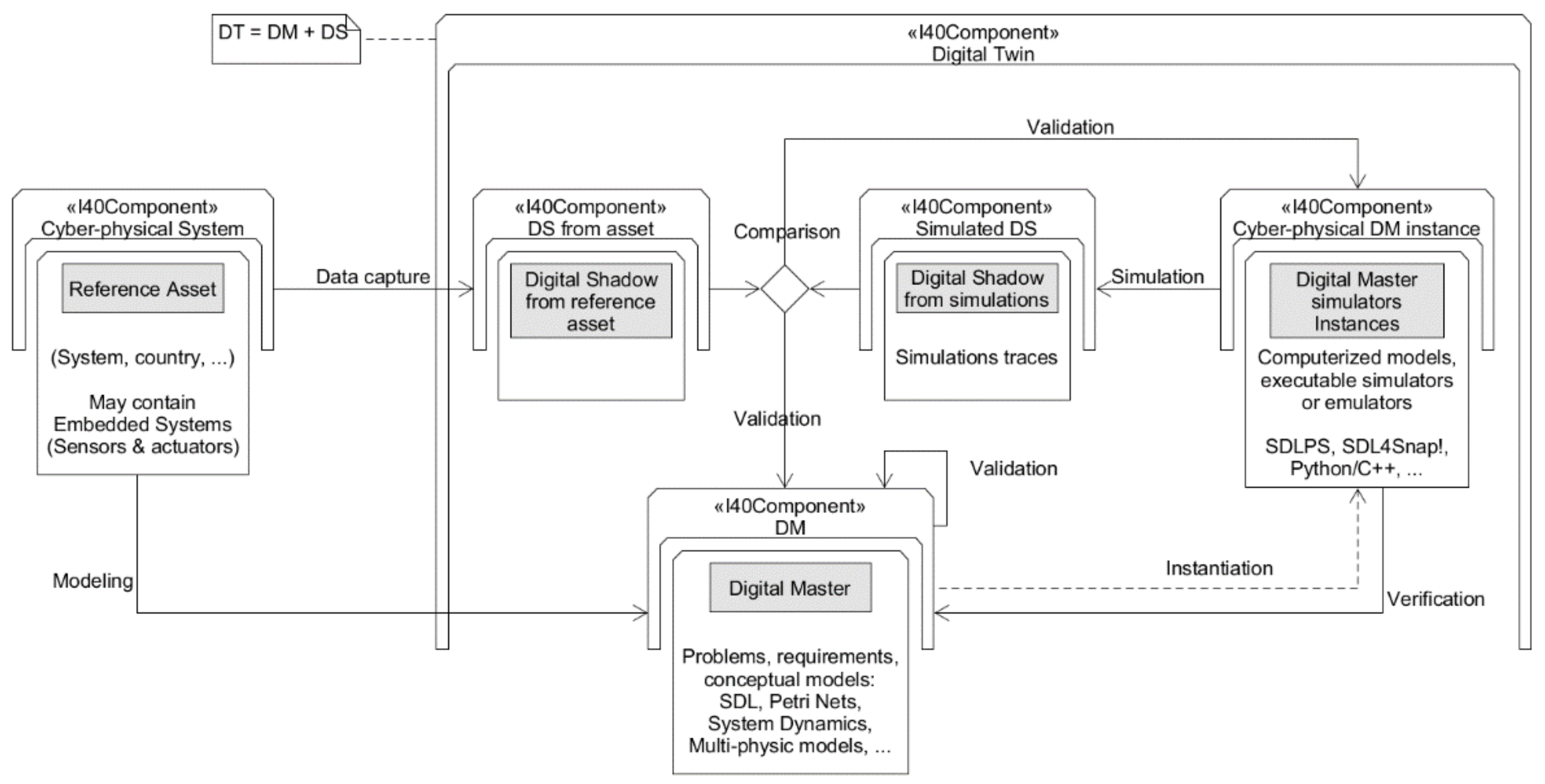
A Digital Twin Approach
2. Materials and Methods
2.1. System Dynamics Model
2.2. Python Model
2.3. The SDL Model
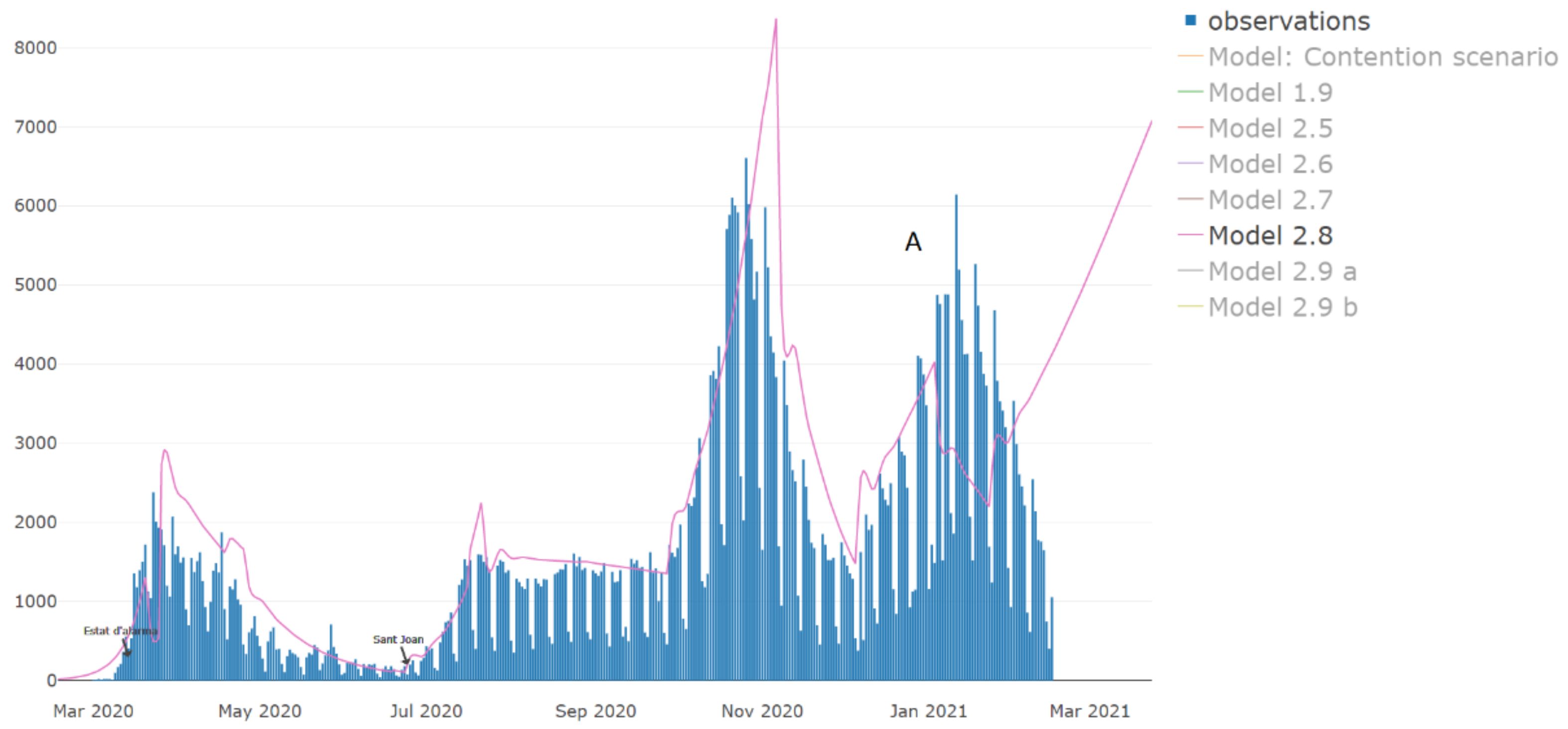
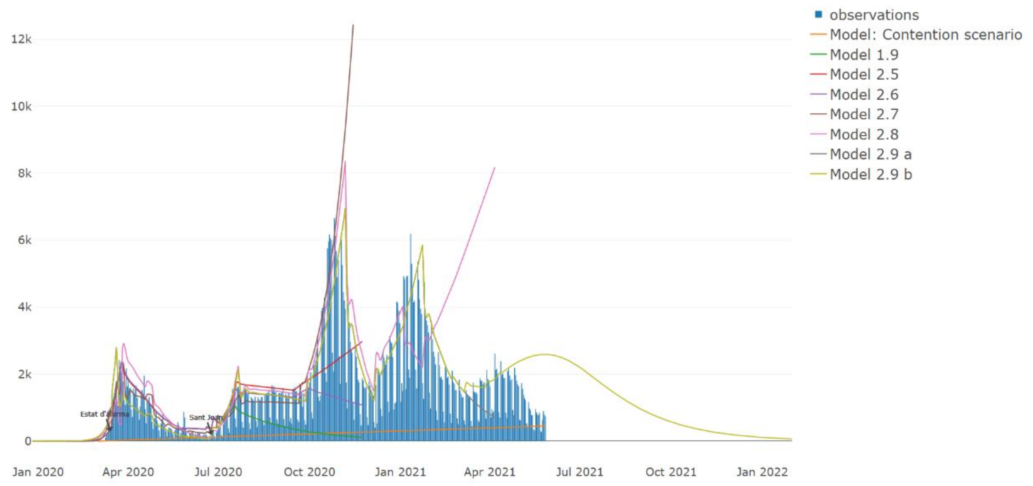
3. Results
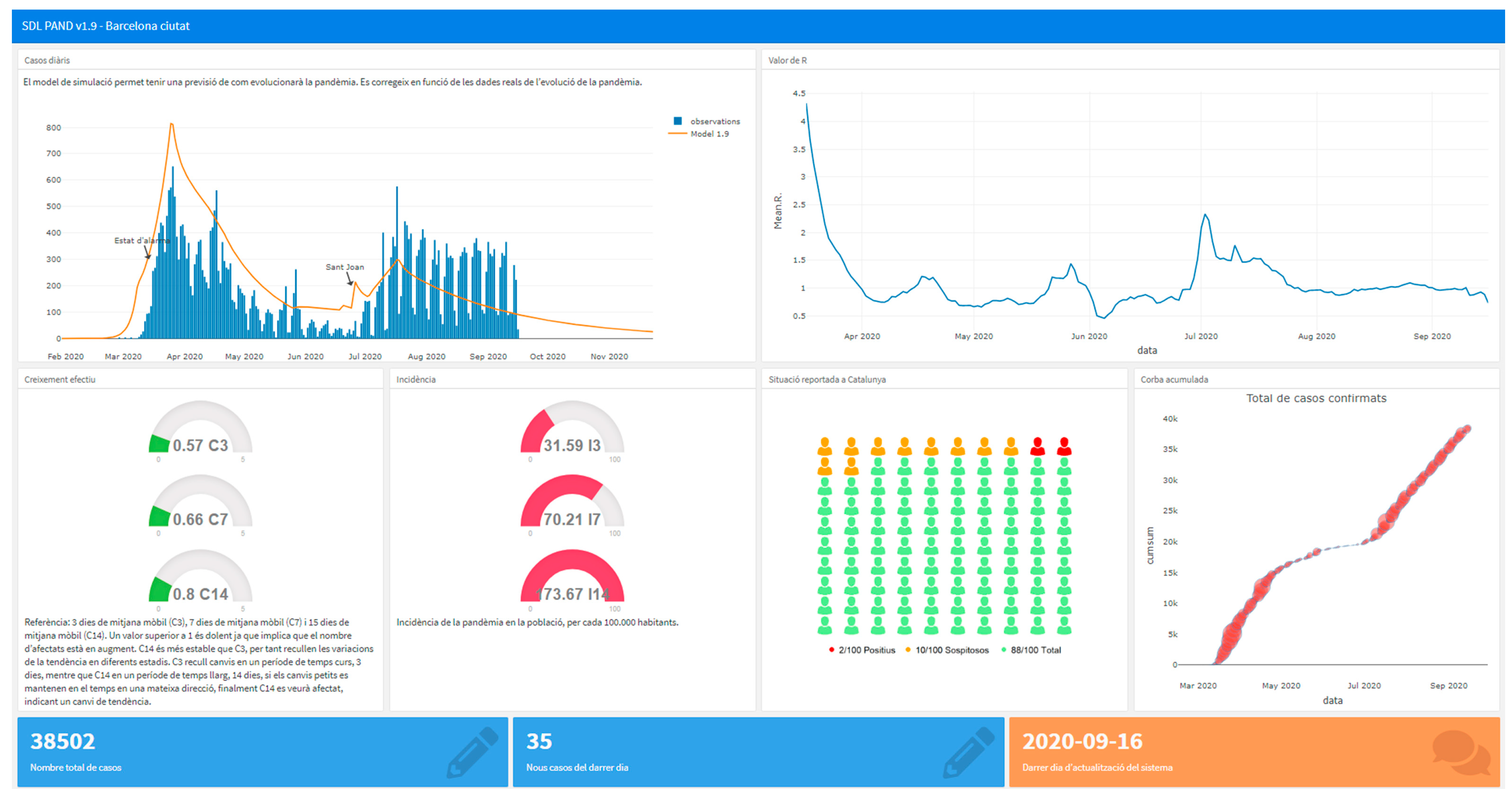
3.1. Models Coding and Calibration
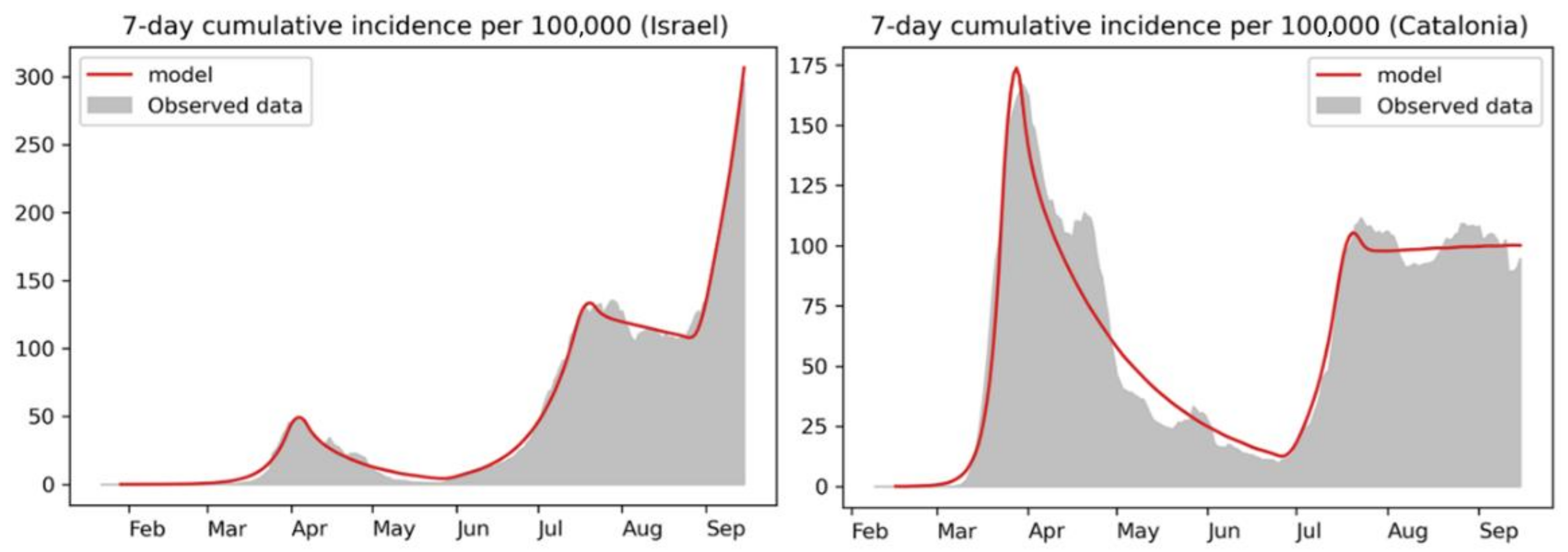
3.2. Second Wave Calibration
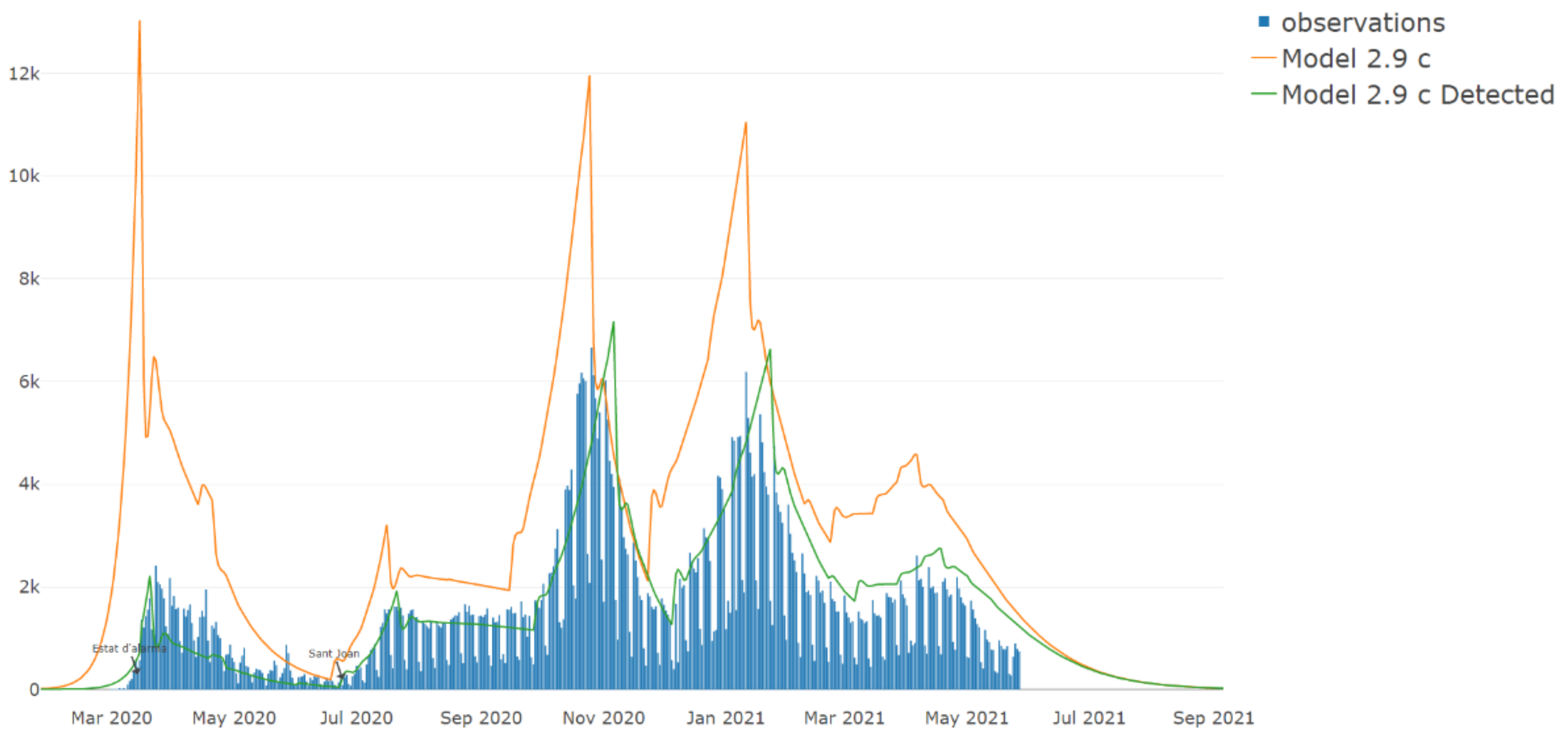
3.3. Third-Wave Calibration
4. Discussion
5. Conclusions
Author Contributions
Funding
Institutional Review Board Statement
Informed Consent Statement
Data Availability Statement
Acknowledgments
Conflicts of Interest
Appendix A. SDL
 This element defines the initial condition for a PROCESS diagram.
 The PROCESS must always start in a STATE, and this owns a name.
 The PROCESS starts an execution when an INPUT receives the SIGNAL for this INPUT. All the STATES can own several different INPUTS to work with the different SIGNALS one can receive.
 This element allows the creation of an AGENT.
 To interpret a piece of code, we can use the TASK element. In our approach, we can use C on this element.
 To send a SIGNAL, we must use the OUTPUT element. We can also add parameters to the SIGNALS and describe the destination if ambiguity about the signal destination exists. We can direct the communication specifying destinations using a PROCESS identifier (PId), an identifier that must own all the PROCESS. Also, we can send using the sentence via path. We can use four PId expressions: (i) self, an agent’s own identity; (ii) parent, the agent that created the agent (Null for initial agents); (iii) offspring, the most recent agent created by the agent; (iv) sender, the agent that sent the last signal input (null before any signal received). Also, we can use {CUR_CELLS} and {ALL_CELL} to send the information to a specific cell of the CA.
 To define a bifurcation, a decision point, we can use the DECISION.
 .
.References
- Anderson, R. Discussion: The Kermack-McKendrick epidemic threshold theorem. Bull. Math. Biol. 1991, 53, 3–32. [Google Scholar] [CrossRef]
- Wynants, L.; van Calster, B.; Collins, G.S.; Riley, R.D.; Heinze, G.; Schuit, E.; Bonten, M.M.J.; Dahly, D.L.; Damen, J.A.; Debray, T.P.A.; et al. Prediction models for diagnosis and prognosis of covid-19: Systematic review and critical appraisal. BMJ 2020, 369, m1328. [Google Scholar] [CrossRef] [Green Version]
- Nava, A.; Papa, A.; Rossi, M.; Giuliano, D. Analytical and cellular automaton approach to a generalized SEIR model for infection spread in an open crowded space. Phys. Rev. Res. 2020, 2, 043379. [Google Scholar] [CrossRef]
- Chen, W.; Zhang, N.; Wei, J.; Yen, H.-L.; Li, Y. Short-range airborne route dominates exposure of respiratory infection during close contact. Build. Environ. 2020, 176, 106859. [Google Scholar] [CrossRef]
- Fonseca i Casas, P.; García i Carrasco, V.; Garcia i Subirana, J. SEIRD COVID-19 Formal Characterization and Model Comparison Validation. Appl. Sci. 2020, 10, 5162. [Google Scholar] [CrossRef]
- Ndaïrou, F.; Area, I.; Nieto, J.J.; Silva, C.J.; Torres, D.F. Fractional model of COVID-19 applied to Galicia, Spain and Portugal. Chaos Solitons Fractals 2021, 144, 110652. [Google Scholar] [CrossRef] [PubMed]
- Ogden, N.H.; Fazil, A.; Arino, J.; Berthiaume, P.; Fisman, D.N.; Greer, A.L.; Ludwig, A.; Ng, V.; Tuite, A.R.; Turgeon, P.; et al. Modelling scenarios of the epidemic of COVID-19 in Canada. Can. Commun. Dis. Rep. 2020, 46, 198–204. [Google Scholar] [CrossRef]
- Faniran, T.; Bakare, E.; Potucek, R.; Ayoola, E. Global and Sensitivity Analyses of Unconcerned COVID-19 Cases in Nigeria: A Mathematical Modeling Approach. WSEAS Trans. Math. 2021, 20, 218–234. [Google Scholar] [CrossRef]
- Arenas, A.; Cota, W.; Gómez-Gardeñes, J.; Gómez, S.; Granell, C.; Matamalas, J.T.; Soriano-Paños, D.; Steinegger, B. Modeling the Spatiotemporal Epidemic Spreading of COVID-19 and the Impact of Mobility and Social Distancing Interventions. Phys. Rev. X 2020, 10, 041055. [Google Scholar] [CrossRef]
- Lymperopoulos, I.N. SIR-Neurodynamical epidemic modeling of infection patterns in social networks. Expert Syst. Appl. 2021, 165, 113970. [Google Scholar] [CrossRef]
- Li, Y.; Campbell, H.; Kulkarni, D.; Harpur, A.; Nundy, M.; Wang, X.; Nair, H. The temporal association of introducing and lifting non-pharmaceutical interventions with the time-varying reproduction number (R) of SARS-CoV-2: A modelling study across 131 countries. Lancet Infect. Dis. 2021, 21, 193–202. [Google Scholar] [CrossRef]
- Flaxman, S.; Mishra, S.; Gandy, A.; Unwin, H.J.T.; Mellan, T.A.; Coupland, H.; Whittaker, C.; Zhu, H.; Berah, T.; Eaton, J.W.; et al. Estimating the effects of non-pharmaceutical interventions on COVID-19 in Europe. Nature 2020, 584, 257–261. [Google Scholar] [CrossRef] [PubMed]
- Ding, Y.; Huang, R.; Shao, N. Time Series Forecasting of US COVID-19 Transmission. Altern. Ther. Health Med. 2021, 27, 4–11. [Google Scholar] [PubMed]
- Maleki, M.; Mahmoudi, M.R.; Wraith, D.; Pho, K.-H. Time series modelling to forecast the confirmed and recovered cases of COVID-19. Travel Med. Infect. Dis. 2020, 37, 101742. [Google Scholar] [CrossRef]
- Vasiljeva, M.; Neskorodieva, I.; Ponkratov, V.; Kuznetsov, N.; Ivlev, V.; Ivleva, M.; Maramygin, M.; Zekiy, A. A Predictive Model for Assessing the Impact of the COVID-19 Pandemic on the Economies of Some Eastern European Countries. J. Open Innov. Technol. Mark. Complex. 2020, 6, 92. [Google Scholar] [CrossRef]
- Deb, P.; Furceri, D.; Ostry, J.; Tawk, N. The Effect of Containment Measures on the COVID-19 Pandemic. IMF Work. Pap. 2020, 20, 166. [Google Scholar] [CrossRef]
- Chen, S.; Prettner, K.; Kuhn, M.; Bloom, D.E. The economic burden of COVID-19 in the United States: Estimates and projections under an infection-based herd immunity approach. J. Econ. Ageing 2021, 20, 100328. [Google Scholar] [CrossRef]
- Sargent, R.G. Verification and Validation of Simulation Models. In Proceedings of the 2007 Winter Simulation Conference, Washington, WA, USA, 9–12 December 2007; pp. 124–137. [Google Scholar]
- Leiva, J.; Fonseca i Casas, P.; Ocaña, J. Modeling anesthesia and pavilion surgical units in a Chilean hospital with Specification and Description Language. Simulation 2013, 89, 1020–1035. [Google Scholar] [CrossRef]
- Vynnycky, E.; White, R. An Introduction to Infectious Disease Modelling; Oxford University Press: Oxford, UK, 2010; ISBN 978-0198565765. [Google Scholar]
- Fonseca i Casas, P.; Garcia i Subirana, J.; Garcia i Carrasco, V.; Silva de Barcellos, J.L.; Roma, J.; Pi, X. SDL Cellular Automaton COVID-19 conceptualization. In Proceedings of the 12th System Analysis and Modelling Conference on ZZZ; ACM: New York, NY, USA, 2020; pp. 144–153. [Google Scholar]
- Grieves, M.; Vickers, J. Digital Twin: Mitigating Unpredictable, Undesirable Emergent Behavior in Complex Systems. In Transdisciplinary Perspectives on Complex Systems; Springer: Berlin, Germany, 2017; pp. 85–113. [Google Scholar]
- Kritzinger, W.; Karner, M.; Traar, G.; Henjes, J.; Sihn, W. Digital Twin in manufacturing: A categorical literature review and classification. IFAC-PapersOnLine 2018, 51, 1016–1022. [Google Scholar] [CrossRef]
- Stark, R.; Kind, S.; Neumeyer, S. Innovations in digital modelling for next generation manufacturing system design. CIRP Ann. 2017, 66, 169–172. [Google Scholar] [CrossRef]
- Sherratt, E.; Ober, I.; Gaudin, E.; Fonseca i Casas, P.; Kristoffersen, F. SDL—The IoT Language. In Lecture Notes in Computer Science (Including Subseries Lecture Notes in Artificial Intelligence and Lecture Notes in Bioinformatics); Springer: Berlin/Heidelberg, Germany, 2015; Volume 9369, pp. 27–41. ISBN 9783319249117. [Google Scholar]
- Generalitat de Catalunya. Registre de Casos de COVID-19 Realitzats a Catalunya. Segregació per Sexe i Edat. Available online: https://analisi.transparenciacatalunya.cat/en/Salut/Registre-de-casos-de-COVID-19-realitzats-a-Catalun/qwj8-xpvk (accessed on 21 February 2021).
- Robinson, S.; Brooks, R.J. Independent Verification and Validation of an Industrial Simulation Model. Simulation 2009, 86, 405–416. [Google Scholar] [CrossRef]
- SciPy. scipy.optimize.dual_annealing. Available online: https://docs.scipy.org/doc/scipy/reference/generated/scipy.optimize.dual_annealing.html (accessed on 21 May 2021).
- Anastassopoulou, C.; Russo, L.; Tsakris, A.; Siettos, C. Data-based analysis, modelling and forecasting of the COVID-19 outbreak. PLoS ONE 2020, 15, e0230405. [Google Scholar] [CrossRef] [Green Version]
- Xiang, Y.; Gubian, S.; Suomela, B.; Hoeng, J. Generalized Simulated Annealing for Global Optimization: The GenSA Package an Application to Non-Convex Optimization in Finance and Physics. R J. 2013, 5, 13–28. [Google Scholar] [CrossRef] [Green Version]
- Pollán, M.; Pérez-Gómez, B.; Pastor-Barriuso, R.; Oteo, J.; Hernán, M.A.; Perez-Olmeda, M.; Sanmartín, J.L.; Fernández-García, A.; Cruz, I.; de Larrea, N.F.; et al. Prevalence of SARS-CoV-2 in Spain (ENE-COVID): A nationwide, population-based seroepidemiological study. Lancet 2020, 396, 535–544. [Google Scholar] [CrossRef]
- Taylor, L. Study Highlights Costa del Sol’s Malaga as One of the Best Quarantined Cities in Spain During Phase 0. Available online: https://www.euroweeklynews.com/2020/05/14/study-highlights-costa-del-sols-malaga-as-one-of-the-best-quarantined-cities-in-spain-during-phase-0/ (accessed on 12 July 2021).
- Ministerio de Sanidad estudio Ene-Covid19: Primera Ronda. Available online: https://www.mscbs.gob.es/ciudadanos/ene-covid/docs/ESTUDIO_ENE-COVID19_PRIMERA_RONDA_INFORME_PRELIMINAR.pdf (accessed on 14 July 2021).
- Ministerio de Sanidad Estudio Ene-Covid19: Segunda Ronda. Available online: https://www.mscbs.gob.es/ciudadanos/ene-covid/docs/ESTUDIO_ENE-COVID19_SEGUNDA_RONDA_INFORME_PRELIMINAR.pdf (accessed on 14 July 2021).
- Ministerio de Sanidad Estudio Ene-Covid: Informe Final. Available online: https://www.mscbs.gob.es/ciudadanos/ene-covid/docs/ESTUDIO_ENE-COVID19_INFORME_FINAL.pdf (accessed on 14 July 2021).
- Ministerio de Sanidad Estudio Ene-Covid: Cuarta Ronda. Available online: https://www.mscbs.gob.es/gabinetePrensa/notaPrensa/pdf/15.12151220163348113.pdf (accessed on 14 July 2021).
- Jung, C.-Y.; Park, H.; Kim, D.W.; Choi, Y.J.; Kim, S.W.; Chang, T.I. Clinical Characteristics of Asymptomatic Patients with COVID-19: A Nationwide Cohort Study in South Korea. Int. J. Infect. Dis. 2020, 99, 266–268. [Google Scholar] [CrossRef] [PubMed]
- Nishiura, H.; Kobayashi, T.; Miyama, T.; Suzuki, A.; Jung, S.-M.; Hayashi, K.; Kinoshita, R.; Yang, Y.; Yuan, B.; Akhmetzhanov, A.R.; et al. Estimation of the asymptomatic ratio of novel coronavirus infections (COVID-19). Int. J. Infect. Dis. 2020, 94, 154–155. [Google Scholar] [CrossRef] [PubMed]
- Reed, R. SDL-2000 for New Millennium Systems. Telektronikk 2000, 96, 20–35. [Google Scholar]
- Doldi, L. SDL Illustrated—Visually Design Executable Models, 1st ed.; TMSO Systems, Ed.; TMSO Systems: Old Main, PA, USA, 2001; ISBN 978-2951660007. [Google Scholar]
- Campbell, F.; Archer, B.; Laurenson-Schafer, H.; Jinnai, Y.; Konings, F.; Batra, N.; Pavlin, B.; Vandemaele, K.; van Kerkhove, M.D.; Jombart, T.; et al. Increased transmissibility and global spread of SARS-CoV-2 variants of concern as at June 2021. Eurosurveillance 2021, 26, 2100509. [Google Scholar] [CrossRef]
- Agencias Catalunya Levanta a Partir del Lunes la Prohibición de Celebrar Fiestas Mayores. Available online: https://www.lavanguardia.com/vida/20210604/7504929/catalunya-levanta-lunes-prohibicion-celebrar-fiestas-mayores-procicat-coronavirus-covid.html (accessed on 4 June 2021).


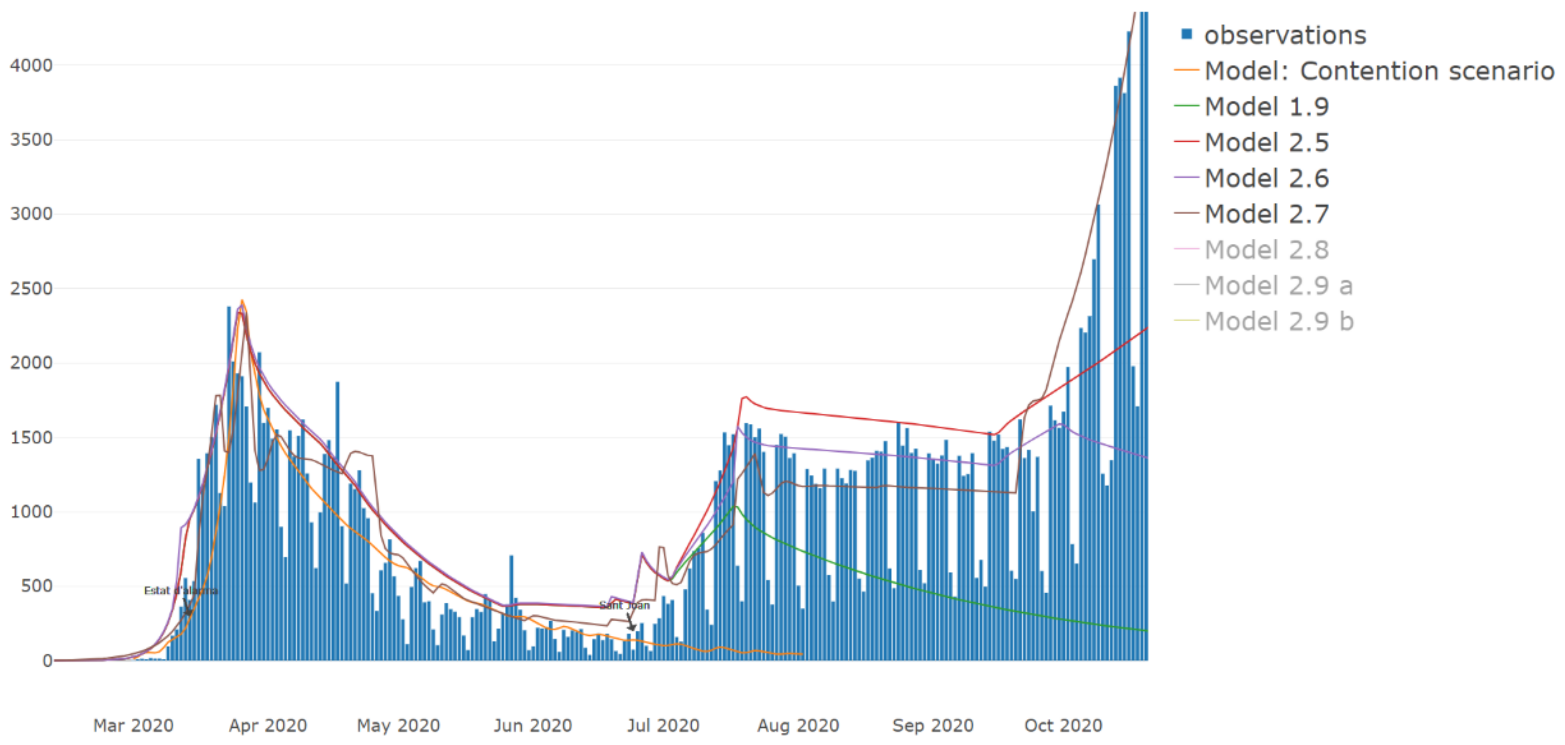
| Model Number | Description | Valid (at the Time of Writing This Paper) |
|---|---|---|
| 1.9 | The initial model contains the initial growth and the total lockdown | No, the total lockdown was open. |
| 2.5 | Optimistical return to normality (schools and work). | No |
| 2.6 | Increase online learning and teleworking. | No |
| 2.7 | Pessimistic return to normality. | No |
| 2.8 | More NPIs application. | No |
| 2.9 | Readjusted the effect of the holidays and January restraints added. Adding the effects of the vaccination on the population. | Yes |
| Id. | Code | Description | Population |
|---|---|---|---|
| 6100 | LL | Lleida | 362,850 |
| 6200 | CT | Camp de Tarragona | 607,999 |
| 6300 | TE | Terres de l’Ebre | 176,817 |
| 6400 | GR | Girona | 861,753 |
| 6700 | CC | Catalunya Central | 526,959 |
| 7100 | AA | Vall d’Aran | 67,277 |
| 7801 | BS | Barcelona Sud | 1,370,709 |
| 7802 | BN | Barcelona Nord | 1,986,032 |
| 7803 | BC | Barcelona Ciutat | 1,693,449 |
| All | CAT | Catalunya | 7,653,845 |
| Event | Date (2020) | β | % Det | % Conf | NPIs |
|---|---|---|---|---|---|
| 1 | 29 January | 1.2 | 0.1 | 0% | First infected |
| 2 | 08 Febrary | 1.2 | 0.25 | 0% | Initial tests |
| 3 | 15 March | 0.6 | 0.45 | 35% | Confinement |
| 4 | 23 March | 0.24 | 0.45 | 35% | Air space closes |
| 5 | 13 April | 0.2 | 0.45 | 25% | Workers partial comeback |
| 6 | 20 April | 0.18 | 0.45 | 25% | Free masks |
| 7 | 25 May | 0.18 | 0.45 | 25% | Phase 1 for some regions |
| 8 | 18 June | 0.18 | 0.54 | 0% | Phase 3 for BCN |
| 9 | 24 June | 1.2 | 0.54 | 0% | National day |
| 10 | 25 June | 0.18 | 0.54 | 0% | Phase 3 for BCN |
| 11 | 02 July | 0.3 | 0.54 | 0% | New normality |
| 12 | 17 July | 0.21 | 0.54 | 0% | Summer plateau |
| 13 | 15 September | 0.24 | 0.7 | 0% | School returns |
| Regime | Israel | S. Korea | Catalonia |
|---|---|---|---|
| First outbreak | 0.55 | 0.95 | 0.95 |
| Lockdown | 0.12 | 0.09 | 0.15 |
| Summer outbreak | 0.34 | (*) | 0.43 |
| Summer plateau | 0.20 | (*) | 0.20 |
| Reopening outbreak | 0.33 | 0.48 | 0.30 (**) |
| Partial lockdown | (?) | 0.12 | (?) |
| Event | Date | β | %Det | % Conf | Description Event |
|---|---|---|---|---|---|
| 1 | 01 December 2019 | - | - | - | Start of simulation |
| 2 | 01 December 2019 | 0.81 | 0 | 0 | - |
| 3 | 11 December 2019 | 0.81 | 0.11 | 0 | Pandemic Beginning |
| 4 | 15 March 2020 | 0.81 | 0.17 | 0 | Confinement |
| 5 | 15 March 2020 | 0.81 | 0.17 | 0.35 | Confinement |
| 6 | 15 March 2020 | 0.25 | 0.17 | 0.35 | Confinement |
| 7 | 13 April 2020 | 0.25 | 0.17 | 0.2 | Workers partial comeback |
| 8 | 20 April 2020 | 0.16 | 0.17 | 0.2 | Free Masks |
| 9 | 06 May 2020 | 0.16 | 0.18 | 0.2 | Phase 1 for some regions |
| 10 | 01 June 2020 | 0.16 | 0.25 | 0.2 | Phase 3 for some regions |
| 11 | 18 June 2020 | 0.465 | 0.25 | 0.2 | Phase 3 for BCN |
| 12 | 18 June 2020 | 0.465 | 0.25 | 0 | Phase 3 for BCN |
| 13 | 22 June 2020 | 0.465 | 0.6 | 0 | New normality |
| 14 | 16 July 2020 | 0.21 | 0.6 | 0 | Summer plateau |
| 15 | 15 September 2020 | 0.34 | 0.6 | 0 | School returns |
| 16 | 20 October 2020 | 0.34 | 0.6 | 0.03 | University online (2) |
| 17 | 25 October 2020 | 0.34 | 0.6 | 0.1 | Movement and restaurants restrictions |
| 18 | 25 October 2020 | 0.15 | 0.6 | 0.1 | Movement and restaurants restrictions |
| 19 | 23 November 2020 | 0.3 | 0.6 | 0.1 | Reopening restaurants |
| 20 | 23 November 2020 | 0.3 | 0.6 | 0.03 | Reopening restaurants |
| 21 | 23 December 2020 | 0.21 (0.3) (1) | 0.6 | 0.03 | Holidays |
| 22 | 11 January 2021 | 0.3 | 0.6 | 0.03 | Schools Returns |
Publisher’s Note: MDPI stays neutral with regard to jurisdictional claims in published maps and institutional affiliations. |
© 2021 by the authors. Licensee MDPI, Basel, Switzerland. This article is an open access article distributed under the terms and conditions of the Creative Commons Attribution (CC BY) license (https://creativecommons.org/licenses/by/4.0/).
Share and Cite
Fonseca i Casas, P.; Garcia i Subirana, J.; García i Carrasco, V.; Pi i Palomés, X. SARS-CoV-2 Spread Forecast Dynamic Model Validation through Digital Twin Approach, Catalonia Case Study. Mathematics 2021, 9, 1660. https://doi.org/10.3390/math9141660
Fonseca i Casas P, Garcia i Subirana J, García i Carrasco V, Pi i Palomés X. SARS-CoV-2 Spread Forecast Dynamic Model Validation through Digital Twin Approach, Catalonia Case Study. Mathematics. 2021; 9(14):1660. https://doi.org/10.3390/math9141660
Chicago/Turabian StyleFonseca i Casas, Pau, Joan Garcia i Subirana, Víctor García i Carrasco, and Xavier Pi i Palomés. 2021. "SARS-CoV-2 Spread Forecast Dynamic Model Validation through Digital Twin Approach, Catalonia Case Study" Mathematics 9, no. 14: 1660. https://doi.org/10.3390/math9141660
APA StyleFonseca i Casas, P., Garcia i Subirana, J., García i Carrasco, V., & Pi i Palomés, X. (2021). SARS-CoV-2 Spread Forecast Dynamic Model Validation through Digital Twin Approach, Catalonia Case Study. Mathematics, 9(14), 1660. https://doi.org/10.3390/math9141660