Nonlinear Compartment Models with Time-Dependent Parameters

Abstract

A nonlinear compartment model generates a semi-process on a simplex and may have an arbitrarily complex dynamical behaviour in the interior of the simplex. Nonetheless, in applications nonlinear compartment models often have a unique asymptotically stable equilibrium attracting all interior points. Further, the convergence to this equilibrium is often wave-like and related to slow dynamics near a second hyperbolic equilibrium on the boundary. We discuss a generic two-parameter bifurcation of this equilibrium at a corner of the simplex, which leads to such dynamics, and explain the wave-like convergence as an artifact of a non-smooth nearby system in $C^0$-topology, where the second equilibrium on the boundary attracts an open interior set of the simplex. As such nearby idealized systems have two disjoint basins of attraction, they are able to show rate-induced tipping in the non-autonomous case of time-dependent parameters, and induce phenomena in the original systems like, e.g., avoiding a wave by quickly varying parameters. Thus, this article reports a quite unexpected path, how rate-induced tipping can occur in nonlinear compartment models.

1. Introduction

Nonlinear compartment models [1], which in the autonomous case generate semi-dynamical systems on a simplex, have been used in many areas of science, particularly in life sciences, to study transmissions among different compartments of a system. In this article, we are mainly interested in nonlinear compartment models with time-dependent parameters, i.e., in the non-autonomous case, in which a semi-process on a simplex is generated. For certain non-autonomous systems [2] which are not compartment models, it is known from the literature that tipping phenomena different from bifurcations can occur. Particularly, rate-induced tipping caused by a fast parameter change and leading to a drastic change in the behaviour of the system has been studied in climate models [3], in two-dimensional models of ecosystems [4], in predator–prey systems [5], and in chaotic systems [6]. Indicators for rate-induced tipping have been studied [7], and rate-induced tipping in systems with discrete time have been discussed [8].

The main mechanism for rate-induced tipping in smooth systems on ${\mathbb{R}}^n$ is basin instability, where due to a parameter change the disjoint basins of attraction of two local attractors change so fast that the actual state tips from one to the other local attractor. However, this mechanism seems to fail in many nonlinear compartment models due to global asymptotic stability results. For example, in many models of mathematical epidemology, if the basic reproduction number $R_0$ satisfies $R_0<1$, then the disease-free equilibrium at a corner of the simplex is globally asymptotically stable and the disease will die out, while for $R_0>1$, the endemic equilibrium attracts all interior points and the disease will become endemic. Particularly, in such models there are no two disjoint basins of attraction, and rate-induced tipping cannot be caused by basin instability.

Yet, in epidemiological systems, it seems to have a drastic effect if measures to contain an epidemic are taken sufficiently fast, i.e., the rate of a parameter change seems to play an important role. Further, the occurrence of epidemic waves indicates that there should be trajectories connecting the endemic equilibrium and the disease-free equilibrium. Particularly, it should be possible that a disease dies out just by establishing measures to contain the disease sufficiently fast, while if containment is too slow the disease becomes endemic. This article shows mathematically rigorously that there are nonlinear compartment models with this behaviour. However, these models have to be non-smooth near the disease-free equilibrium, and this seems to be the reason why rate-induced tipping is not visible in classical studies of nonlinear compartment models and has not been studied in literature.

More precisely, the main aim of this article is to show that rate-induced tipping caused by basin instability can occur in nonlinear compartment models, which are continuous but non-smooth near a boundary equilibrium point attracting an open interior set, and which have another locally asymptotically stable equilibrium in the interior. In the case of epidemiology, in such idealized systems epidemic behaviour, where the disease dies out, and endemic behaviour, where the disease remains, do not only coexist, but can even interchange during time in dependence on the measures undertaken to contain the disease. Moreover, artifacts of this behaviour in idealized systems can also be seen in the original system, and even in the autonomous case the dynamics of the idealized systems may explain the long-wave-like convergence to the locally asymptotically stable equilibrium in the interior. While in the context of epidemiology such idealized systems have been qualitatively discussed in [9], here we explicitly describe the quantitative construction of such non-smooth systems, and by studying the behaviour along nullclines, we prove that the dynamics are as claimed. Moreover, we discuss that these dynamics occur generically after a two-parameter bifurcation of an equilibrium at a corner of the simplex.

2. Preliminaries

Compartment models with continuous time are ODEs such that all quantities remain non-negative during time and their total number is conserved, i.e., the ODEs have to leave positively invariant a simplex. In this article, we assume that all quantities are given in percentages, i.e., they are normed so that the total number is 1, and correspondingly the simplex is a probability simplex.

Definition 1.

A compartment model with $n+1$ compartments is an ODE system $\dot{x}\left(t\right)=f(t,x\left(t\right))$ generating a semi-process on the n-dimensional probability simplex ${{\Sigma }}^n$: = $\{x\in {\mathbb{R}}^{n+1}|x\ge 0,1^{T}x=1\}\subset {\mathbb{R}}^{n+1}$.

Let us recall that a semi-process on ${{\Sigma }}^n$ is a family of continuous maps ${{\Phi }}^{t,s}:{{\Sigma }}^n\to {{\Sigma }}^n$, $s\le t$, such that ${{\Phi }}^{t,t}={Id}_{{{\Sigma }}^n}$ for all $t\in \mathbb{R}$ and the cocycle condition ${{\Phi }}^{t,r}={{\Phi }}^{t,s}\circ {{\Phi }}^{s,r}$ holds for all $r\le s\le t$. An ODE $\dot{x}\left(t\right)=f(t,x\left(t\right))$ with a time-dependent vector field $f:\mathbb{R}\times {\mathbb{R}}^{n+1}\to {\mathbb{R}}^{n+1}$ admitting locally unique solutions generates such a semi-process ${\Phi }$ on ${{\Sigma }}^n$ by ${{\Phi }}^{t,s}{x}_s:=x\left(t\right)$ for the unique solution $x(·)$ starting at the point $x_s$ at time s, if the probability simplex ${{\Sigma }}^n$ is positively invariant, and this is the case if

(A1)

$f_i(t,x)\ge 0$ holds for every $x\ge 0$ with $1^{T}x=1$ and $x_i=0$, and every $t\in \mathbb{R}$,

(A2)

$1^{T}f(t,x)=0$ holds for every $x\in {{\Sigma }}^n$ and every $t\in \mathbb{R}$.

Due to conservation $1^{T}x\left(t\right)=1$ for all $t\in \mathbb{R}$, every compartment model can be reduced by one dimension to an n-dimensional ODE $\dot{\widehat{x}}=\widehat{f}(t,\widehat{x})$ on the image ${\widehat{{\Sigma }}}^n$: = $\{\widehat{x}\in {\mathbb{R}}^n|\widehat{x}\ge 0,1^T\widehat{x}\le 1\}$ of the diffeomorphism from ${{\Sigma }}^n$ onto ${\widehat{{\Sigma }}}^n$ given by $x=(x_1,\cdots ,x_n,x_{n+1})\mapsto (x_1,\cdots ,x_n)=\widehat{x}$ with inverse $\widehat{x}\mapsto (\widehat{x},1-1^T\widehat{x})=x$, i.e., by eliminating $x_{n+1}=1-{\sum }_{i=1}^n{x}_i$ from the ODE. The assumptions (A1) and (A2) then translate into

(A1)’

${\widehat{f}}_i(t,\widehat{x})\ge 0$ holds for every $\widehat{x}\ge 0$ with $1^T\widehat{x}<1$ and ${\widehat{x}}_i=0$ and every $t\in \mathbb{R}$,

(A2)’

${\sum }_{i=1}^n{\widehat{f}}_i(t,\widehat{x})\le 0$ holds for every $\widehat{x}\ge 0$ with $1^T\widehat{x}=1$, and every $t\in \mathbb{R}$,

Furthermore, this definition of compartmental systems is used, e.g., in [1].

In this article, we are particularly interested in compartment models

$$\dot{x}\left(t\right)=f(x\left(t\right),\lambda \left(t\right))$$

(1)

with time-dependent parameters $\lambda \left(t\right)\in {\Lambda }$ in a finite-dimensional vector space ${\Lambda }$, where the vector field $f:{\mathbb{R}}^{n+1}\times {\Lambda }\to {\mathbb{R}}^{n+1}$ depends on time only due to its dependence on the parameter. Further, we assume that the system (1) is driven, i.e., the total system for the state $x\left(t\right)$ and the parameter $\lambda \left(t\right)$ can be written in skew-product form

$$\begin{array}{cc}\hfill \dot{x}\left(t\right)=& f\left(x\right(t),\lambda (t\left)\right)\hfill \\ \hfill \dot{\lambda }\left(t\right)=& rg\left(\lambda \right(t\left)\right)\hfill \end{array}$$

(2)

with parameter path induced by a vector field $g\left(\lambda \right)$ on ${\Lambda }$ independent of x. Increasing or decreasing the rate $r>0$ does not change the trace of the parameter path, but just the speed of the parameter change. Additionally, we assume that $\lambda \left(t\right)$ approaches constant values ${\lambda }_{\pm }$ for times $t\to \pm \infty$ with a flat derivative, i.e., $\lambda \left(t\right)$ is a heteroclinic orbit in parameter space connecting ${\lambda }_{\pm }$ and satisfies $\dot{\lambda }\left(t\right)\to 0$ as $t\to \pm \infty$ due to $g\left({\lambda }_{\pm }\right)=0$.

If in (1) the time-dependent parameter $\lambda \left(t\right)$ is replaced by a constant $\lambda$, then we call

$$\dot{x}\left(t\right)=f(x\left(t\right),\lambda )$$

(3)

the corresponding autonomous ODE with frozen parameters. In such a parameter-dependent autonomous ODE, a sudden qualitative change of the behaviour of the system at a threshold $\lambda ={\lambda }_0$ can only occur due to a bifurcation. In fact, by definition, a bifurcation is said to occur at the parameter ${\lambda }_0$ if there are arbitrarily close parameters for which the generated dynamics are not topologically equivalent. In contrast, for the non-autonomous system (1), there are other possibilities for a sudden qualitative change. Particularly, rate-induced tipping may happen, where the system fails to track a continuously changing quasistatic attractor due to a fast rate of change of parameters.

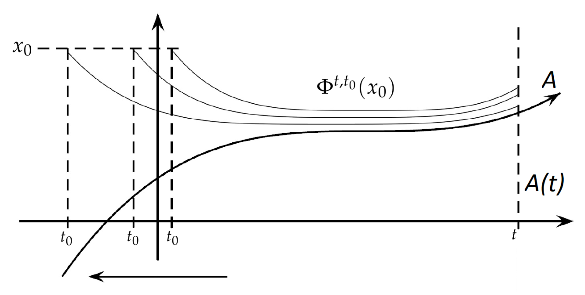
To define the corresponding notions [2], note that the long-time behaviour of a non-autonomous compartment model generating a semi-process ${\Phi }$ on ${{\Sigma }}^n$ is governed by its global pullback attractor, i.e., by the time-dependent family of non-empty compact sets

$$A\left(t\right):=\bigcap _{s\le t}\overline{\bigcup _{r\le s}{{\Phi }}^{t,r}\left(D\right)},$$

(4)

with $D:={{\Sigma }}^n$ chosen to be the whole state space. By definition, $A\left(t\right)$ consists of all values of solutions at time t originating from D for times $s\to -\infty$, i.e., $A\left(t\right)$ is a kind of non-autonomous $\omega$-limit set of orbits originating from D, see Figure 1 for a symbolic visualization.

Figure 1. A symbolic visualization of the pullback attractor [2], showing that $A\left(t\right)$ consists of all values of solutions at time t originating at times $t_0\to -\infty$, and the pullback attractor A is the family of all these $A\left(t\right)$.

The global pullback attractor is the minimal closed set which attracts all subsets $B\subset {{\Sigma }}^n$ at time $-\infty$, i.e., $\underset{s\to -\infty }{\text{lim}}dist({{\Phi }}^{t,s}\left(B\right),A\left(t\right))=0$ holds for every subset $B\subset {{\Sigma }}^n$, and it is invariant, i.e., ${{\Phi }}^{t,s}A\left(s\right)=A\left(t\right)$ holds for all $s\le t$. In the autonomous case, where ${{\Phi }}^{t,s}={{\Phi }}^{t-s}$ is a continuous dynamical system on ${{\Sigma }}^n$ and the vector field f in the generating ODE $\dot{x}\left(t\right)=f\left(x\left(t\right)\right)$ does not depend on time, also the global pullback attractor does not depend on time, i.e., $A\left(t\right)=A$ is a constant set, and A is identical with the global attractor of the autonomous dynamical system on ${{\Sigma }}^n$.

If D in (4) is not chosen as whole space ${{\Sigma }}^n$, but replaced by a locally pullback absorbing family of time dependent sets $D\left(r\right)$, i.e., by a family such that there exists a sufficiently small distance $\epsilon >0$ and a sufficiently large time $T>0$ with ${{\Phi }}^{t,r}\left(B_{\epsilon }\left(D\left(r\right)\right)\right)\subset D\left(t\right)$ for all $(t,r)$ satisfying $t\ge r+T$, where the $\epsilon$-neighborhood of $D\subset {{\Sigma }}^n$ is denoted by $B_{\epsilon }\left(D\right):=\{x\in {{\Sigma }}^n|dist(x,D)<\epsilon \}$, then $A\left(t\right)$ is called the local pullback attractor of the absorbing family $D\left(t\right)$. Given a local pullback attractor $A\left(t\right)$, the largest locally pullback absorbing family $D\left(t\right)$ of time-dependent sets such that $A\left(t\right)\subset D\left(t\right)$ is called its time-dependent basin of attraction, and similarly in the autonomous case, where the basin of attraction is independent of time.

The local pullback attractor $A\left(t\right)$ of an absorbing family $D\left(t\right)$ of the non-autonomous system can be compared to the local quasistatic attractors $A\left(\lambda \right(t\left)\right)$ of the autonomous ODE with parameters frozen at time t attracting all points in $D\left(t\right)$.

Definition 2.

For a non-autonomous ODE (1), a local attractor $A\left(\lambda \right)$ of the corresponding autonomous ODE (3) frozen at the parameter λ is called a local quasistatic attractor.

Let us assume that along $\lambda \left(t\right)$ there is no bifurcation in the autonomous system, so that $A\left({\lambda }_{-}\right)$ has a unique continuation $A\left(\lambda \right(t\left)\right)$ for all times t. We are interested in rate-induced tipping, which happens if the the non-autonomous system fails to track $A\left(\lambda \right(t\left)\right)$ due to a fast rate of change r of parameters. More precisely, if the rate $r>0$ is sufficiently small, then the local pullback attractor $A\left(t\right)$ originating from $A\left({\lambda }_{-}\right)$ uniformly tracks $A\left(\lambda \right(t\left)\right)$, i.e., ${sup}_{t\in \mathbb{R}}dist(A\left(t\right),A\left(\lambda \left(t\right)\right))$ is continuous w.r.t. to the rate r on which $\lambda \left(t\right)$ depends by (2) for small $r>0$, and $dist\left(A\right(t),A(\lambda \left(t\right)\left)\right)$ tends to 0 as $t\to \pm \infty$. This property was obtained in [10] and allows to define rate-induced tipping as follows (for an alternative definition see in [11]).

Definition 3.

Under the assumption that along the path $\lambda \left(t\right)$ there is no bifurcation of the local quasistatic attractor $A\left(\lambda \right(t\left)\right)$, we say that at points of discontinuity of $r\mapsto {sup}_{t\in \mathbb{R}}dist(A\left(t\right),A\left(\lambda \left(t\right)\right))$ the system (1) has

• transient (=reversible) rate-induced tipping, if $\underset{t\to \infty }{\text{lim}}dist(A\left(t\right),A\left(\lambda \left(t\right)\right))=0$,
• irreversible rate-induced tipping, if $\underset{t\to \infty }{\text{lim}}dist(A\left(t\right),A\left(\lambda \left(t\right)\right))>0$.

In case of irreversible rate-induced tipping, the local pullback attractor $A\left(t\right)$ may tend for $t\to \infty$ to a local attractor at ${\lambda }_{+}$ different from $A\left({\lambda }_{+}\right)$, while in case of transient rate-induced tipping $A\left(t\right)$ tends for $t\to \infty$ to $A\left({\lambda }_{+}\right)$, but in between $A\left(t\right)$ approaches another local attractor of the autonomous system. Rate-induced tipping is closely related to basin instability, see in [4] ([Definition 5.1]). Particularly, for equilibria the following definition makes sense.

Definition 4.

Suppose $A\left(\lambda \right)$ is a locally asymptotically stable equilibrium of the autonomous frozen ODE (3) for every λ on the chosen parameter path $\lambda \left(t\right)$, and let $B\left(A\right(\lambda \left)\right)$ denote the basin of attraction of $A\left(\lambda \right)$. Then, $A\left(\lambda \right)$ is said to be basin unstable on the parameter path, if there are two ${\lambda }_1,{\lambda }_2$ on the parameter path such that $A\left({\lambda }_1\right)$ is outside the closure of the basin of attraction of $A\left({\lambda }_2\right)$, i.e., $A\left({\lambda }_1\right)\notin \overline{B\left(A\left({\lambda }_2\right)\right)}$.

In fact, basin instability implies the existence of a parameter path along which irreversible rate-induced tipping happens.

Theorem 1

([4]). If a stable equilibrium $A\left(\lambda \right)$ of the autonomous frozen ODE (3) is basin unstable on the parameter path, then there is a time-varying external input $\lambda \left(t\right)$ of sufficiently fast rate that traces out the path and gives irreversible rate-induced tipping from $A\left(\lambda \right(t\left)\right)$ in the non-autonomous system.

Thus, briefly, if the system is in a state where the dynamics are slow, but the actual parameter change is fast, then it may happen that the state may leave the basin of attraction of the continuation $A\left(\lambda \right(t\left)\right)$ of the attractor $A\left({\lambda }_{-}\right)$ and the local pullback attractor $A\left(t\right)$ tends to a different local attractor of the system.

Like in [3,4,5,6], to the best of our knowledge, all systems showing rate-induced tipping studied in literature seem to have the property that irreversible rate-induced tipping is caused by basin instability. Particularly, there are always two disjoint basins of attraction of local quasistatic attractors of the frozen system. However, in smooth nonlinear compartment models there often is only one locally asymptotic stable equilibrium, which attracts all interior points, and although there often is another hyperbolic equilibrium on the boundary of the simplex, there is no way how basin instability can happen. Yet, the main result of this article is that there are nearby nonlinear compartment models w.r.t. $C^0$-topology, which are smooth in the interior of the simplex as well as continuous but non-smooth near a boundary equilibrium point attracting an open interior set. In these so-called idealized systems, rate-induced tipping can happen, and artifacts of rate-induced tipping in the nearby idealized systems can be observed in the original systems. Moreover, we show that there is a two-parameter bifurcation scenario in which this phenomenon occurs generically.

Yet, before we discuss such nonlinear compartment models, let us take a short look on linear compartment models and perturbations, in which the above mentioned property of a single locally asymptotic stable equilibrium attracting all interior points holds true and excludes the possibility of basin instability.

3. Linear Compartment Models

Autonomous linear compartment models $\dot{x}=Ax+b$ with a square matrix A and a vector b necessarily satisfy $b=0$ [1]. Such linear compartment models occur frequently in literature, for example, in ecology.

Example 1.

The neutral theory in ecology [12] models the time evolution of the probability $x_n$ that a species contains n individuals by the linear compartment model

$${\dot{x}}_n=d_{n+1}{x}_{n+1}+b_{n-1}{x}_{n-1}-(b_n+d_n)x_n,n=0,1,2,\cdots$$

(5)

where $b_n$ and $d_n$ represent the probabilities of birth and death, respectively, in a species with n individuals (and $b_{-1}=0=d_0$). While formally this system (5) is an ODE on the infinite-dimensional probability simplex ${{\Sigma }}^{\infty }:=\{x\in l^1\left({\mathbb{N}}_0\right)|\forall n\in {\mathbb{N}}_0:x_n\ge 0,{\sum }_{n=0}^{\infty }{x}_n=1\}$, for simulations the system is usually cut off at N by assuming (5) for $n=0,1,\cdots ,N-1$ and letting $x_N:=1-{\sum }_{n=0}^{N-1}{x}_n$ be the probability that the species has N or more individuals. This results in a linear ODE system on the N-dimensional probability simplex ${{\Sigma }}^N$.

To briefly discuss linear compartment models with constant parameters, let us introduce some notions for matrices, which unfortunately are not uniformly used in literature.

Definition 5.

A matrix $A=\left(a_{ij}\right)\in {\mathbb{R}}^{n\times n}$ is called

1 

Z-matrix, if $a_{ij}\le 0$ holds for $i\ne j$,

2 

Metzler matrix, if $a_{ij}\ge 0$ holds for $i\ne j$, or equivalently $-A$ is a Z-matrix,

3 

M-matrix, if A is a Z-matrix and additionally $\Re \left(\lambda \right)\ge 0$ holds for every eigenvalue λ of A, or equivalently there is a non-negative matrix $B\ge 0$ and a scalar $\alpha \ge \rho \left(B\right)$ such that $A=\alpha E-B$.

A linear ODE $\dot{x}=Ax$ is a linear compartment model, if the generated linear flow is non-negative and leaves the subspace $\{x\in {\mathbb{R}}^n|1^{T}x=1\}$ invariant. A well-known Theorem is the following characterization of linear compartment models, which additionally provides a criterion for the existence of a unique globally asymptotically stable equilibrium in the interior of the simplex.

Theorem 2

([9]). The probability simplex ${{\Sigma }}^{n-1}:=\{x\in {\mathbb{R}}^n|x\ge 0,1^{T}x=1\}$ is positively invariant w.r.t. the linear flow generated by $\dot{x}=Ax$, iff A is a Metzler matrix with $A^{T}1=0$. In this case, $-A$ is a M-matrix with semi-simple eigenvalue 0. If additionally $A=B-\rho \left(B\right)I$ for an irreducible matrix $B\ge 0$, then there is a unique equilibrium in the interior of the simplex, and this equilibrium is globally asymptotically stable.

Example 2.

The matrix $B:=\left(\begin{array}{ccc}0& 0& 0\\ 1& 0& 1\\ 0& 1& 0\end{array}\right)$ is non-negative, but not irreducible. It has eigenvalues $-1,0,1$, thus $A:=B-E$ is a Metzler matrix with simple eigenvalue 0, and $A^{T}1=0$ holds. Nonetheless, $\dot{x}=Ax$ has no equilibrium in the interior of the simplex $\{x\in {\mathbb{R}}^n|x\ge 0,1^{T}x=1\}$, because every eigenvector of A to the eigenvalue 0 is a multiple of the boundary point $x_0={(0,1/2,1/2)}^T$ of the simplex. This shows that in the final statement in Theorem 2 the irreducibility of B can not be waived or replaced by the assumption that 0 is a simple eigenvalue of A.

As they will become important in the bifurcation scenario, let us formulate in the next example the general form of linear compartment models on ${{\Sigma }}^2$.

Example 3.

Two-dimensional linear compartment models have the full form

$$\left(\begin{array}{c}\dot{S}\\ \dot{I}\\ \dot{R}\end{array}\right)=\left(\begin{array}{ccc}-\beta & \delta & \gamma -\zeta \\ \beta -\epsilon & -\alpha & \zeta \\ \epsilon & \alpha -\delta & -\gamma \end{array}\right)\left(\begin{array}{c}S\\ I\\ R\end{array}\right)$$

(6)

with constants $\alpha \ge \delta \ge 0$, $\beta \ge \epsilon \ge 0$, $\gamma \ge \zeta \ge 0$. Let the transmission rate β of S be the maximum of the three constants $\alpha ,\beta ,\gamma$, then the system matrix can be written as $A=B-\beta E$ with the non-negative matrix

$$B=\left(\begin{array}{ccc}0& \delta & (\gamma -\zeta )\\ (\beta -\epsilon )& (\beta -\alpha )& \zeta \\ \epsilon & (\alpha -\delta )& (\beta -\gamma )\end{array}\right)$$

This matrix is irreducible iff β is strictly larger than $\alpha ,\gamma >0$ (even if $\delta =\epsilon =\zeta =0$).

Nonlinear Perturbations

As already mentioned, in applications nonlinear compartment models often have only one locally asymptotic stable equilibrium attracting all interior points of the simplex, similarly as in the last part of Theorem 2 for linear compartment models. This happens, e.g., in the SIRS model in epidemology for the disease-free equilibrium (DFE) in the case that the basic reproduction number $R_0$ satisfies $R_0<1$, and for the endemic equilibrium (EE) in the case $R_0>1$. Usually, such global asymptotic stability results are proved via a nonlinear perturbation of a linear system. As an example of a general perturbation theorem for compartment models, let us recall here the following result of [13], reformulated in [14]: Assume that the nonlinear compartment model can be written in the form

$$\begin{array}{cc}\hfill \dot{x}& =F(x,y)\hfill \\ \hfill \dot{y}& =Ay-G(x,y),\hfill \end{array}$$

(7)

where $\dot{x}=F(x,0)$ has a globally asymptotic stable equilibrium $x^{*}$, the matrix $A=M-D$ is an M-matrix with $M\ge 0$ and D being diagonal with positive entries, and $G(x^{*},0)=0$, $D_{y}G(x^{*},0)=0$ (so that A is the linearization of the right hand side w.r.t. y at $(x^{*},0)$) as well as $G\ge 0$ hold. Then, with $R_0:=\rho \left(M{D}^{-1}\right)$ defined as spectral radius of $M{D}^{-1}$, the following global stability result holds for the equilibrium $(x^{*},0)$ of the system (7) on the boundary of the simplex, which in epidemology is the disease-free equilibrium (DFE).

Theorem 3

([13]). Under the assumptions above, if $R_0<1$, then the equilibrium $(x^{*},0)$ of (7) is globally asymptotically stable.

Moreover, the authors of [13] remark that for A satisfying an irreducibility condition as in the last part of Theorem 2 and under some additional conditions on $G(x,y)$, Theorem 3 remains true for $R_0\le 1$.

4. Nonlinear Compartment Models

In the former Section 3, we have seen that nonlinear compartment models often have a globally asymptotically stable equilibrium $(x^{*},0)$ on the boundary of the simplex (e.g., if Theorem 3 applies). Further, in many application there are good reasons for the assumption that this equilibrium stays on the boundary and even at a corner of the simplex for all times. For example, if in mathematical epidemiology the first component of x models the percentage S of susceptibles in the population, and if no one has been infected, then for all times there should only be susceptibles so that $(x^{*},0)=(1,0,\cdots ,0)$ is an equilibrium. Therefore, additionally to (A1) and (A2), let us require in this section for a nonlinear compartment model $\dot{x}\left(t\right)=f(t,x\left(t\right))$ the assumption

(A3)

$f(t,(1,0,\cdots ,0\left)\right)=0$ holds for every $t\in \mathbb{R}$,

Even if f depends on parameters, and let us call $(x^{*},0)=(1,0,\cdots ,0)$ the disease-free equilibrium (DFE) due to the mentioned case of epidemiology. In the reduced system $\dot{\widehat{x}}=\widehat{f}(t,\widehat{x})$, this assumption has the similar form

(A3)’

$\widehat{f}(t,(1,0,\cdots ,0))=0$ holds for every $t\in \mathbb{R}$,

where the vector $(1,0,\cdots ,0)$ has one zero entry less. In the first Section 4.1, for smooth systems we discuss a generic two-parameter bifurcation of this equilibrium, i.e., a generic bifurcation of codimension two, which, e.g., occurs in (7) if the basic reproduction number $R_0$ crosses 1. After this bifurcation, the DFE is unstable and a second locally asymptotically stable equilibrium has entered the interior of the simplex, which we call endemic equilibrium (EE) due to its meaning in epidemiology. While for smooth systems the unstable hyperbolic DFE cannot attract an open subset in the interior of the simplex and the EE attracts all interior points of the simplex, we show in Section 4.2 that there are systems nearby w.r.t. $C^0$-topology, which are non-smooth at the DFE and admit two disjoint basins of attraction, one attracted by the EE and one attracted by the DFE. In these systems, for time-dependent parameters, given by $\lambda \left(t\right)=\left(\alpha \right(t),\beta (t\left)\right)$ in (14), rate-induced tipping can occur, and artifacts of this tipping phenomenon can be seen in the original smooth system leading to wave-like convergence to the EE, where the waves stay longer near the DFE if there is tipping to the DFE in a nearby idealized system.

4.1. Bifurcation of Codimension 2 at a Corner of the Simplex

In this subsection, under the assumption that the parameter-dependent vector field f of an autonomous nonlinear compartment model is sufficiently smooth, we discuss what generically happens in a two-parameter bifurcation of the DFE, which by assumption (A3) exists and remains at a corner of the simplex during the bifurcation. If the globally asymptotically stable DFE loses stability in a two-parameter bifurcation, then generically there exists a two-dimensional center-unstable manifold to which the full nonlinear compartment model can be reduced. Let us derive the normal form of the planar compartmental system on this two-dimensional center manifold in coordinates $(S,I)\in {\widehat{{\Sigma }}}^2$ near the DFE $(1,0)$ induced by the reduced autonomous nonlinear compartment model $\dot{\widehat{x}}=\widehat{f}\left(\widehat{x}\right)$. If a two-parameter family of autonomous vector fields $\widehat{f}$ on ${\widehat{{\Sigma }}}^2$ satisfying (A1)’, (A2)’, (A3)’ has a local bifurcation of codimension 2 at the DFE $(1,0)$, then generically the linearization A: = $D\widehat{f}(1,0)$ has a zero eigenvalue of algebraic multiplicity two, but geometric multiplicity one, because else $D\widehat{f}(1,0)$ would be the non-generic zero matrix. Let $q_0$ be an eigenvector to the eigenvalue zero, i.e., $A{q}_0=0$, and let $q_1$ be a corresponding generalized eigenvector, i.e., $A{q}_1=q_0$. Via a change of coordinates

$$\left(\begin{array}{c}S-1\\ I\end{array}\right)=x{q}_0+y{q}_1,$$

mapping $(S,I)=(1,0)$ to $(x,y)=(0,0)$ so that the normal form does not depend on the position of the equilibrium, the Taylor expansion $T_2\widehat{f}$ of second order of $\widehat{f}$ around $(1,0)$ reads as

$$\begin{array}{cc}\hfill T_2\widehat{f}(S,I)& =\widehat{f}(1,0)+A\left(\begin{array}{c}S-1\\ I\end{array}\right)+\frac{1}{2}B\left(\left(\begin{array}{c}S-1\\ I\end{array}\right),\left(\begin{array}{c}S-1\\ I\end{array}\right)\right)\hfill \\ \hfill & =y{q}_0+\frac{1}{2}{x}^{2}B(q_0,q_0)+xyB(q_0,q_1)+\frac{1}{2}{y}^{2}B(q_1,q_1)\hfill \end{array}$$

with the second derivative $B:=D^2\widehat{f}(1,0)$. Using an eigenvector $p_1$ of $A^T$ to the zero eigenvalue and a corresponding generalized eigenvector $p_0$ with $A^T{p}_0=p_1$ as dual basis vectors satisfying $⟨p_0,q_1⟩=0=⟨p_1,q_0⟩$ and $⟨p_0,q_0⟩=1=⟨p_1,q_1⟩$, we obtain due to (A3)’, which excludes constant terms, under the genericity conditions

$$\begin{array}{c}\hfill ⟨p_1,B(q_0,q_1)⟩\ne 0,\frac{1}{2}⟨p_1,B(q_1,q_1)⟩\ne 0,\end{array}$$

(8)

similar as in Bogdanov–Takens bifurcation the normal form

$$\begin{array}{cc}\hfill \dot{x}& =⟨p_0,x^{\prime }{q}_0+y^{\prime }{q}_1⟩=-{\beta }_{1}x+y\hfill \\ \hfill \dot{y}& =⟨p_1,x^{\prime }{q}_0+y^{\prime }{q}_1⟩={\beta }_{2}y-xy-y^2\hfill \end{array}$$

(9)

with parameters ${\beta }_1$, ${\beta }_2$ vanishing at the bifurcation. Beneath $(0,0)$ there is a second equilibrium $(\frac{{\beta }_2}{1+{\beta }_1},\frac{{\beta }_1{\beta }_2}{1+{\beta }_1})$ in ${\widehat{{\Sigma }}}^2$ for ${\beta }_1\ge 0$, ${\beta }_2>0$. This normal form differs from Bogdanov–Takens normal form

$$\begin{array}{cc}\hfill \dot{x}& =y\hfill \\ \hfill \dot{y}& =-{\beta }_1+{\beta }_{2}x-x^2-xy\hfill \end{array}$$

(10)

mainly in that A is perturbed in the Bogdanov–Takens case to $\left(\begin{array}{cc}0& 1\\ {\beta }_2& 0\end{array}\right)$ and the equilibrium $(0,0)$ is split up into the two equilibria $(\frac{{\beta }_2}{2}\pm \frac{1}{2}\sqrt{{\beta }_2^2-4{\beta }_1},0)$ for ${\beta }_2^2\ge 4{\beta }_1$, while the normal form (9) perturbs A to $\left(\begin{array}{cc}-{\beta }_1& 1\\ 0& {\beta }_2\end{array}\right)$ and leaves—as required by (A3)’—the DFE fixed. Note that while the Bogdanov–Takens case includes a Hopf bifurcation leading to periodic solutions, here no periodic solutions surrounding the DFE are allowed to exist, as such solutions would leave the simplex in contradiction to positive invariance. A linear coordinate transform of x, y, t and a substitution of the parameters in (9) leads to

$$\begin{array}{cc}\hfill \dot{x}& =-\gamma x+\alpha y\hfill \\ \hfill \dot{y}& =(\beta -\alpha -\delta -\beta x-\beta y)y,\hfill \end{array}$$

(11)

where the bifurcation happens at parameters $\gamma =0$ resp. $\delta =\beta -\alpha$. Particularly, if $A=\left(\begin{array}{cc}0& -1\\ 0& 0\end{array}\right)$ and correspondingly $q_0={(-1,0)}^T$, $q_1=(-1,1)$, then $x=1-S-I=R$ and $y=I$ so that in the coordinates $(S,I)$ the reduced normal form is given by

$$\begin{array}{cc}\hfill \dot{S}& =-\beta SI+\delta I+\gamma (1-S-I)\hfill \\ \hfill \dot{I}& =(\beta S-\alpha -\delta )I.\hfill \end{array}$$

(12)

This normal form is a nonlinear perturbation of (6) with $\beta$ replaced by $\beta S$, $ϵ=0=\zeta$, and occurs in epidemiology as combination of SIRS and SIS models, where in the SIRS model $\delta =0$ so that infectious do not directly become susceptible again after an infection but gain some immunity during recovery, and in the SIS model $\alpha =0$, $\gamma =0$ so that all infectious become after the infect directly again susceptible. The Jacobian of the right hand side of (12) is

$$D\widehat{f}(S,I)=\left(\begin{array}{cc}-\beta I-\gamma & \delta -\beta S-\gamma \\ \beta I& \beta S-\alpha -\delta \end{array}\right),$$

(13)

and for $\gamma >0$ the DFE is globally asymptotically stable if $R_0:=\frac{\beta }{\alpha +\delta }<1$ resp. unstable if $R_0>1$. In the case $R_0>1$, the EE with coordinates $(S,I)=(\frac{\alpha +\delta }{\beta },\frac{\gamma }{\alpha +\gamma }(1-\frac{\alpha +\delta }{\beta }))$ has entered the simplex, and it is a stable focus for small $\gamma >0$ resp. a stable node for large $\gamma \gg 0$ attracting all interior points of ${\widehat{{\Sigma }}}^2$, while the DFE has a one-dimensional unstable and one-dimensional stable manifold, attracting only the points on the axis $I=0$ in ${\widehat{{\Sigma }}}^2$. Therefore, regardless of the choice of parameters the normal forms (11) resp. (12) do not have two disjoint basins of attraction.

4.2. Non-Smooth Idealized Systems with Two Disjoint Basins of Attraction

In this subsection, we construct an autonomous system near to (11) resp. (12) w.r.t. $C^0$-topology, which is non-smooth at the DFE and such that the EE as well as the DFE attract open interior subsets of ${\widehat{{\Sigma }}}^2$, i.e., the non-smooth system has two disjoint basins of attraction. To explicitly construct such an idealized system, we modify the second component of the system (11) in coordinates $(x,y)$ by a term $ϵ\frac{x^{l}y}{{(x+y)}^l}$ with exponent $l\ge 1$, which is continuous at $(x,y)=(0,0)$ due to $|\frac{x^{l}y}{{(x+y)}^l}|\le |y|\to 0$ as ${\widehat{{\Sigma }}}^2\ni (x,y)\to (0,0)$, but not totally differentiable, i.e., we consider the idealized system

$$\begin{array}{cc}\hfill \dot{x}& =-\gamma x+\alpha y\hfill \\ \hfill \dot{y}& =(\beta -\alpha -\delta -\beta x-\beta y-ϵ\frac{x^l}{{(x+y)}^l})y,\hfill \end{array}$$

(14)

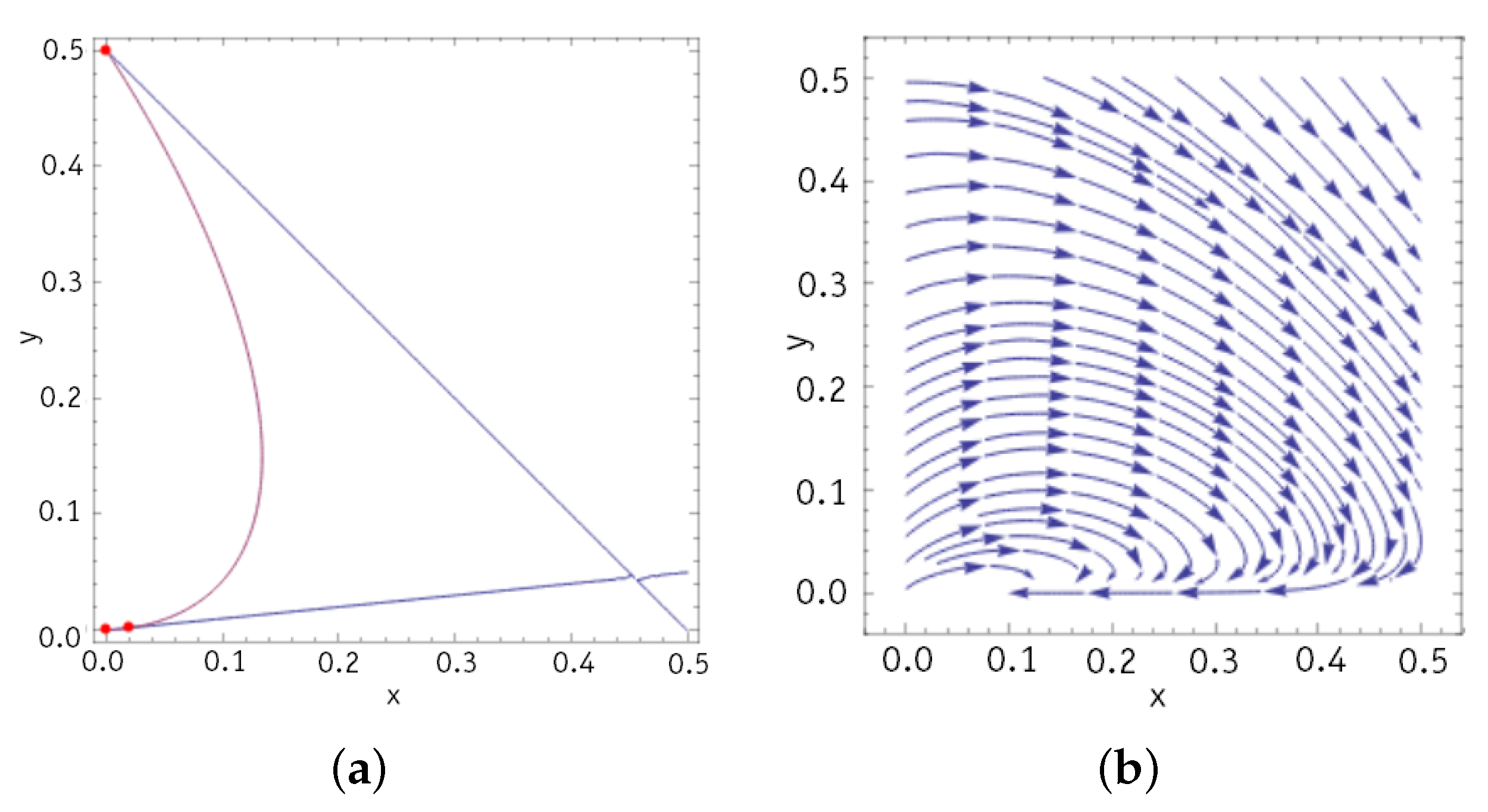
where possibly $ϵ=ϵ(x,y)$ depends continuously on $(x,y)$. Note that a similar rational term also occurs if infectives are isolated in a perfectly quarantine [14] ([p. 381]). The effect of this modification is that the nullcline of $\dot{y}$, beneath $y=0$ given before by the line $\beta (1-x-y)=\alpha +\delta$, changes to a curve through the origin, see Figure 2, which opens up the possibility that points in the interior are attracted by the DFE.

Figure 2. (a) Nullclines of $\dot{x}$ and $\dot{y}$ in (11) in blue, and nullcline of $\dot{y}$ in (14) in purple for parameters $\alpha =1$, $\beta =2$, $\gamma =0.1$, $\delta =0$, $ϵ=21/22$, $l=1$. The red dots show the intersection points between the nullclines. (b) For the same parameters some integral curves of (14), indicating the dynamics of the system.

Note that a multiplication of $ϵ\frac{x^{l}y}{{(x+y)}^l}$ by a smooth cut-off function $g\left(y\right)$ with $g\left(0\right)=1$ and $g\left(y\right)=0$ for $y>\eta$ with $\eta >0$ arbitrarily small does not change the behaviour of (14) near the line $y=0$, but leads to a system arbitrary near to (11) w.r.t. $C^0$-topology. Thus, it is sufficient to prove that the system (14) behaves near $(0,0)$ as claimed.

Remark 1.

Of course, there are various other terms which allow to modify (11) resp. (12) as claimed, and being near to these systems w.r.t. to $C^0$-topology. Yet, it does not seem to be easy to explicitly write down such systems and prove the required properties.

In the following, for constants ${ϵ}_0,{ϵ}_1\in \mathbb{R}$ we consider system (14) in the particular case where

$$ϵ=ϵ(x,y):={(1+\frac{\gamma }{\alpha })}^l\left({ϵ}_0+\beta {ϵ}_1(\gamma x-\alpha y)\right)$$

(15)

depends linearly on $(x,y)$ and is equal to ${(1+\frac{\gamma }{\alpha })}^l{ϵ}_0$ along the nullcline of $\dot{x}$. In this case, beneath the DFE $(0,0)$ the system (14) has for $\beta >\alpha +\delta$ and ${ϵ}_0<\beta -\alpha -\delta$ exactly one other equilibrium in the simplex, because $\dot{x}=0$ is equivalent to $y=\frac{\gamma }{\alpha }x$, i.e., $x+y=(1+\frac{\gamma }{\alpha })x$, and thus for $x\ne 0$ additionally the equation $\dot{y}=0$ holds if $(\beta -\alpha -\delta ){(x+y)}^l-\beta {(x+y)}^{l+1}-{(1+\frac{\gamma }{\alpha })}^l{ϵ}_0{x}^l=0$ or equivalently $(\beta -\alpha -\delta )-\beta (1+\frac{\gamma }{\alpha })x-{ϵ}_0=0$ is valid. Therefore, beneath the DFE the system (14) has the EE

$$(x_{EE},y_{EE}):=\frac{\beta -\alpha -\delta -{ϵ}_0}{\beta (1+\frac{\gamma }{\alpha })}(1,\frac{\gamma }{\alpha })$$

(16)

as only other equilibrium for $\beta >\alpha +\delta$ and ${ϵ}_0<\beta -\alpha -\delta$. This equilibrium EE is locally asymptotically stable for $\alpha >0$, $\beta >\alpha +\delta$, $\gamma >0$, ${ϵ}_0<\beta -\alpha -\delta$ and

$${ϵ}_0(l+1)+{ϵ}_1\alpha (\beta -\alpha -\delta -{ϵ}_0)<\beta -\delta +\gamma ,$$

(17)

because the Jacobian $D\widehat{f}(x_{EE},y_{EE})$ of the right hand side $\widehat{f}(x,y)$ of (14) at the EE is given by

$$\begin{array}{c}\hfill \left(\begin{array}{cc}-\gamma & \alpha \\ -\beta \frac{\gamma }{\alpha }{x}_{EE}-{ϵ}_0\frac{l{\gamma }^2}{{\alpha }^2(1+\frac{\gamma }{\alpha })}-{ϵ}_1\beta \gamma \frac{\gamma }{\alpha }{x}_{EE}& \beta -\alpha -\delta -\beta x_{EE}-2\beta \frac{\gamma }{\alpha }{x}_{EE}+{ϵ}_0\frac{-\alpha +(l-1)\gamma }{\alpha (1+\frac{\gamma }{\alpha })}+{ϵ}_1\beta \gamma x_{EE}\end{array}\right),\end{array}$$

(18)

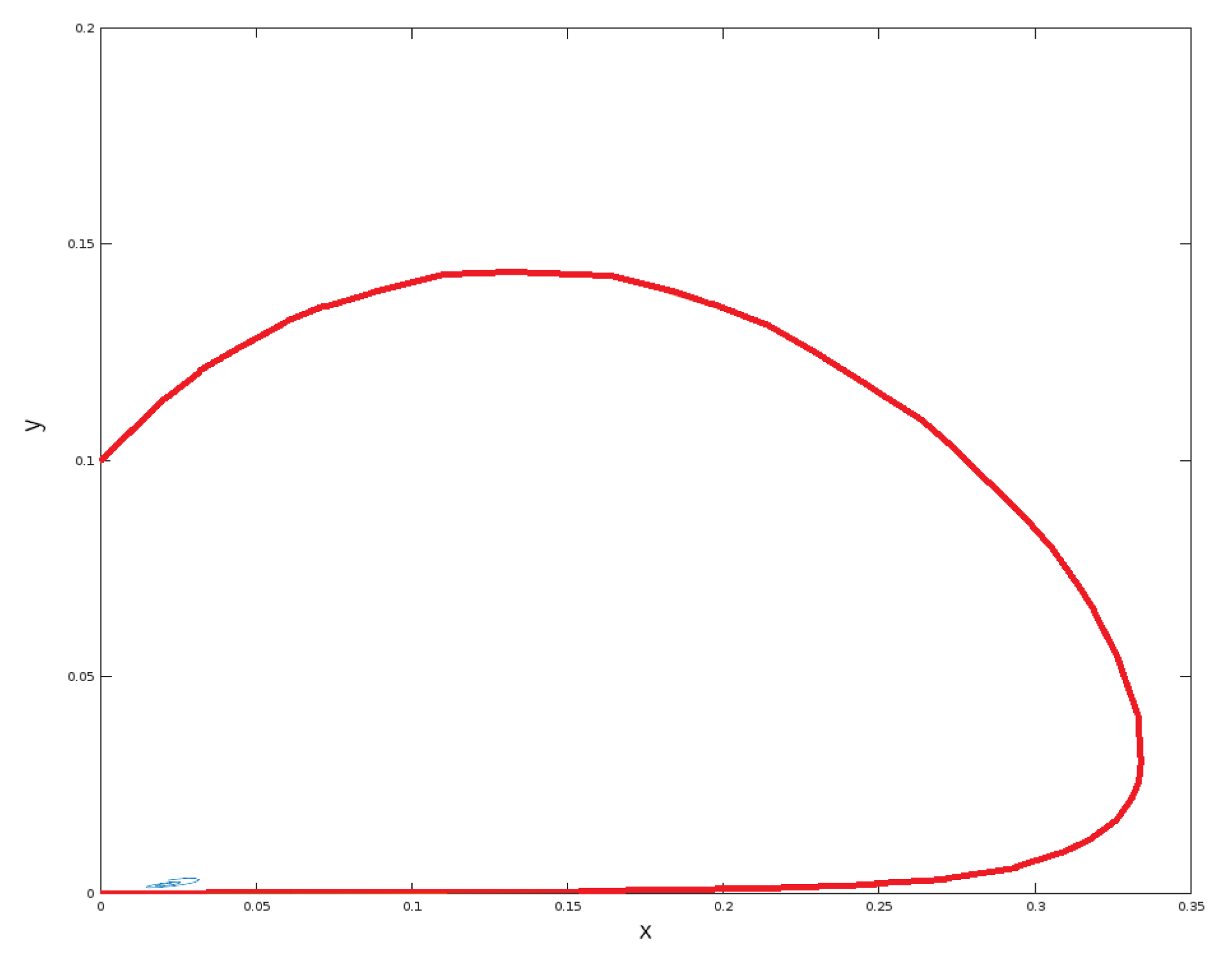
and this matrix has a positive determinant under the condition ${ϵ}_0<\beta -\alpha -\delta$ already required above for existence of the EE, and a negative trace if ${ϵ}_0(l+1)+{ϵ}_1\alpha (\beta -\alpha -\delta -{ϵ}_0)<\beta -\delta +\gamma$. Note that this condition does not only restrict the constants ${ϵ}_0,{ϵ}_1$, but also the exponent l. The following Lemma allows to conclude that in system (14) not only the EE can be locally attractive, but simultaneously also the DFE can attract interior points, see Figure 3 for a numerical example.

Figure 3. For the same parameters as in Figure 2 two solution curves of (14) with $ϵ=ϵ(x,y)$ given by (15) with ${ϵ}_0$: = $21/22$, the red one tends to the disease-free equilibrium and approximately separates the two basins of attraction, while the blue one first is nearly identical with the red one, but finally tends to the endemic equilibrium on the left below.

Lemma 1.

If $\alpha >0$, $\beta >\alpha +\delta$, $\gamma >0$, and $ϵ=ϵ(x,y)$ is given by (15) with ${ϵ}_0<\beta -\alpha -\delta$, then the DFE $(0,0)$ of system (14) attracts a subset of ${\widehat{{\Sigma }}}^2$ with non-empty interior, if additionally $\beta -\alpha -\delta +\gamma <{(1+\frac{\gamma }{\alpha })}^l{ϵ}_0$ holds, and such ${ϵ}_0$ exist if $1+\frac{\gamma }{\beta -\alpha -\delta }<{(1+\frac{\gamma }{\alpha })}^l$.

Proof. 

Using polar coordinates w.r.t. the 1-norm on the simplex ${\widehat{{\Sigma }}}_2$, i.e. $x=r(1-\varphi )$, $y=r\varphi$ for $r>0$, $0<\varphi <1$, with the generalized cosine and sine functions given by $C_{\infty }\left(\varphi \right)=1-\varphi$, $S_{\infty }\left(\varphi \right)=\varphi$ for $0<\varphi <1$ discussed, e.g., in [15], we obtain due to $r=x+y$, $\varphi =\frac{y}{x+y}$ and $dx=(1-\varphi )dr-rd\varphi$, $dy=\varphi dr+rd\varphi$, i.e., $dr=dx+dy$, $d\varphi =\frac{1}{r}((1-\varphi )dy-\varphi dx)$, the equations

$$\begin{array}{cc}\hfill \dot{r}& =r\left(\beta (1-r)\varphi -\gamma (1-\varphi )-\delta \varphi -ϵ{(1-\varphi )}^l\varphi \right)\hfill \\ \hfill \dot{\varphi }& =\varphi \left((1-\varphi )(\beta -\alpha -\delta -\beta r(1-\varphi )-\beta r\varphi -ϵ{(1-\varphi )}^l+\gamma )-\alpha \varphi \right)\hfill \end{array}$$

(19)

with $ϵ=ϵ(r,\varphi )={(1+\frac{\gamma }{\alpha })}^l\left({ϵ}_0+\beta {ϵ}_1(\gamma r(1-\varphi )-\alpha r\varphi )\right)$. Thus, if both r and $\varphi$ are small, then in the first equation the negative term $-\gamma (1-\varphi )$ dominates the bracket. To obtain a similar result for the second equation, we need $\beta -\alpha -\delta +\gamma <{(1+\frac{\gamma }{\alpha })}^l{ϵ}_0$, as then the term $\beta -\alpha -\delta -ϵ{(1-\varphi )}^l+\gamma$ dominating the bracket for small r and $\varphi$ is negative. Therefore, for such ${ϵ}_0$, the DFE attracts in the original system with coordinates $(x,y)$ a subset with non-empty interior near the origin between the line $y=0$ and the nullcline $\beta -\alpha -\delta -\beta x-\beta y-ϵ(x,y)\frac{x}{{(x+y)}^l}=0$ of $\dot{y}$. However, such ${ϵ}_0$ exist if $1+\frac{\gamma }{\beta -\alpha -\delta }<{(1+\frac{\gamma }{\alpha })}^l$. □

Particularly, note that for $\beta$ near to $\alpha +\delta$, i.e., shortly after the bifurcation discussed in Section 4.1, there is no ${ϵ}_0$ satisfying all conditions of Lemma 1, and even for $\beta$ so large that the conditions of Lemma 1 are satisfied, additionally condition (17) has to be satisfied to guarantee that both DFE and EE attract interior points of the simplex. Nonetheless, following Remark 1 other terms with a similar behaviour of the nullclines and not destroying local asymptotic stability of EE can be used, therefore we claim the validity of the following Theorem.

Theorem 4.

For $\alpha >0$, $\beta >\alpha +\delta$, $\gamma >0$, there exist ODE systems with continuous r.h.s. sufficiently near to (11) resp. (12) w.r.t. $C^0$-topology, which have two disjoint basins of attraction.

Moreover, as (11) resp. (12) are just normal forms, for nonlinear compartment models in arbitrary dimensions Theorem 4 implies the following Corollary.

Corollary 1.

For a smooth autonomous nonlinear compartment model $\dot{x}\left(t\right)=f(x\left(t\right),\lambda )$ satisfying (A1), (A2), and (A3) such that the DFE $(1,0,\cdots ,0)$ undergoes the generic bifurcation of codimension 2 described in Section 4.1 at a parameter $\lambda ={\lambda }_0$, where a locally asymptotically stable EE enters the simplex for sufficiently small $\lambda >{\lambda }_0$, there exists a continuous autonomous nonlinear compartment model nearby w.r.t. $C^0$-topology, where both DFE and EE have open basins of attraction for sufficiently small $\lambda >{\lambda }_0$.

4.3. Irreversible Rate-Induced Tipping for Time-Dependent Parameters in Idealized Systems, and Nearby Artifacts

To conclude that irreversible rate-induced tipping occurs in the idealized nonlinear compartment model (14) with time-dependent parameters, let us finally combine Lemma 1 with Theorem 1 about parameter paths, for which irreversible rate-induced tipping occurs for fast rates of parameter changes.

Corollary 2.

For the nonlinear compartment model (14) with $ϵ=ϵ(x,y)$ given by (15), there exist time-dependent parameters $\alpha \left(t\right)>0$, $\beta \left(t\right)>\alpha \left(t\right)+\delta$ and constant parameters $\gamma >0$, $\delta \ge 0$, ${ϵ}_0<\beta \left(t\right)-\alpha \left(t\right)-\delta$, ${ϵ}_1\in \mathbb{R}$ and $l>0$ satisfying $\beta \left(t\right)-\alpha \left(t\right)-\delta +\gamma <{(1+\frac{\gamma }{\alpha })}^l{ϵ}_0$ as well as (17), which give irreversible rate-induced tipping from the EE to the DFE.

Proof. 

By Lemma 1, the system (14) with frozen parameters in the specified parameter region has two disjoint basins of attraction, one attracted by the so-called endemic equilibrium EE and one attracted by the so-called disease-free equilibrium DFE. Now, on a time-dependent parameter change $\alpha \left(t\right),\beta \left(t\right)$, the coordinates (16) of the locally asymptotically stable equilibrium EE in the frozen system move, and by Theorem 1 there exists a parameter change with a rate so fast that the actual state of the non-autonomous system (14) leaves the basin of attraction of the EE and enters the basin of attraction of the DFE. Thus, there exist time-dependent parameters $\alpha \left(t\right),\beta \left(t\right)$ such that irreversible rate-induced tipping occurs in (14). □

Corollary 2 can be applied to conclude that not only the measures untertaken to contain a pandemic disease, but also the rate by which these measures are implemented may have a drastic influence on the success of a containment strategy [9]. Moreover, the non-idealized systems (11) resp. (12), which have an asymptotically stable equilibrium EE attracting all points in the interior of the simplex and a hyperbolic equilibrium DFE at a corner attracting only points on the boundary, are $C^0$-near to an idealized system by Theorem 4. Thus, for a fast parameter change in the non-idealized systems (11) resp. (12), there are trajectories which for a long time stay near to corresponding trajectories in the non-autonomous idealized system showing tipping. These trajectories can be considered as artifacts of rate-induced tipping, as they start near the EE, yet do not directly approach the EE, but tend for some time to the DFE. However, in contrast to the idealized system, after some time they again approach the EE in the non-idealized systems (11) resp. (12). Loosely speaking, in epidemology such an artifact may be interpreted as avoiding a pandemic wave through quickly implemented containment measures.

5. Conclusions

In this article, we have explained how irreversible rate-induced tipping can occur in nonlinear compartment models with time-dependent parameters, even if nearby systems have only one equilibrium attracting all interior points. The systems arising from a nonlinear compartment model after a generic bifurcation of codimension 2 at an equilibrium on a corner of the simplex can be modified to a $C^0$-near system with a continuous but non-smooth vector field near the corner, and such an idealized system has for frozen parameters two disjoint basins of attraction so that it allows irreversible rate-induced tipping for time-dependent parameters changing with a fast rate. Moreover, artifacts of irreversible rate-induced tipping in such an idealized system may be observed in the original system. Yet, we did not discuss how to calculate the rate at which parameters have to be changed so that rate-induced tipping occurs in idealized system resp. artifacts of tipping can be seen in the original nonlinear compartment models. A numerical calculation of such critical rates for a similar, but not identical system can be found in [9]. Further, some details seem to be open questions, e.g., to provide an explicit modifying term, which can be used directly after the bifurcation of the DFE occurred at $\beta =\alpha +\delta$. At least numerically there seems to be evidence for the existence of two basins of attraction in this case, but whether this really holds analytically remains open in this article.