Effective Pedagogy of Guiding Undergraduate Engineering Students Solving First-Order Ordinary Differential Equations

Abstract

An alternative pedagogical design is discussed that aims to guide engineering students to solve first-order ordinary differential equations (ODEs), and is based on students’ learning weaknesses identified from previous teaching and learning activities. This approach supported student’s self-enrichment through exploration of relevant resources in ODEs, and guided students towards the choice of their own effective ways for solving ODEs for different problems. This paper presents the practices on designing and delivering solution techniques for first-order linear ODEs using this approach for more than 400 undergraduate engineering students at a regional university in Australia during 2014–2017. The timeline involved initial experimentation in 2014 and 2015, followed by refinements to the pedagogy based on student’s feedback. The refined pedagogy was then used for the advanced mathematics course in 2016 and 2017. Significant improvements were made in student’s learning outcomes in effectively and accurately solving the first-order linear ODEs over this period.

1. Introduction

In undergraduate programs involving science and engineering, solving ordinary differential equations (ODEs) is an important part in designing and conducting scientific or engineering modelling [1,2,3,4]. In many Australian institutions, the fundamentals of different types of ODEs and the techniques to solve various ODEs are usually introduced immediately after the completion of elementary calculus [5]. On the other hand, in some universities in North America, ODEs are taught after the completion of a multivariable calculus course [6]. Hence, the students in different countries can experience different learning sequences to some extent, which is reflected in the textbooks adopted in universities in different regions [6,7,8,9,10]. Occasionally, some engineering mathematics textbooks popular in some US universities are adopted by a few Australian universities for advanced mathematics and engineering modelling [5,6] and the learning sequence therein may cause challenges in translating to different environment and educational systems.

In the current technology-enabled learning environment, students have opportunities to become more open leaners by finding information on almost every topic of mathematics from various sources, including the world-wide-web. As an addition to the traditional teaching and learning paradigms, this active learning enriches the process of knowledge building for many well-prepared self-learners. However, this also can confuse other students in terms of understanding a discourse that is built on some particular prerequisite knowledge of which they are lacking. Such confusion could be revealed when a student asked the teacher for clarifying his/her confusion, or when the teacher saw the work of a student in the submitted assignment. A teacher could help students to clarify the confusions individually upon knowing the problem. However, for those silent students who were more or less in a similar situation, they may still carry the confusion with them for a long time or forever. Such cases are common in advanced mathematics courses, for example, solving ODEs being a typical area of confusion [5,11,12,13].

Lozada et al. [14] recently presented a systematic review of classroom methodologies for teaching and learning ODEs based on a broad bibliometric analysis. Some scholars argued that the traditional teaching and learning methods focusing on applying algebraic procedures to solve ODEs may limit student’s learning [11,12,15]. However, studies on using other teaching and learning methods, such as qualitative learning, active learning, modelling based learning, problem-based learning, technology-based learning and so forth [2,16,17,18,19], may have addressed some issues in teaching and learning ODEs, but also raised more questions in the meantime. Hence, Lozada et al. suggested that teachers of ODEs should be encouraged to explore and enrich classroom activities with different methods to support students learning ODEs [14].

To facilitate effective learning of ODEs for the Australian students engaging in undergraduate engineering studies, a new approach was introduced to teach the advanced mathematics course for the students at a regional university in Australia from 2014. The new approach that incorporated the vertical knowledge progression with the lateral enrichment in mathematics based on the current prerequisite knowledge that students possessed was introduced to teaching ODEs and modelling for the engineering students. This approach not only supported student’s self-enrichment through exploring relevant resources in ODEs, but also guided students towards the choice of own effective ways for solving the ODEs for different problems. Through analyzing the common mistakes students made in solving the ODEs in their previous assignments, the causes of these problems were rooted, and alternatively more effective ways were explained and recommended to the students so as to clarify potential confusions on understanding different methods for solving the ODEs. This paper presents the practices on designing and delivering solving the first-order linear ODEs using this approach in recent years for the engineering students because the first-order linear ODEs is both the beginning level of differential equations and a pathway to solve ODEs numerically or some special ODEs like the Bernoulli equations [6,10,20,21,22]. Student’s improvements in solving ODEs using this approach are also discussed.

This pedagogical case study is guided by a mixed research paradigm that combines the evidence-based design and action research [23,24,25]. Action research is considered to be based in practice and not separate from it. Due to one author of this paper also teaching ODEs to the advanced mathematics course with different cohorts of students over four years during 2014–2017, our research design for this work aligns with action research. The initial evidence was the student’s performance data in solving the first-order linear ODEs in the same course offered in 2013 when different pedagogy and textbook were adopted by a different instructor. Our research question for this case study is whether the proposed pedagogy and subsequent refinement has brought significant and consistent improvement in students’ learning outcomes in solving the first-order linear ODEs technically. This question has been positively answered by the strong evidence of student’s performances in solving the first-order linear ODEs experimented using this pedagogy over four years during 2014–2017.

Section 2 presents the background information on how the new pedagogy was initiated through observing the student’s performance on solving the first-order linear ODEs in the previous offering delivered by a former lecturer. To address the issues identified in Section 2, alternative approaches to solve the ODEs are derived and recommended in Section 3. Section 4 presents the results of the two trials on using this approach for engineering students in 2014 and 2015, respectively. Section 5 describes the continuing effort on refining the pedagogy based on the student feedback in 2014 and 2015, and the analysis of student’s improvements in their learning outcomes using the refined pedagogy in 2016 and 2017, respectively. Further discussion on sustaining the successful teaching practices and learning outcomes with the pedagogy and concluding remarks are made in Section 6.

2. Background

In 2013, a popular advanced engineering mathematics textbook [6] was chosen as the prescribed textbook for the advanced mathematics course at the reginal university in Australia under this study. Unlike many other textbooks in which solving the first-order linear ODEs is progressed from solving the homogeneous linear ODEs by separation of variables to solving the inhomogeneous ODEs by integrating factors through elementary calculus, this textbook introduces integrating factors from solving the exact ODEs through multivariable calculus first. Its general procedure can be briefly summarized with a first-order ODE in the differential form as follows:

$$M(x,y)dx+N(x,y)dy=0.$$

(1)

Suppose there exists an implicit function u(x, y) = c (constant), and M(x, y) and N(x, y) can be associated with u(x, y) = c by

$$\frac{\partial u}{\partial x}=M \mathrm{and} \frac{\partial u}{\partial y}=N.$$

(2)

Equation (1) becomes the total differential of u(x, y) = c,

$$du=\frac{\partial u}{\partial x}dx+\frac{\partial u}{\partial y}dy=d[c]=0\stackrel{}{\to }Mdx+Ndy=0.$$

(3)

If u(x, y) = c has well-defined partial derivatives (first-order and mixed second-order), and its second-order partial derivatives are continuous, then the two mixed second-order derivatives of u(x, y) must be equal to each other, i.e.,

$$\frac{\partial M}{\partial y}=\frac{{\partial }^{2}u}{\partial y\partial x}=\frac{{\partial }^{2}u}{\partial x\partial y}=\frac{\partial N}{\partial x}\stackrel{}{\to }\frac{\partial M}{\partial y}=\frac{\partial N}{\partial x}.$$

(4)

In other words, if condition (4) is met, the solution u(x, y) = c to Equation (1) can be found by integrating any of the two partial derivatives in Equation (2), i.e.,

$$u(x,y)=c={\displaystyle \int Mdx}+g(y) \mathrm{or} u(x,y)=c={\displaystyle \int Ndy}+f(x),$$

(5)

where f(x) or g(y) is an unknown function involving x or y, respectively, which can be determined using Equation (2) again later.

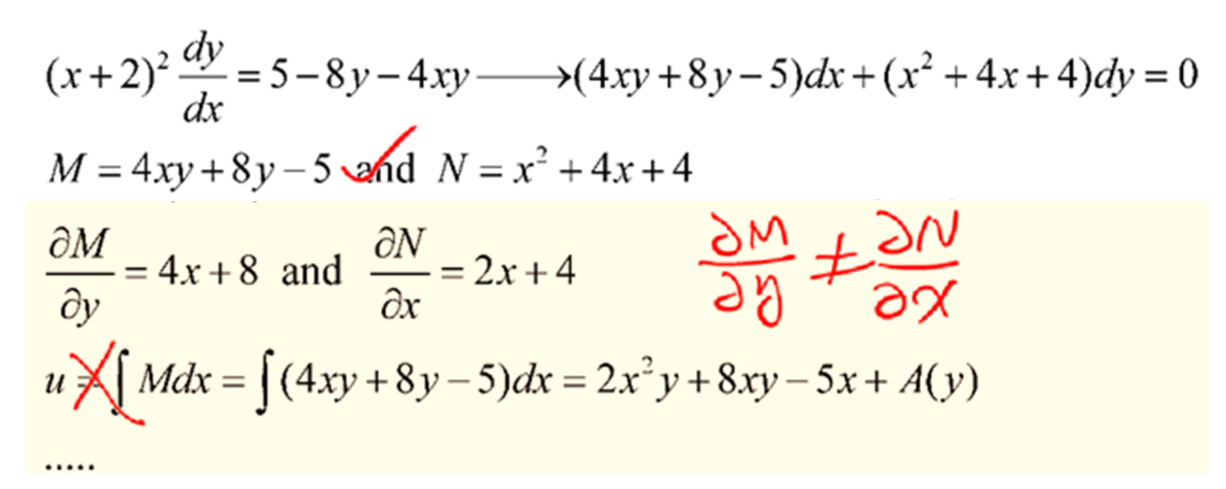
The following example is largely adopted from the textbook [6]. It assumed that students had completed a multivariable calculus course already, so some steps in the work were omitted in the book.

Example 1. 

Find the general solution to $\cos (x+y)dx+(3y^2+2y+\cos (x+y))dy=0$.

This first-order ODE is with

$$M=\cos (x+y), \mathrm{and} N=3y^2+2y+\cos (x+y).$$

Thus,

$$\frac{\partial M}{\partial y}=-\sin (x+y), \mathrm{and} \frac{\partial N}{\partial x}=-\sin (x+y).$$

Hence, this is an exact ODE and its general solution can be found by any integral in Formula (5) as follows.

$$u(x,y)={\displaystyle \int Mdx}={\displaystyle \int \cos (x+y)dx}=\sin (x+y)+g(y).$$

To find g(y), we differentiate this formula with respect to y and use Formula (4), obtaining

$$\frac{\partial u}{\partial y}=\cos (x+y)+\frac{dg}{dy}=N=3y^2+2y+\cos (x+y).$$

Hence,$\frac{dg}{dy}=3y^2+2y$. By integration,$g(y)=y^3+y^2+c_1$. Inserting this result into u(x, y) and observing u(x, y) = c in Formula (5), we obtain the answer

$$u(x,y)=\sin (x+y)+y^3+y^2=c.$$

In terms of solving this first-order ODE, the above solution is correct. However, this logical procedure does not seem so simple for students who do not have knowledge of multivariable calculus. When extending this procedure to solve a general ODE, the whole process of transforming the general ODE to an exact ODE so as to solve it is even more difficult for the students to understand, detailed as follows.

If the first-order ODE does not meet the condition in the Equation (4), i.e., for

$$P(x,y)dx+Q(x,y)dy=0$$

(6)

that does not produce $\frac{\partial P}{\partial y}=\frac{\partial Q}{\partial x}$, it may be possible to transfer the ODE (6) to an exact ODE like Equation (1) by multiplying a common function F(x, y), called an integrating factor, to both sides of Equation (6). Since the right side is zero, this multiplication effectively transfers Equation (6) to

$$FPdx+FQdy=0.$$

(7)

If both FP and FQ meet condition (4), i.e.,

$$\frac{\partial (FP)}{\partial y}=\frac{\partial (FQ)}{\partial x},$$

(8)

the similar process for an exact ODE can be applied to FP (as the new M = FP) and FQ (as the new N = FQ) to obtain a solution like

$$u(x,y)=c={\displaystyle \int FPdx}+g(y) \mathrm{or} u(x,y)=c={\displaystyle \int FQdy}+f(x).$$

(9)

Especially, if the integrating factor is only about x as F(x), Equation (8) becomes

$$F\frac{\partial P}{\partial y}=Q\frac{dF}{dx}+F\frac{\partial Q}{\partial x}\stackrel{}{\to }Q\frac{dF}{dx}=F(\frac{\partial P}{\partial y}-\frac{\partial Q}{\partial x})\stackrel{}{\to }\frac{1}{F}\frac{dF}{dx}=\frac{1}{Q}(\frac{\partial P}{\partial y}-\frac{\partial Q}{\partial x}).$$

Let

$$R=\frac{1}{Q}(\frac{\partial P}{\partial y}-\frac{\partial Q}{\partial x}).$$

(10)

The integrating factor F(x) can be found by

$$F(x)=e^{{\displaystyle \int R(x)dx}}.$$

(11)

The rest would be similar to that as obtaining the solution u(x, y) = c by FP = M and FQ = N as an exact ODE. This process is demonstrated with the following example that was a question in the assignment for the students at that time in 2013.

Example 2. 

Find the general solution to ${(x+2)}^2\frac{dy}{dx}=5-8y-4xy$.

This first-order ODE can be reorganized to its differential form,

$$(4xy+8y-5)dx+{(x+2)}^{2}dy=0,$$

where

$$P=4xy+8y-5=4y(x+2)-5, \mathrm{and} Q={(x+2)}^2.$$

By Equation (4),

$$\frac{\partial P}{\partial y}=4(x+2)\ne 2(x+2)=\frac{\partial Q}{\partial x}.$$

Hence, an integrating factor can be found using Equations (10) and (11) as follows.

$$\begin{array}{l}R=\frac{1}{Q}(\frac{\partial P}{\partial y}-\frac{\partial Q}{\partial x})=\frac{1}{{(x+2)}^2}[4(x+2)-2(x+2)]=\frac{2}{x+2}\\ F(x)=e^{{\displaystyle \int R(x)dx}}=e^{{\displaystyle \int \frac{2}{x+2}dx}}=e^{2\ln (x+2)}={(x+2)}^2.\end{array}$$

The solution can be found by

$$\begin{array}{l}u(x,y)={\displaystyle \int FPdx}={\displaystyle \int {(x+2)}^2[4y(x+2)-5]dx}={\displaystyle \int [4y{(x+2)}^3-5{(x+2)}^2]dx}\\ ={(x+2)}^{4}y-\frac{5}{3}{(x+2)}^3+g(y)\\ FQ=\frac{\partial u}{\partial y}={(x+2)}^4+g^{\prime }(y), \mathrm{and} FQ={(x+2)}^4\\ {(x+2)}^4+g^{\prime }(y)={(x+2)}^4\underset{}{\to }{g}^{\prime }(y)=0\stackrel{}{\to }g(y)=c_2\\ u(x,y)=c_1={(x+2)}^{4}y-\frac{5}{3}{(x+2)}^3+c_2.\end{array}$$

Therefore, the final solution to this ODE is

$${(x+2)}^{4}y-\frac{5}{3}{(x+2)}^3=c (=c_1-c_2) \mathrm{or} y=\frac{5}{3(x+2)}+\frac{c}{{(x+2)}^4}.$$

This logical procedure to solve the assigned ODE proved too challenging to follow for the students who did not have knowledge of multivariable calculus at the time. For example, of the thirty-two students engaged in distance learning, four students attempted to solve this ODE using this approach. Only one student managed to come close to the correct solution, whereas other three failed to follow through the process by a long margin, an example being shown in Figure 1. The initial mistake was made where $u=\int Mdx$ should not be used if $\frac{\partial M}{\partial y}\ne \frac{\partial N}{\partial x}$. An integrating factor defined by Equations (10) and (11) must be found first when this condition is not met.

Fortunately, following the introduction of these two approaches based on multivariable calculus to solve the first-order ODEs, the textbook also presents an alternative approach similar (but not the same) to the traditional approach of the integrating factor for the standard first-order linear ODE (12):

$$y^{\prime }+P(x)y=Q(x) \mathrm{as}$$

(12)

$$\{\begin{array}{l}y=e^{-h}\left({\displaystyle \int e^{h}Q(x)dx}+c\right)=e^{-h}{\displaystyle \int e^{h}Q(x)dx}+c{e}^{-h}\\ h={\displaystyle \int P(x)dx}\end{array}.$$

(13)

It is interesting to note that only two out of the thirty-two students used solution set (13) to attempt the assigned ODE and both obtained a fully correct solution, as shown in Figure 2. The unpopularity of solution set (13) among the students might be caused by the student’s lack of confidence in using this formula influenced by the negative perception of the use of multivariable calculus earlier.

The remaining twenty-six students used different approaches from other sources to attempt the assigned ODE. Among them, twenty-two of them used one of the conversional methods of integrating factors presented in their previous textbook for elementary calculus [8], which was also adopted in other textbooks [7,9,26,27,28]:

$$\{\begin{array}{l}\mu (x)y={\displaystyle \int \mu (x)Q(x)dx}+c\\ \mu (x)=e^{{\displaystyle \int P(x)dx}}\end{array}.$$

(14)

The popularity of this split implicit method among the students was likely because most of these students could understand the process of solution set (14) based on their knowledge of elementary calculus. As a result, fifteen out of the twenty-two students were able to obtain the desired solution or with minor errors. A common error for several students was made when obtaining the explicit solution from μ(x)y as shown in Figure 3. For the two cases, the mistakes were made when moving ${(x+2)}^2$ from the left side of the equation to the right side, which should lead to $y=\frac{5{(x+2)}^3}{3{(x+2)}^4}+\frac{c}{3{(x+2)}^4}$, rather than $\frac{5{(x+2)}^3}{3{(x+2)}^4}+c,$ or $y=\frac{5}{3(x+2)}+\frac{c}{3{(x+2)}^4}$, rather than $\frac{5+c}{3(x+2)}$. Such errors could be avoided if an explicit solution set like the Equation (13) was provided with a better explanation of the process for students.

The thirty-two distance students were chosen for observation because their learning was more depending on a suitable textbook to guide their progress compared with students on-campus where they could get direct assistance in their studies from lecturers, tutors, and fellow students. The overall performance of these thirty-two students on the assigned question in Example 2 is summarized in

Table 1. Summary of the performance on solving Example 2 by distance students.

	Solution (9)	Solution (13)	Solution (14)	Other	(Sub)total
Incorrect	3	0	7	4	14 (44%) 1
Correct	1 [25%] 2	2 [100%]	15 [68%]	0 [0%]	18 (56%)
(Sub)total	4 (12.5%)	2 (6%)	22 (69%)	4 (12.5%)	32 (100%)

¹ (%)—overall percentage; ² [%]—percentage of correction for the method.

.

Nearly a half of the thirty-two students came up with a wrong solution to this question. In terms of percentage, the explicit solution (13) returned the perfect correction rate even though only two students used this method, followed by the split implicit solution (14) with a correction rate of 68%. The solution (9) based on multivariable calculus yielded a correction rate of 25%, whereas the four students who did not use any of the methods presented above got wrong results. The overall correction rate of 56% for the distance students was below the class overall correction rate of 61% on solving this ODE.

3. The Initial Pedagogy for Solving the First-Order Linear ODEs

Observations in Section 2 led to some logical considerations for improving the performance of solving the first-order linear ODEs for engineering students who only had knowledge of elementary calculus. Firstly, we saw value in encouraging students to use an explicit solution, similar to Equation (13), but based on an understandable derivation process by elementary calculus, to solve the standard first-order linear ODE (12). Secondly, a split explicit solution set using integrating factors, rather than the split implicit solution set (14), could be recommended to students to solve the standard first-order linear ODEs. Students should also be advised to avoid using the methods involving multivariables calculus of which they lack, and any other methods that they did not understand. Based on these thoughts, two preferred methods were recommended to engineering students in 2014 with a tailored textbook [10].

3.1. Method of Variation of Parameters

Variation of parameters, also called variation of constants, is a general method to solve the inhomogeneous linear ODE (12) [10,29]. It is extended from the solution to the homogenous linear ODE for the corresponding inhomogeneous ODE (12). For the standard first-order linear ODE (12), if Q(x) = 0, it becomes a homogenous first-order linear ODE,

$$y^{\prime }+P(x)y=0.$$

(15)

This homogenous ODE can be solved using separation of variables as follows:

$$\frac{dy}{dx}=-P(x)y\underset{}{\to }\frac{dy}{y}=-P(x)dx\stackrel{}{\to }{\displaystyle \int \frac{dy}{y}}={\displaystyle \int -P(x)dx}\stackrel{}{\to }\ln y={\displaystyle \int -P(x)dx}+c_1$$

Hence,

$$y=e^{{\displaystyle \int -P(x)dx+c_1}}=e^{c_1}{e}^{{\displaystyle \int -P(x)dx}}=c{e}^{{\displaystyle \int -P(x)dx}}.$$

(16)

This is the general solution to the homogenous linear ODE (15). It already contains one unknown constant c so there is no need to add any new unknown constant from integral ${\displaystyle \int -P(x)dx}$.

To find the general solution to the inhomogeneous ODE (12), we replace the constant c in the general solution (16) to the homogenous ODE (15) by an unknown function u(x), i.e., assuming

$$y=u(x)e^{{\displaystyle \int -P(x)dx}}$$

(17)

to be the solution to the inhomogeneous ODE (12). Apply the product rule of differentiation to Formula (17)

$$\begin{array}{l}\frac{dy}{dx}=\frac{d[u(x)]}{dx}{e}^{{\displaystyle \int -P(x)dx}}+u(x)\frac{d[e^{{\displaystyle \int -P(x)dx}}]}{dx}=u^{\prime }(x)e^{{\displaystyle \int -P(x)dx}}+u(x)e^{{\displaystyle \int -P(x)dx}}\frac{d[{\displaystyle \int -P(x)dx}]}{dx}\\ =u^{\prime }(x)e^{{\displaystyle \int -P(x)dx}}+u(x)e^{{\displaystyle \int -P(x)dx}}[-P(x)]=[u^{\prime }(x)-P(x)u(x)]e^{{\displaystyle \int -P(x)dx}}\end{array}$$

or

$$\frac{dy}{dx}=u^{\prime }(x)e^{{\displaystyle \int -P(x)dx}}-P(x)u(x)e^{{\displaystyle \int -P(x)dx}}$$

(18)

Substitute Formulas (17) and (18) into the ODE (12)

$$\begin{array}{l}{u}^{\prime }(x)e^{{\displaystyle \int -P(x)dx}}-P(x)u(x)e^{{\displaystyle \int -P(x)dx}}+P(x)u(x)e^{{\displaystyle \int -P(x)dx}}=Q(x)\\ u^{\prime }(x)e^{{\displaystyle \int -P(x)dx}}=Q(x)\stackrel{}{\to }{u}^{\prime }(x)=Q(x)e^{{\displaystyle \int P(x)dx}}\end{array}$$

and then integrate both sides

$$u(x)={\displaystyle \int Q(x)e^{{\displaystyle \int P(x)dx}}dx}+c.$$

(19)

Substitute Formula (19) into Formula (17) to obtain the general solution to the inhomogeneous ODE (12)

$$y=u(x)e^{{\displaystyle \int -P(x)dx}}=e^{{\displaystyle \int -P(x)dx}}[{\displaystyle \int Q(x)e^{{\displaystyle \int P(x)dx}}dx}+c].$$

(20)

This is a unified explicit solution to ODE (12). The advantage of variation of parameters is that students are able to understand the derivation process that only requires an understanding of the basic concepts of elementary calculus. The other good fact about this method is that it provides students with an explicit form of solution, by which one can directly find the solutions to some first-order inhomogeneous linear ODEs comprising of relatively simple P(x) and Q(x).

Example 3. 

Find the general solution to$\frac{dy}{dx}+\frac{1}{x}y=2x+1$by Formula (20).

This is a standard first-order ODE with$P(x)=\frac{1}{x} \mathrm{and} Q(x)=2x+1$, both relatively simple. Its general solution can be obtained using the explicit form (20).

$$\begin{array}{l}y=e^{{\displaystyle \int -P(x)dx}}[{\displaystyle \int Q(x)e^{{\displaystyle \int P(x)dx}}dx}+c]=e^{{\displaystyle \int -\frac{1}{x}dx}}[{\displaystyle \int (2x+1)e^{{\displaystyle \int \frac{1}{x}dx}}dx}+c]=\frac{1}{x}[{\displaystyle \int (2x+1)xdx}+c]\\ =\frac{1}{x}[{\displaystyle \int (2x^2+x)dx}+c]=\frac{1}{x}[\frac{2}{3}{x}^3+\frac{1}{2}{x}^2+c]=\frac{2}{3}{x}^2+\frac{1}{2}x+\frac{c}{x}.\end{array}$$

Example 4. 

Find the general solution to the ODE in Example 2 by the Formula (20).

We first convert this ODE to its corresponding standard first-order form as follows.

$$\begin{array}{l}{(x+2)}^2\frac{dy}{dx}=5-8y-4xy\stackrel{}{\to }{(x+2)}^2\frac{dy}{dx}=5-4(x+2)y\\ {(x+2)}^2\frac{dy}{dx}+4(x+2)y=5\stackrel{}{\to }\frac{dy}{dx}+\frac{4}{x+2}y=\frac{5}{{(x+2)}^2}\\ P(x)=\frac{4}{x+2},Q(x)=\frac{5}{{(x+2)}^2}=5{(x+2)}^{-2}.\end{array}$$

Its general solution can be obtained using the explicit form (20).

$$\begin{array}{l}y=e^{{\displaystyle \int -P(x)dx}}[{\displaystyle \int Q(x)e^{{\displaystyle \int P(x)dx}}dx}+c]=e^{{\displaystyle \int -\frac{4}{x+2}dx}}[{\displaystyle \int \frac{5}{{(x+2)}^2}{e}^{{\displaystyle \int \frac{4}{x+2}dx}}dx}+c]\\ =e^{-4\ln (x+2)}[{\displaystyle \int \frac{5}{{(x+2)}^2}{e}^{4\ln (x+2)}dx}+c]=\frac{1}{{(x+2)}^4}[{\displaystyle \int \frac{5}{{(x+2)}^2}\cdot {(x+2)}^{4}dx}+c]\\ =\frac{1}{{(x+2)}^4}[{\displaystyle \int 5{(x+2)}^{2}dx}+c]=\frac{1}{{(x+2)}^4}[\frac{5}{3}{(x+2)}^3+c]=\frac{5}{3(x+2)}+\frac{c}{{(x+2)}^4}.\end{array}$$

This is much simpler than the process of solving this ODE through the process based on multivariable calculus used in Example 2.

Example 5. 

Find the general solution to$\frac{dy}{dx}+\frac{1}{1-x^2}y=2(1-x)$in –1 < x < 1.

This is a standard first-order ODE with$P(x)=\frac{1}{1-x^2}$and$Q(x)=2(1-x)$. Its general solution can be directly obtained using the explicit form (20).

$$\begin{array}{l}y=e^{{\displaystyle \int -P(x)dx}}[{\displaystyle \int Q(x)e^{{\displaystyle \int P(x)dx}}dx}+c]=e^{{\displaystyle \int -\frac{1}{1-x^2}dx}}[{\displaystyle \int 2(1-x)e^{{\displaystyle \int \frac{1}{1-x^2}dx}}dx}+c]\\ =e^{-{\displaystyle \int \frac{1}{(1-x)(1+x)}dx}}[{\displaystyle \int 2(1-x)e^{{\displaystyle \int \frac{1}{(1-x)(1+x)}dx}}dx}+c]=e^{-{\displaystyle \int \frac{1}{2}[\frac{1}{1+x}+\frac{1}{1-x}]dx}}[{\displaystyle \int 2(1-x)e^{{\displaystyle \int \frac{1}{2}[\frac{1}{1+x}+\frac{1}{1-x}]dx}}dx}+c]\\ =e^{-\frac{1}{2}[\ln (1+x)-\ln (1-x)]}[{\displaystyle \int 2(1-x)e^{\frac{1}{2}[\ln (1+x)-\ln (1-x)]}dx}+c]=e^{-\frac{1}{2}\ln \frac{1+x}{1-x}}[{\displaystyle \int 2(1-x)e^{\frac{1}{2}\ln \frac{1+x}{1-x}}dx}+c]\\ =e^{\ln \sqrt{\frac{1-x}{1+x}}}[{\displaystyle \int 2(1-x)e^{\ln \sqrt{\frac{1+x}{1-x}}}dx}+c]=\sqrt{\frac{1-x}{1+x}}[{\displaystyle \int 2(1-x)\sqrt{\frac{1+x}{1-x}}dx}+c]\\ =\sqrt{\frac{1-x}{1+x}}[{\displaystyle \int 2\sqrt{(1+x)(1-x)}dx}+c]=\sqrt{\frac{1-x}{1+x}}[{\displaystyle \int 2\sqrt{1-x^2}dx}+c]\\ {\displaystyle \int 2\sqrt{1-x^2}dx}={\displaystyle \int 2\sqrt{1-{\sin }^{2}t}\cos tdt}\underset{}{\overset{}{\leftarrow }}x=\sin t,t=\arcsin x,dx=\cos tdt\\ ={\displaystyle \int 2{\cos }^{2}tdt}=2{\displaystyle \int \frac{1+\cos 2t}{2}dt}=t+\frac{1}{2}\sin 2t=t+\sin t\cos t=\arcsin x+x\sqrt{1-x^2}\\ y=\sqrt{\frac{1-x}{1+x}}[{\displaystyle \int 2\sqrt{1-x^2}dx}+c]=\sqrt{\frac{1-x}{1+x}}[\arcsin x+x\sqrt{1-x^2}+c].\end{array}$$

This process is correct but it involves a lengthy procedure to get the solution. This is partly due to the complication of P(x) that is involved in two of the three integrals during the process. Logically, by the strategy of divide and conquer, it should be easier to deal with integrals involving complicated P(x) separately from the other integral involving Q(x). This brings an alternative approach, a new integrating factor, for solving the first-order ODE (12).

3.2. Integrating Factor by the Quotient Rule of Elementary Calculus

The standard first-order linear ODE (12) can be rewritten to its differential form (21),

$$dy+P(x)ydx=Q(x)dx.$$

(21)

Divide both sides of the above equation by a common function $\overline{\mu }(x)$

$$\frac{1}{\overline{\mu }(x)}dy+\frac{P(x)}{\overline{\mu }(x)}ydx=\frac{Q(x)}{\overline{\mu }(x)}dx$$

(22)

so that the left side becomes the differential of a quotient, i.e.,

$$d[\frac{y}{\overline{\mu }(x)}]=\frac{Q(x)}{\overline{\mu }(x)}dx.$$

(23)

Expand Equation (23) to the following form

$$\frac{\overline{\mu }(x)dy-{\overline{\mu }}^{\prime }(x)ydx}{{[\overline{\mu }(x)]}^2}=\frac{Q(x)}{\overline{\mu }(x)}dx$$

or

$$\frac{1}{\overline{\mu }(x)}dy-\frac{{\overline{\mu }}^{\prime }(x)}{{[\overline{\mu }(x)]}^2}ydx=\frac{Q(x)}{\overline{\mu }(x)}dx.$$

(24)

By comparing both sides of the Equations (22) and (24), both equations will be equivalent if the following condition is met

$$\frac{P(x)}{\overline{\mu }(x)}=-\frac{\overline{{\mu }^{\prime }}(x)}{{[\overline{\mu }(x)]}^2} \mathrm{or} \frac{{\overline{\mu }}^{\prime }(x)}{\overline{\mu }(x)}=-P(x).$$

(25)

The Equation (25) is equivalent to

$$d[\ln \overline{\mu }(x)]=-P(x)\stackrel{}{\to }\ln \overline{\mu }(x)=-{\displaystyle \int P(x)dx}.$$

This can be explicitly expressed as

$$\overline{\mu }(x)=e^{-{\displaystyle \int P(x)dx}}.$$

(26)

Therefore, if the common function, or the integrating factor $\overline{\mu }(x)$ is determined by Equation (26), the standard first-order ODE (12) can be transferred to Equation (23). Integrate both sides of Equation (23)

$$\frac{y}{\overline{\mu }(x)}={\displaystyle \int \frac{Q(x)}{\overline{\mu }(x)}dx}+c$$

or

$$\{\begin{array}{l}y=\overline{\mu }(x)[{\displaystyle \int \frac{Q(x)}{\overline{\mu }(x)}dx}+c]\\ \overline{\mu }(x)=e^{-{\displaystyle \int P(x)dx}}\end{array}.$$

(27)

Hence, the solution defined by equation set (27) produces a split explicit solution to the standard first-order linear ODE (12), by which the whole process is divided into two separate steps for a better control similar to solution set (14) that, however, produces an implicit solution.

Example 6. 

Find the general solution to the ODE in Example 4 by Formula (27).

The integrating factor involving$P(x)=\frac{4}{x+2}$can be determined by Formula (26) as follows.

$$\overline{\mu }(x)=e^{{\displaystyle \int -P(x)dx}}=e^{{\displaystyle \int -\frac{4}{x+2}dx}}=e^{-4\ln (x+2)}=\frac{1}{{(x+2)}^4}={(x+2)}^{-4}.$$

The explicit solution to the ODE can be obtained by the first equation in solution set (27) as

$$\begin{array}{l}y=\overline{\mu }(x)[{\displaystyle \int \frac{Q(x)}{\overline{\mu }(x)}dx}+c]=\frac{1}{{(x+2)}^4}[{\displaystyle \int \frac{5{(x+2)}^{-2}}{{(x+2)}^{-4}}dx}+c]=\frac{1}{{(x+2)}^4}[{\displaystyle \int 5{(x+2)}^{2}dx}+c]\\ =\frac{1}{{(x+2)}^4}[\frac{5}{3}{(x+2)}^3+c]=\frac{5}{3(x+2)}+\frac{c}{{(x+2)}^4}.\end{array}$$

This is the same as the solution obtained in Example 2 and in Example 4 by the unified explicit solution (20).

Example 7. 

Find the general solution to the ODE in Example 5 using solution set (27).

This is a standard first-order ODE with$P(x)=\frac{1}{1-x^2}$and$Q(x)=2(1-x)$. Its integrating factor can be determined using Formula (26).

$$\begin{array}{l}\overline{\mu }(x)=e^{{\displaystyle \int -P(x)dx}}=e^{{\displaystyle \int -\frac{1}{1-x^2}dx}}=e^{-{\displaystyle \int \frac{1}{(1-x)(1+x)}dx}}=e^{-{\displaystyle \int \frac{1}{2}[\frac{1}{1+x}+\frac{1}{1-x}]dx}}\\ =e^{-\frac{1}{2}[\ln (1+x)-\ln (1-x)]}=e^{-\frac{1}{2}\ln \frac{1+x}{1-x}}=e^{\frac{1}{2}\ln \frac{1-x}{1+x}}=e^{\ln \sqrt{\frac{1-x}{1+x}}}=\sqrt{\frac{1-x}{1+x}}.\end{array}$$

Its explicit solution can be obtained using Formula (27)

$$\begin{array}{l}y=\overline{\mu }(x)[{\displaystyle \int \frac{Q(x)}{\overline{\mu }(x)}dx}+c]=\sqrt{\frac{1-x}{1+x}}[{\displaystyle \int \frac{2(1-x)}{\sqrt{\frac{1-x}{1+x}}}dx}+c]=\sqrt{\frac{1-x}{1+x}}[{\displaystyle \int 2\sqrt{(1+x)(1-x)}dx}+c]\\ =\sqrt{\frac{1-x}{1+x}}[{\displaystyle \int 2\sqrt{1-x^2}dx}+c]=\sqrt{\frac{1-x}{1+x}}[\arcsin x+x\sqrt{1-x^2}+c].\end{array}$$

This is the same as the solution obtained in Example 5 by the unified explicit solution (20), but with a better control over the entire process. Note that this split method does not need further manipulation to obtain the explicit solution, unlike using the split implicit solution (14). Therefore, this solution is the other preferred approach recommended to the engineering students in 2014, in addition to the unified explicit solution (20).

4. The First Trials and Observations

In 2014, for the first time, after going through the derivation processes of these two methods for obtaining the explicit solutions to the first-order linear ODE (12), the engineering students in the advanced mathematics course were recommended to choose either of the two explicit methods to solve first-order linear ODEs. One question involving solving a first-order linear ODE was set as a part of an assignment. To promote collaborations between the distance and on-campus students, the assessment was set as a group assignment, and no more than five students could work together as a team. Thirty-eight submissions from 131 students were received. A brief summary of the team’s preferred method for solving the assigned ODE is shown in

Table 2. Summary of solving the first-order linear ODE in the assignment in 2014.

	Solution (20)	Solution (27)	Other	(Sub)Total
Incorrect	0	4	5	9 (24%) 1
Correct	3 [100%] 2	23 [85%]	3 [37.5%]	29 (76%)
(Sub)total	3 (8%)	27 (71%)	8 (21%)	38 (100%)

¹ (%)—overall percentage; ² [%]—percentage of correction for the method.

, along with the performance with a chosen method.

Although only three teams used the unified explicit form (20) to solve this ODE, all of them obtained the correct solution (Figure 4a). The split explicit form (27) was chosen by twenty-seven out of thirty-eight teams (or 71% of all teams) to solve this ODE with 23 teams out of the 27 reaching the correct solution (Figure 4b). The four teams out of the 27 that obtained wrong solutions were correct in the process of using solution (27), but made mistakes in integration (Figure 5). The core of the integration should be conducted by integration by parts as shown on the right side of the example.

Eight teams, mostly as individuals, chose a method similar to the split implicit solution (14) or different methods from other sources to solve this ODE, but only three out of the eight obtained the correct solution. The wrong solutions were due to either using an incorrect process or having made mistakes in the integral. Most students from these eight teams either missed or failed the same course in previous years, but still used the previous textbooks for this new offering. Most of them dropped out of this course eventually. Even including these eight teams, most teams (76% overall) obtained correct solutions, and this rate went up to 87% for the 30 teams who used either of the two explicit methods.

The encouraging outcome in 2014 inspired the second trial of guiding students solving the first-order linear ODEs using the same recommendations in 2015. This time, twenty-seven teams from 90 students submitted assignments, in which one question was on solving a first-order linear ODE. Like the 2014 offering, the brief summary of the team’s preferred method for solving this ODE is shown in

Table 3. Summary of solving the first-order linear ODE in the assignment in 2015.

	Solution (20)	Solution (27)	Other	(Sub)total
Incorrect	0	1	3	4 (15%) 1
Correct	4 [100%] 2	17 [94%]	2 [40%]	23 (85%)
(Sub)total	4 (15%)	18 (67%)	5 (18%)	27 (100%)

¹ (%)—overall percentage; ² [%]—percentage of correction for the method.

, along with the performance with a chosen method.

Similar patterns occurred again. The four teams who used the unified explicit form (20) to solve this ODE all came up with the correct solution. The seventeen submissions out of the 18 teams who used the split explicit form (27) to solve this ODE presented the correct solution. The other team was correct in the process of applying the split solution (27), but made mistakes in integration. The remaining five teams, mostly as individuals, chose a method similar to the split implicit solution (14) or different methods from other sources to solve this ODE, but only two of them obtained the correct solution.

Overall, twenty-three teams, or 85% of all teams, obtained correct solutions, dominated by those teams who used either of the two explicit solutions.

5. The Feedback, Refinement and Further Improvements

The new approach to guide students solving the first-order linear ODEs experimented in 2014 and 2015 brought significant improvements in effectively solving the related ODEs compared with the outcome in the previous year. This approach was well accepted by the engineering students in 2014 and 2015, as their preferred way to solve the first-order linear ODEs. Hence, the purpose of progressing the vertical knowledge building in solving the ODEs was largely realized. Meanwhile, in each offering in 2014 and 2015, several students privately asked some questions relevant to but beyond the two recommended explicit methods, due to a curiosity and/or some confusions. All the questions were answered privately to the individuals who were satisfied with the explanations. Those questions, though asked by only a small number of students, implied that there was a need to widen the scope of solving the first-order linear ODEs beyond the two recommended methods for the purpose of lateral enrichment and rationalization.

Hence, a special tutorial note was prepared as an optional learning activity for the engineering students in 2016 and 2017 [5], in addition to the two preferred explicit methods. This special tutorial note provided students with both the comprehensive procedures for each of the four commonly used methods (one implicit and three explicit approaches) in different sources to solve the first-order linear ODEs and the inter-convertibility among them so as to widen student’s understanding of these mostly related methods.

This refined pedagogy was introduced to the engineering students in 2016. Like previous offerings, there was one question involving solving a first-order linear ODE in the first assignment. Thirty-seven group submissions from 120 students were received. A brief summary of the team’s preferred method for solving the ODE is shown in

Table 4. Summary of solving the first-order linear ODE in the assignment in 2016.

	Solution (20)	Solution (27)	Other	(Sub)total
Incorrect	0	3	1	4 (11%) 1
Correct	2 [100%] 2	30 [91%]	1 [50%]	33 (89%)
(Sub)total	2 (5.5%)	33 (89%)	2 (5.5%)	37 (100%)

¹ (%)—overall percentage; ² [%]—percentage of correction for the method.

, along with the performance with the chosen method.

Only two teams used the unified explicit form (20) to solve this ODE and obtained the correct solution. Thirty-three teams (or 89% of all teams) used the split explicit form (27) to solve this ODE with 30 team reaching the correct solution. The three teams that obtained wrong solutions were correct in the process of using the split solution (27), but made mistakes in integration. Two other submissions by individuals used different methods to solve this ODE, and one obtained the correct solution.

Overall, thirty-three teams, or 89% of all teams, obtained the correct solution to the ODE, dominated by those teams who used either of the two explicit solutions.

The refined approach was used to guide the engineering students in 2017 again. To evaluate individual’s understanding of and effectiveness in solving the first-order linear ODEs, this time the assignment was set as individual assessment for 94 students. Like previous offerings, one question involving solving a first-order linear ODE was assigned to the students. A brief summary of the preferred method for solving the ODE by the 94 students is shown in

Table 5. Summary of solving the first-order linear ODE in the assignment in 2017.

	Solution (20)	Solution (27)	Other	(Sub)total
Incorrect	0	2	3	5 (5%) 1
Correct	0	89 [98%] 2	0 [0%]	89 (95%)
(Sub)total	0	91 (97%)	3 (3%)	94 (100%)

¹ (%)—overall percentage; ² [%]—percentage of correction for the method.

, along with the performance with the chosen method.

Surprisingly, the unified explicit form (20) was not chosen by any student. Instead, except three students, ninety-one students (or 97% of all students) preferred to solve this ODE using the split explicit form (27), among them eighty-nine (or 98% of this group) reaching the correct solution, including all 22 distance students. The three students who chose a different method from other sources to solve the ODE all came up with incorrect solutions. It seemed that not all students would pay attention to the teacher’s recommendation and extra explanations of different methods for solving the first-order linear ODEs.

6. Discussion and Concluding Remarks

The effort on the pedagogy that was more suitable and more effective for undergraduate engineering students at a regional university in Australia brought significant improvements in students’ learning outcomes in solving the first-order linear ODEs over four years during 2014–2017. This continued effort took different stages of progression over this time.

The pedagogical design was based on the learning weaknesses identified from previous teaching and learning activities and outcomes, which initiated the idea of guiding students solving the first-order linear ODEs by recommending two methods for obtaining the explicit solution directly to such ODEs. The realization of this pedagogical design was tested repeatedly in 2014 and 2015 to confirm the real impact on and significant improvement in students learning outcomes in effectively and accurately solving such ODEs. By responding to student’s feedback in these two trials, further refinement of this approach in terms of widening the scope of solving the first-order linear ODEs by other methods was added to the initial pedagogical design. This refinement provided students with a logical way of unifying the common methods for solving the first-order linear ODEs presented in different sources, which not only clarified confusions to some students, but also satisfied other students’ curiosities in various methods.

All these attempts had resulted in a steady and substantial increase in effectively and accurately solving the first-order linear ODEs over four years. Compared with the overall rate of about 60% in obtaining the correct solution to the assigned ODE by the students in the previous offering, this rate was lifted to 76%, 85%, 89% and 95% from 2014 to 2017 (Figure 6). It indicates that the new pedagogy of combining the vertical skills building with lateral knowledge enrichment was more effective and successful in improving student’s learning outcomes and experiences.

This study also suggests that student’s retention of the skills and knowledge gained in previous mathematics courses is vital for their smooth progression in advanced mathematics courses, the similar observations being made previously already [30,31]. For example, the incorrect solutions to Example 2 showed in Figure 3 indicate that students made mistakes in simple algebraic manipulations, which should not be a problem for any engineering students in their second-year study. From 2014 to 2017, every time one or more students could not handle integration correctly during solving the ODEs, as being shown Figure 5. Regardless of how much extra effort the educators can make to the pedagogy of the advanced mathematics courses, solving any ODEs requires skills and knowledge of integration and differentiation, irrelevant to whichever method of solving the ODE is chosen. Therefore, providing students with appropriate learning experiences in each of the courses in the mathematics curriculum, particularly the foundation courses, must be promoted and sustained during the entire study of any mathematics-heavy programs, such as undergraduate engineering programs.

Reaching a high level of teaching and learning satisfaction is difficult, and maintaining such a high level is even tougher. It requires an educator to willingly engage with student’s learning activities and respond to student’s feedback, to be experienced in quickly identifying the gaps in the curriculum and weaknesses commonly exhibited by students, to be knowledgeable about how to effectively fill the gaps or remedy the weaknesses, and to be passionate about student’s learning and positive progression. We encourage educators to explore innovative pedagogy to teach advanced mathematical topics like ODEs, and to enhance their own technical knowledge and skills in these advanced topics.

Our study also suggests the importance of flexible or informal approaches when students do not possess the necessary background whilst learning ODEs. This is the case where the method based on multivariable calculus was introduced. Making the extra learning material as an optional tutorial helps those keen students with curiosity on the method and derivation learn more, but does not add further pressure or confusion to other students who have no desire to learn the specific method and origin. We acknowledge that students may have different personal goals in different courses for their study.

No matter how much extra effort an educator can make to the pedagogy and curriculum, not all students would pay attention to or appreciate the teacher’s effort. As it has been widely reported, often some students enrolled in a course would not follow any instruction or would do nothing during the course [32,33,34]. Aiming to achieving a maximum rate of 100% from students would be an unrealistic task on most occasions, particularly involving advanced mathematics.

An adoption and adaption of this proposed pedagogy has the potential impact on assisting all undergraduate students starting the journey of learning differential equations for applications by easing the pressure of understanding the mathematical procedures and effectively utilizing the fundamental techniques to solve the first-order linear ODEs, which is the first step to the rest of the differential equations. However, we would also like to point out that this pedagogy is limited to solve the ODEs that can be converted to the first-order linear ODEs. For the first-order nonlinear ODEs that cannot be converted to the linear ODEs, some may be solved by the exact differential method based on multivariable calculus, such as Example 1, and many more can only be solved by numeric methods.

This pedagogical study was focused on guiding students to effectively solve the first-order linear ODEs technically, but did not look into how students would apply the technical skills for solving real problems or problems with real engineering implications. This would be another area worthy of further investigation in the near future.

We would also like to apply this mixed research paradigm combining the evidence-based design and the action research to other mathematics teaching and learning areas where multiple approaches are available to solve the same problem, with which students may feel confused by the selection of a more appropriate method from many options, such as numeric methods for solving ODEs, multiple approaches to deal with questions with complex numbers.