Adaptive Fault Estimation for Hyperbolic PDEs

Abstract

The new adaptive fault estimation scheme is proposed for a class of hyperbolic partial differential equations in this paper. The multiplicative actuator and sensor faults are considered. There are two cases that require special consideration: (1). only one type of fault (actuator or sensor) occurs; (2). two types of faults occurred simultaneously. To solve the problem of fault estimation, three challenges need to be solved: (1). No prior information of fault type is known; (2). Unknown faults are always coupled with state and input; (3). Only one boundary measurement is available. The original plant is converted to Observer canonical form. Two filters are proposed and novel adaptive laws are developed to estimate unknown fault parameters. With the help of the proposed update laws, the true state of the faulty plant can be estimated by the proposed observers composed of two filters. By selecting a suitable Lyapunov function, it is proved that under unknown external disturbance, the estimation errors of state parameters and fault parameters decay to arbitrarily small value. Finally, the validity of the proposed observer and adaptive laws is verified by numerical simulation.

1. Introduction

Process monitoring involving the fault detection and estimation is crucial to process safety. The existing technology can be divided into three categories: based on mathematical model, based on data-driven empirical model and fault detection technology combining empirical model and plant prior information. Data driven method can refer to system identification areas [1,2,3,4], etc. While the mathematical model method has better extrapolation, and empirical model is more convenient to design. Many works have made important contributions in the aspect of fault detection: see [5,6,7,8,9,10,11,12]. Those contributions contain adaptive observer [13,14], sliding mode observer [15]. The recent works [16,17] present full-order and reduced-order sliding mode observer (SMO) for Markov jump systems. In [18], the linear matrix inequality (LMI) theory is used to realize the fault estimation of synchronous actuator and sensor for Markov jump system. On this basis, the stochastic process model is established, the approximate fault estimation is made, and the time to failure (TTF) estimation is achieved in [19,20].

In practical application, robust fault estimation is the key to realize real-time monitoring, diagnosis and fault-tolerant control. Many contributions have been made to solve the related problems. In [21], the augmented system is first configured to contain the plant state of interest and the augmented state of the fault. An optimization method of unknown input observer (UIO) based on LMI is proposed to minimize the stability of the estimation error dynamic and the influence of disturbance. Aiming at the problem of state estimation and fault estimation for discrete time systems, in [22], a robust estimation method based on linear matrix inequality (LMI) technique and generalized systems theory is proposed. An observer design method is proposed in [23] for Takagi-Sugeno fuzzy systems in the presence of process uncertainties and unexpected failures. Concretely, a robust state estimation and fault estimation for all controlled objects are realized by using UIO technology, augmented system theory and sliding mode control method.

A lot of industrial systems, such as fluid flow and chemical reaction processes, all exhibit spatio-temporal dynamics, that is, the state of the system is spatial-varying and time-varying. Hence, the temporal dynamic representation is not suitable for displaying their behavior, and the observer design is a challenging problem. Moreover, the fault detection and estimation of space-time systems are more challenging. Most of the existing fault detection methods are based on modal analysis. For example, [24] uses the modal analysis technique based method to develop a fault detection observer. Similarly, the work [25] designs a robust observer to solve the problem of fault detection and state estimation.

The above techniques make use of the model approximation, which results in false alarm due to model reduction. In [26], an adaptive PDE observer is developed for positive system to realize fault accommodation. In our recent work [27], two filters are proposed based on the Luenberger observer, and then novel parameter adaptation laws were proposed to address boundary fault estimation issues.

In this paper, we propose a scheme for state and fault estimation of a linear hyperbolic PDE system with unknown disturbances based on the plant observer canonical form. Unlike [28], where additive faults are considered and some real positive conditions need to be satisfied, this article considers multiplicative faults. Especially, when the actuator and sensor fail at the same time, the estimation problem becomes more challenging.

The contributions are as follows:

• The problem of state and fault estimation in two cases is solved: (1). only one type of fault (sensor or actuator) occurs; (2). the sensor and actuator failed simultaneously.
• By proposing novel transformation, the observer canonical form of the system of interest is obtained. Consequently, two auxiliary filters are designed, and based on which the novel adaptation laws are proposed.
• We show that in sense of Lyapunov stability fault parameter estimation converges exponentially fast.

This paper is organized as follows: Section 2 introduces the system considered and multiplicative boundary faults. Section 3 describes the design of fault parameter adaptation law based on the observer canonical form. In Section 4, numerical simulations are performed to illustrate the validity of the proposed results.

Notation

Given the vector variables $v\left(\xi \right),\forall \xi \in [0,1]$ which is spatially varying and continuous, the following operator is defined:

$$H_{\beta }\left[v\left(\xi \right)\right]={\int }_0^1{e}^{\beta \xi }v\left(\xi \right)d\xi ,$$

(1)

where $\beta$ is a real number, with the derived norm

$${∥v∥}_{\beta }^2=H_{\beta }\left[v^{T}v\right]={\int }_0^1{e}^{\beta \xi }{v}^T\left(\xi \right)v\left(\xi \right)d\xi .$$

(2)

The integral operator (1) has the following property

$$2H_{\beta }\left[v{v}_{\xi }\right]=e^{\beta }{v}^2\left(1\right)-v^2\left(0\right)-\beta {∥v∥}_{\beta }^2,$$

(3)

where $v_{\xi }$ represents the derivative of $v\left(\xi \right)$ w.r.t the spatial variable $\xi$. In subsequent sections, we will write ${\partial }_{t}v(\xi ,t)$ (or $v_t(\xi ,t)$) and ${\partial }_{\xi }v(\xi ,t)$ (or $v_{\xi }(\xi ,t)$) to stand for $\frac{\partial v(\xi ,t)}{\partial t}$ and $\frac{\partial v(\xi ,t)}{\partial \xi }$, respectively.

The norm ${∥v∥}_{\beta }$ is equivalent to the standard $L_2$-norm, namely, there exist positive constants ${\kappa }_1$, ${\kappa }_2$ such that

$${\kappa }_1{∥v∥}_{\beta }\le {∥v∥}_0\le {\kappa }_2{∥v∥}_{\beta }.$$

(4)

For brevity, the argument in time and space are often omitted, i.e., $∥u∥=∥u\left(t\right)∥$, $v=v(\zeta ,t)$.

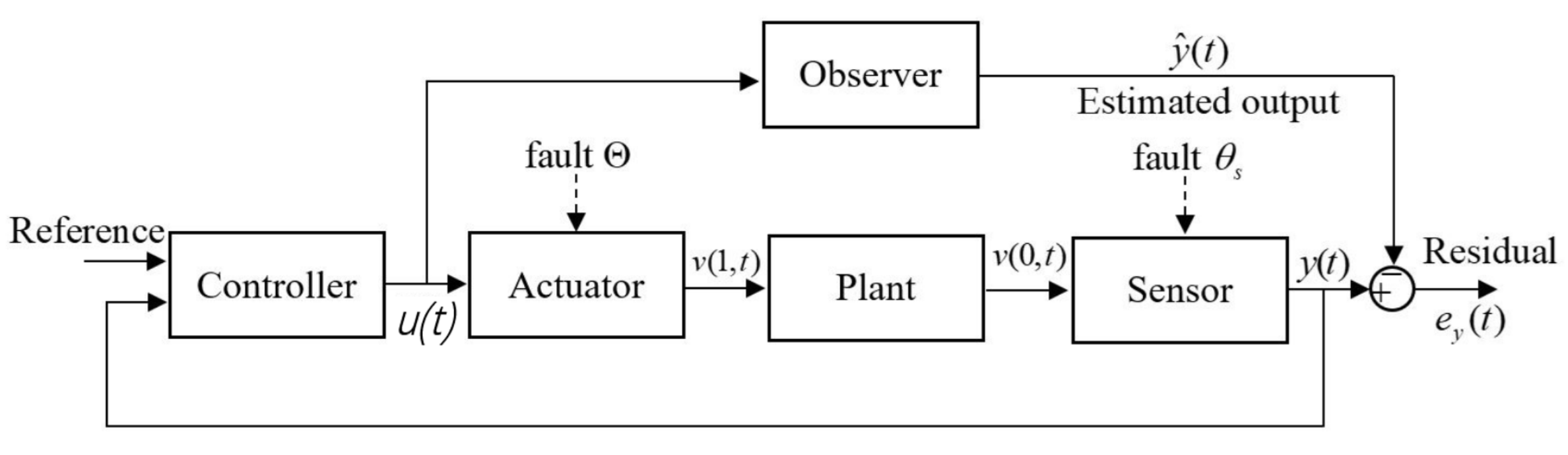
2. Problem Statement

We consider the following PDEs:

$$\begin{array}{c}{v}_t(\xi ,t)=v_{\xi }(\xi ,t)+g\left(\xi \right)v(0,t)+\varphi \left(t\right)\hfill \\ +{\int }_0^{\xi }f(\xi ,\zeta )v(\zeta ,t)d\zeta \hfill \\ +{\int }_{\xi }^{1}h(\xi ,\zeta )v(\zeta ,t)d\zeta ,\hfill \end{array}$$

(5)

$$\begin{array}{c}v(1,t)=u\left(t\right),\hfill \end{array}$$

(6)

$$\begin{array}{c}y\left(t\right)=v(0,t)\hfill \end{array}$$

(7)

defined on the domain $\left\{t\in {\mathbb{R}}^{+},\xi \in \left(0,1\right)\right\}$, where $g,f$ and h denote system coefficient functions, $v(\xi ,t)\in L^2(0,1)$, $\forall (\xi ,t)\in [0,1]\times {\mathbb{R}}^{+}$ stands for the system state, $L^2(0,1)$ denotes a real Hilbert space with the inner product $〈v_1,v_2〉={\int }_0^1{v}_1\left(z\right)v_2\left(z\right)dz$, $\forall v_1,v_2\in L_2(0,1)$. As shown in Figure 1, and the sensor output is denoted by $y\left(t\right)$, and $u\left(t\right)$ stands for actuator input. $\varphi \left(t\right)$ is an external unknown disturbance satisfying:

Assumption 1.

The disturbance $\varphi \left(t\right)$ is bounded:

$$\left|\varphi \left(t\right)\right|\le \overline{\varphi },\forall t\in {\mathbb{R}}^{+}$$

(8)

where $\overline{\varphi }$ is a known constant.

From Figure 1, the boundary condition and the output can be defined according to fault occurrence (at $t=T_0$):

• Actuator Fault:

  $$v(1,t)=\left\{\begin{array}{c}u\left(t\right),t<T_o,\hfill \\ {\theta }_{a}u\left(t\right),t\ge T_o,\hfill \end{array}\right.$$

  (9)
• Sensor Fault:

  $$y\left(t\right)=\left\{\begin{array}{c}v(0,t),t<T_o,\hfill \\ {\theta }_{s}v(0,t),t\ge T_o,\hfill \end{array}\right.$$

  (10)

  where ${\theta }_a$ and ${\theta }_s$ denote actuator and sensor faults, respectively, ${\theta }_s\in {\mathbb{R}}^{+}$ and ${\theta }_a\in \mathbb{R}$.

In practice, due to the obstacle of unknown faults, the information of boundary conditions $v(1,t)$ and $v(0,t)$ is not available.

In this work, the objective is to estimate the unknown fault during the following fault occurrences:

• [p1]. Actuator fault occurrence (9) after time $t=T_o$;
• [p2]. Sensor fault occurrence (10) after time $t=T_o$;
• [p3]. Simultaneous sensor and actuator fault occurrence at time $t=T_o$.

Assumption 2.

Fault parameters are assumed to be time-invariant and bounded:

$$\left|{\theta }_a\right|\le {\overline{\theta }}_{am}$$

(11)

$${\underline{\theta }}_{sl}\le {\theta }_s\le {\overline{\theta }}_{sm},$$

(12)

with ${\overline{\theta }}_{am}>0$, ${\underline{\theta }}_{sl}>0$, ${\overline{\theta }}_{sm}>0$ as known parameters.

3. Adaptive Estimation Laws

Since the available information is the sensor output $y\left(t\right)$ and the input $u\left(t\right)$, it is challenging to address the fault estimation problems. To this end, different strategies will be proposed based on the cases [p1], [p2] and [p3].

We define the triangles

$${\mathcal{T}}_L=\left\{\left(z,\zeta \right)\in \left[0,1\right]\times \left[0,1\right],z\ge \zeta \right\}$$

$${\mathcal{T}}_U=\left\{\left(z,\zeta \right)\in \left[0,1\right]\times \left[0,1\right],z\le \zeta \right\}$$

and the spaces ${\mathbf{V}}_L=C\left({\mathcal{T}}_L;\mathbb{R}\right)$ and ${\mathbf{V}}_U=C\left({\mathcal{T}}_U;\mathbb{R}\right)$.

The considered real process system (called as plant) (5)–(7) is first converted into the following form:

$$\begin{array}{c}{\partial }_t{v}_o(\xi ,t)={\partial }_{\xi }{v}_o(\xi ,t)+\Phi \left(\xi \right)v_o(0,t)+\Psi \left(\xi \right)v_o(1,t)+\mathbb{T}\left(\varphi \left(t\right)\right),\hfill \\ v_o(1,t)={\theta }_{a}u\left(t\right),\hfill \\ y\left(t\right)={\theta }_s{v}_o(0,t)\hfill \end{array}$$

(13)

by performing the following transformation and inverse transformation:

$$v(\xi ,t)=\left({\mathbb{Q}}^{p_o,q_o}+{\mathbb{I}}_{L_2}\right)\left[v_o(·,t)\right]\left(\xi \right)$$

(14)

and

$$v_o(z,t)=\left({\mathbb{Q}}^{k_o,l_o}+{\mathbb{I}}_{L_2}\right)\left[v(·,t)\right]\left(\xi \right)$$

(15)

with $k_o,p_o\in {\mathbf{V}}_L$ and $l_o,q_o\in {\mathbf{V}}_U$, ${\mathbb{I}}_{L_2}$ denoting the identity operator on $L_2(0,1)$ and the operator ${\mathbb{Q}}^{{\psi }_1,{\psi }_2}$ defined by:

$${\mathbb{Q}}^{{\psi }_1,{\psi }_2}\left[m\right]\left(\xi \right)={\int }_0^{\xi }{\psi }_1(\xi ,\zeta )m\left(\zeta \right)d\zeta +{\int }_{\xi }^1{\psi }_2(\xi ,\zeta )m\left(\zeta \right)d\zeta$$

(16)

for all $m\in L^2(0,1)$, and $\xi \in [0,1]$ given ${\psi }_1\in {\mathbf{V}}_L$ and ${\psi }_2\in {\mathbf{V}}_U$.

In (13), $\mathbb{T}\left(\varphi \left(t\right)\right)=\left({\mathbb{I}}_{L_2}+{\mathbb{Q}}^{k_o,l_o}\right)\left[\varphi \left(t\right)\right]\left(1\right)$, and $\Phi \left(\xi \right)$ and $\Psi \left(\xi \right)$ give the flexibility to make transformation successful. Here, variables $k_o,l_o$ satisfy the following set of kernel equations:

$$\begin{array}{c}{\partial }_{\xi }{k}_o(\xi ,\zeta )+{\partial }_{\zeta }{k}_o(\xi ,\zeta )=f(\xi ,\zeta )-\Phi \left(\xi \right)l(0,\zeta )\hfill \\ +{\int }_{\xi }^1{l}_o(\xi ,s)f(s,\zeta )ds+{\int }_{\zeta }^{\xi }{k}_o(\xi ,s)f(s,\zeta )ds\hfill \\ +{\int }_0^{\zeta }{k}_o(\xi ,s)h(s,\zeta )ds\hfill \\ \forall \xi ,\zeta \in [0,1] \mathrm{s}.\mathrm{t}.\zeta \le \xi ,\xi \ne 1,\hfill \end{array}$$

(17)

$$\begin{array}{c}{\partial }_{\xi }{l}_o(\xi ,\zeta )+{\partial }_{\zeta }{l}_o(\xi ,\zeta )=h(\xi ,\zeta )-\Phi \left(\xi \right)l_o(0,\zeta )\hfill \\ +{\int }_{\zeta }^1{l}_o(\xi ,s)f(s,\zeta )ds+{\int }_{\xi }^{\zeta }{l}_o(\xi ,s)h(s,\zeta )ds\hfill \\ +{\int }_0^{\xi }{k}_o(\xi ,s)h(s,\zeta )ds\hfill \\ \forall \xi ,\zeta \in [0,1] \mathrm{s}.\mathrm{t}.\xi \le \zeta \hfill \end{array}$$

(18)

with boundary conditions:

$$l_o(0,\zeta )=0,k_o(1,\zeta )=0.$$

(19)

From (15) and (19), it follows that

$$\begin{array}{c}v(0,t)=v_o(0,t),\hfill \\ v(1,t)=v_o(1,t).\hfill \end{array}$$

(20)

During the transformation, the terms $\Phi \left(\zeta \right)$ and $\Psi \left(\zeta \right)$ can be computed:

$$\Psi \left(\zeta \right)=l_o(\xi ,1),$$

(21)

$$\Phi \left(\xi \right)=\left({\mathbb{I}}_{L_2}+{\mathbb{Q}}^{k_o,l_o}\right)\left[g(·)\right]\left(\xi \right)-k_o(\xi ,0).$$

(22)

Remark 1.

Transformations in (14) and (15) is bounded, and let us define ${\overline{k}}_o=\underset{\xi ,\zeta \in [0,1]}{max}{k}_o(\xi ,\zeta )$ and ${\overline{l}}_o=\underset{\xi ,\zeta \in [0,1]}{max}{l}_o(\xi ,\zeta )$, then we can obtain $\mathbb{T}\left(\varphi \left(t\right)\right)\le {\overline{\mathrm{T}}}_{\varphi }$, where ${\overline{T}}_{\varphi }=\left(1+{\overline{k}}_o+{\overline{l}}_o\right)\overline{\varphi }$.

3.1. Filters and Non-Adaptive Estimate

We design the following filters:

$${\Lambda }_t(\xi ,t)={\Lambda }_{\xi }(\xi ,t),\Lambda (\xi ,0)={\Lambda }_0\left(\xi \right),\xi \in \left[0,1\right],$$

(23)

$$\Lambda (1,t)=y\left(t\right)$$

(24)

and

$${\Gamma }_t(\xi ,t)={\Gamma }_{\xi }(\xi ,t),\Gamma (\xi ,0)={\Gamma }_0\left(\xi \right),\xi \in \left[0,1\right],$$

(25)

$$\Gamma (1,t)=u\left(t\right),$$

(26)

where ${\Lambda }_0$ and ${\Gamma }_0$ are the initial conditions of the proposed filers. The explicit solutions to the filters (23)–(24) and (25)–(26) can be obtained:

$$\Lambda (\xi ,t)=y(t+\xi -1),$$

(27)

$$\Gamma (\xi ,t)=u(t+\xi -1),$$

(28)

Corresponding to different cases of fault occurrence, we consider the following non-adaptive state estimates:

c1. 

(Actuator fault estimation) For the problem [p1]:

$$\begin{array}{c}{\overline{v}}_o(\xi ,t)={\theta }_a\left(\Gamma (\xi ,t)+{\int }_{\xi }^1\Psi \left(\zeta \right)\Gamma \left(1-\left(\zeta -\xi \right),t\right)d\zeta \right)\hfill \\ +{\int }_{\xi }^1\Phi \left(\zeta \right)\Lambda \left(1-\left(\zeta -\xi \right),t\right)d\zeta .\hfill \end{array}$$

(29)

c2. 

(Sensor fault estimation) For the problem [p2]:

$$\begin{array}{c}{\overline{v}}_o(\xi ,t)=\Gamma (\xi ,t)+{\int }_{\xi }^1\Psi \left(\zeta \right)\Gamma \left(1-\left(\zeta -\xi \right),t\right)d\zeta \hfill \\ +\frac{1}{{\theta }_s}{\int }_{\xi }^1\Phi \left(\zeta \right)\Lambda \left(1-\left(\zeta -\xi \right),t\right)d\zeta .\hfill \end{array}$$

(30)

c3. 

(Simultaneous fault estimation) For the problem [p3]:

$$\begin{array}{c}{\overline{v}}_o(\xi ,t)={\theta }_a\left(\Gamma (\xi ,t)+{\int }_{\xi }^1\Psi \left(\zeta \right)\Gamma \left(1-\left(\zeta -\xi \right),t\right)d\zeta \right)\hfill \\ +\frac{1}{{\theta }_s}{\int }_{\xi }^1\Phi \left(\zeta \right)\Lambda \left(1-\left(\zeta -\xi \right),t\right)d\zeta .\hfill \end{array}$$

(31)

Lemma 1.

We consider the plant (5)–(7) with different fault occurrence, the filters (23)–(26) and the state estimate ${\overline{v}}_o$ in (29), (30) and (31). After a finite time $T=1$, with $\varphi \equiv 0$, one will have

$${\overline{v}}_o\equiv v_o.$$

(32)

Proof. 

Let us define $e_{\mu }=v_o-{\overline{v}}_o$, then we have:

$$\begin{array}{c}{\partial }_t{e}_{\mu }\left(\xi \right)={\partial }_{\xi }{e}_{\mu }\left(\xi \right),e_{\mu }\left(1\right)=0,\hfill \end{array}$$

(33)

the solution of which is

$$e_{\mu }(\xi ,t)=\left\{\begin{array}{c}{e}_{\mu }(1-\xi -t,0),t\le 1-\xi \hfill \\ 0,t>1-\xi ,\hfill \end{array}\right.$$

(34)

which directly shows that after $T=1$ the $e_{\mu }\equiv 0$, and therefore this completes the proof. □

3.2. Adaptive Laws

Motivated by the above results, the following adaptive observers are constructed:

c1. 

(Healthy State estimation) Healthy case:

$$\begin{array}{c}{\widehat{v}}_o(\xi ,t)=\Gamma (\xi ,t)+{\int }_{\xi }^1\Psi \left(\zeta \right)\Gamma \left(1-\left(\zeta -\xi \right),t\right)d\zeta \hfill \\ +{\int }_{\xi }^1\Phi \left(\zeta \right)\Lambda \left(1-\left(\zeta -\xi \right),t\right)d\zeta ,\hfill \end{array}$$

(35)

$$\widehat{y}\left(t\right)={\widehat{v}}_o(0,t),$$

(36)

$$e_y\left(t\right)=y\left(t\right)-\widehat{y}\left(t\right)$$

(37)

where, $e_y\left(t\right)$ is the detection residual. ${\widehat{v}}_o(\xi ,t)$ and $\widehat{y}\left(t\right)$ denote estimates of $v_o(\xi ,t)$ and $y\left(t\right)$, respectively.

c2. 

(Actuator fault estimation) For the problem [p1]:

$$\begin{array}{c}{\widehat{v}}_o(\xi ,t)={\widehat{\theta }}_a\left(t\right)\left(\Gamma (\xi ,t)+{\int }_{\xi }^1\Psi \left(\zeta \right)\Gamma \left(1-\left(\zeta -\xi \right),t\right)d\zeta \right)\hfill \\ +{\int }_{\xi }^1\Phi \left(\zeta \right)\Lambda \left(1-\left(\zeta -\xi \right),t\right)d\zeta ,\hfill \end{array}$$

(38)

$$\begin{array}{c}{e}_y\left(t\right)=y\left(t\right)-\widehat{y}\left(t\right)=v_o(0,t)-{\widehat{v}}_o(0,t)\hfill \end{array}$$

(39)

where ${\widehat{\theta }}_a\left(t\right)$ is the estimate of ${\theta }_a$.

c3. 

(Sensor fault estimation) For the problem [p2]:

$$\begin{array}{c}{\widehat{v}}_o(\xi ,t)=\Gamma (\xi ,t)+{\int }_{\xi }^1\Psi \left(\zeta \right)\Gamma \left(1-\left(\zeta -\xi \right),t\right)d\zeta \hfill \\ +\frac{1}{{\widehat{\theta }}_s\left(t\right)}{\int }_{\xi }^1\Phi \left(\zeta \right)\Lambda \left(1-\left(\zeta -\xi \right),t,\right)d\zeta \hfill \end{array}$$

(40)

$$\begin{array}{c}{e}_y\left(t\right)=y\left(t\right)-\widehat{y}\left(t\right)={\theta }_s{v}_o(0,t)-{\widehat{\theta }}_s\left(t\right){\widehat{v}}_o(0,t),\hfill \end{array}$$

(41)

where ${\widehat{\theta }}_s\left(t\right)$ denotes the estimate of ${\theta }_s$.

c4. 

(Simultaneous fault estimation) For the problem [p3]:

$$\begin{array}{c}{\widehat{v}}_o(\xi ,t)={\widehat{\theta }}_a\left(t\right)\left(\Gamma (\xi ,t)+{\int }_z^1\Psi \left(\zeta \right)\Gamma \left(1-\left(\zeta -\xi \right),t\right)d\zeta \right)\hfill \\ +\frac{1}{{\widehat{\theta }}_s\left(t\right)}{\int }_{\xi }^1\Phi \left(\zeta \right)\Lambda \left(1-\left(\zeta -\xi \right),t\right)d\zeta ,\hfill \end{array}$$

(42)

$$\begin{array}{c}{e}_y\left(t\right)=y\left(t\right)-\widehat{y}\left(t\right)={\theta }_s{v}_o(0,t)-{\widehat{\theta }}_s\left(t\right){\widehat{v}}_o(0,t).\hfill \end{array}$$

(43)

3.3. Single Type of Fault Estimation

In this subsection, the adaptive law and the adaptive observer will be proposed to address the problem of the single type fault estimation, i.e, [p1] and [p2] respectively. In particular, the output residual $e_y\left(t\right)$ can be calculated: for actuator fault estimation [p1]$e_y\left(t\right)=v_o(0,t)-{\widehat{v}}_o(0,t)$; for sensor fault estimation [p2]$e_y\left(t\right)={\theta }_s{v}_o(0,t)-{\widehat{\theta }}_s\left(t\right){\widehat{v}}_o(0,t)$.

It is given that only one type of fault happens. In the problem [p1], the following adaptation law is employed:

$$\begin{array}{c}{\dot{\widehat{\theta }}}_a\left(t\right)={\mathrm{proj}}_{[-{\overline{\theta }}_{am},{\overline{\theta }}_{am}]}\left\{\frac{\beta \mathbb{G}\left[\Gamma \left(t\right)\right]\left(0\right)e_y\left(t\right)-\gamma {\widehat{\theta }}_a\left(t\right)}{1+d^2},{\widehat{\theta }}_a\left(t\right)\right\},\hfill \\ {\widehat{\theta }}_a\left(0\right)\in [-{\overline{\theta }}_{am},{\overline{\theta }}_{am}]\hfill \end{array}$$

(44)

with design parameters $\beta >0$ and $\gamma >0$, where the operator $\mathbb{G}$ is defined by

$$\mathbb{G}\left[\Gamma \left(t\right)\right]\left(\xi \right)=\Gamma (\xi ,t)+{\int }_{\xi }^1\Psi \left(\zeta \right)\Gamma \left(1-\left(\zeta -\xi \right),t\right)d\zeta$$

(45)

to estimate $v_o(\xi ,t)$ and $y\left(t\right)$. In the problem [p2], the following adaptation law is applied:

$$\begin{array}{c}{\dot{\widehat{\theta }}}_s\left(t\right)=\mathrm{proj}{}_{[{\underline{\theta }}_{sl},{\overline{\theta }}_{sm}]}\left\{\frac{\beta \mathbb{G}\left[\Gamma \left(t\right)\right]\left(0\right)e_y\left(t\right)-\gamma {\widehat{\theta }}_s\left(t\right)}{1+d^2},{\widehat{\theta }}_s\left(t\right)\right\},\hfill \\ {\widehat{\theta }}_s\left(0\right)\in [{\underline{\theta }}_{sl},{\overline{\theta }}_{sm}]\hfill \end{array}$$

(46)

to estimate the plant state, with

$$d^2={\mu }^2\left(0\right)+{\theta }_{sm}^2{\mu }^2\left(0\right)+{\left(G\left[\Gamma \right]\left(0\right)\right)}^2$$

(47)

and the projection operator given as:

$$pro{j}_{[a,b]}\left(\eta ,\omega \right)=\left\{\begin{array}{c}0\mathrm{if}\omega =a\mathrm{and}\eta \le 0,\hfill \\ 0\mathrm{if}\omega =b\mathrm{and}\eta \ge 0,\hfill \\ \eta \mathrm{otherwise}.\hfill \end{array}\right.$$

(48)

Theorem 1.

The adaptive laws (44) and (46) corresponding to actuator and sensor faults, respectively, provide the following properties:

$$\left|{\widehat{\theta }}_a\left(t\right)\right|\le {\overline{\theta }}_{am},{\underline{\theta }}_{sl}\le {\widehat{\theta }}_s\left(t\right)\le {\overline{\theta }}_{sm},t\ge 0,$$

(49)

$$\left|{\tilde{\theta }}_a\right|,\left|{\tilde{\theta }}_s\right|\in {\mathcal{L}}_{\infty },$$

(50)

$$\left|{\dot{\widehat{\theta }}}_a\right|,\left|{\dot{\widehat{\theta }}}_s\right|\in {\mathcal{L}}_{\infty }\cap {\mathcal{L}}_2,$$

(51)

$$\rho \in {\mathcal{L}}_{\infty }\cap {\mathcal{L}}_2,$$

(52)

where ${\tilde{\theta }}_a\left(t\right)={\theta }_a-{\widehat{\theta }}_a\left(t\right)$ and ${\tilde{\theta }}_s\left(t\right)={\theta }_s-{\widehat{\theta }}_s\left(t\right)$ and

$$\rho =\frac{e_y}{\sqrt{1+d^2}}$$

(53)

with $d^2$ defined in (47).

Proof. 

We define a new error signal for actuator and sensor faults, respectively:

$$\begin{array}{c}\mu \left(\xi \right)=v_o\left(\xi \right)-{\int }_{\xi }^1\Phi \left(\zeta \right)\Lambda \left(1-\left(\zeta -\xi \right)\right)d\zeta \hfill \\ -{\theta }_a\left(\Gamma \left(\xi \right)+{\int }_{\xi }^1\Psi \left(\zeta \right)\Gamma \left(1-\left(\zeta -\xi \right)\right)d\zeta \right)\hfill \end{array}$$

(54)

and

$$\begin{array}{c}\mu \left(\xi \right)=v_o\left(\xi \right)-\frac{{\int }_{\xi }^1\Phi \left(\zeta \right)\Lambda \left(1-\left(\zeta -\xi \right)\right)d\zeta }{{\theta }_s}\hfill \\ -\Gamma \left(\xi \right)-{\int }_{\xi }^1\Psi \left(\zeta \right)\Gamma \left(1-\left(\zeta -\xi \right)\right)d\zeta .\hfill \end{array}$$

(55)

Therefore,

$$\begin{array}{c}{\mu }_t\left(\xi \right)={\mu }_{\xi }\left(\xi \right)+\mathbb{T}\left(\varphi \right),\mu \left(1\right)=0.\hfill \end{array}$$

(56)

(a) 

Proof part of Actuator fault:

Construct a Lyapunov function candidate:

$$V_1=\frac{1}{\epsilon }{∥\mu ∥}_b^2+\frac{1}{2\eta }{{\tilde{\theta }}_a}^2,$$

(57)

where the design parameters b, $\epsilon$ and $\eta$ are positive constants. Taking time derivative of (57) gives:

$$\begin{array}{c}{\dot{V}}_1=\frac{2}{\epsilon }{H}_b\left[\mu {\partial }_{\xi }\mu \right]+\frac{2}{\epsilon }{H}_b\left[\mu \right]\mathbb{T}\left(\varphi \right)+\frac{{\tilde{\theta }}_a{\dot{\tilde{\theta }}}_a}{\eta },\hfill \end{array}$$

(58)

where $\left|\mathbb{T}\left(\varphi \right)\right|\le {\overline{T}}_{\varphi }$. Applying the property (3) and Young’s inequality, plugging the parameter adaptation law (44), and using $-\tilde{\theta }{\mathrm{proj}}_{[\underline{\theta },\overline{\theta }]}\left(\tau ,\widehat{\rho }\right)\le -\tilde{\theta }\tau$ yield

$$\begin{array}{c}{\dot{V}}_1\le \frac{2}{\epsilon }\left(e^b{\mu }^2\left(1\right)-{\mu }^2\left(0\right)-b{∥\mu ∥}_b^2\right)-\frac{{\tilde{\theta }}_a{\dot{\widehat{\theta }}}_a}{\eta }+\frac{2}{\epsilon }{H}_b\left[\left|\mu \right|\right]{\overline{T}}_{\varphi }\hfill \\ \le -\frac{2}{\epsilon }{\mu }^2\left(0\right)-\frac{2}{\epsilon }b{∥\mu ∥}_b^2+\frac{1}{\epsilon }{∥\mu ∥}_b^2+\frac{1}{\epsilon }{\left({\overline{T}}_{\varphi }\right)}^2\hfill \\ -\frac{\beta }{\eta }{\tilde{\theta }}_a\frac{\mathbb{G}[\Gamma \left(t\right)]\left(0\right)e_y\left(t\right)}{1+d^2}+\frac{\gamma }{\eta }{\tilde{\theta }}_a\frac{{\widehat{\theta }}_a}{1+d^2}\hfill \end{array}$$

(59)

therein the identity ${\dot{\tilde{\theta }}}_a=-{\dot{\widehat{\theta }}}_a$ is employed. Moreover, the inequality

$$\frac{2}{\epsilon }{H}_b\left[\left|\mu \right|\right]{\overline{T}}_{\varphi }\le \frac{1}{\epsilon }{∥\mu ∥}_b^2+\frac{1}{\epsilon }{\left({\overline{T}}_{\varphi }\right)}^2$$

was used. By combining (38)–(39) and (54), for the actuator fault, one gets:

$$\begin{array}{c}{e}_y=v_o\left(0\right)-{\widehat{v}}_o\left(0\right)=\mu \left(0\right)+{\tilde{\theta }}_a\mathbb{G}\left[\Gamma \right]\left(0\right).\hfill \end{array}$$

(60)

Based on the equation (60), one can replace ${\tilde{\theta }}_a\mathbb{G}\left[\Gamma \left(t\right)\right]\left(0\right)$ in (59), inserting ${\widehat{\theta }}_a={\theta }_a-{\tilde{\theta }}_a$ and using Cauchy-Schwartz inequality give:

$$\begin{array}{c}{\dot{V}}_1\le -\frac{2}{\epsilon }{\mu }^2\left(0\right)-\frac{1}{\epsilon }\left(2b-1\right){∥\mu ∥}_b^2\hfill \\ -\frac{\beta }{\eta }\frac{1}{1+d^2}{e}_y^2+\frac{\beta }{2\eta }\frac{1}{1+d^2}{\mu }^2\left(0\right)+\frac{\beta }{2\eta }\frac{1}{1+d^2}{e}_y^2\hfill \\ -\frac{\gamma }{2\eta }\frac{1}{1+d^2}{{\tilde{\theta }}_a}^2+\frac{\gamma }{2\eta }\frac{1}{1+d^2}{\theta }_a^2+\frac{1}{\epsilon }{\left({\overline{T}}_{\varphi }\right)}^2\hfill \\ =-\left(\frac{2}{\epsilon }-\frac{1}{1+d^2}\frac{\beta }{2\eta }\right){\mu }^2\left(0\right)-\frac{1}{\epsilon }\left(2b-1\right){∥\mu ∥}_b^2\hfill \\ -\frac{1}{1+d^2}\frac{\gamma }{2\eta }{{\tilde{\theta }}_a}^2-\frac{1}{1+d^2}\frac{\beta }{2\eta }{e}_y^2\left(t\right)+\frac{1}{1+d^2}\frac{\gamma }{2\eta }{\theta }_a^2+\frac{1}{\epsilon }{\left({\overline{T}}_{\varphi }\right)}^2\hfill \\ \le -2c_1{V}_1+{\Delta }_1\hfill \end{array}$$

(61)

with the positive constant: $c_1=\frac{1}{2}min\left\{\left(2b-1\right),\gamma \right\}$ and

$${\Delta }_1=\frac{1}{1+d^2}\frac{\gamma }{2\eta }{\overline{\theta }}_{am}^2+\frac{1}{\epsilon }{\left({\overline{T}}_{\varphi }\right)}^2,$$

(62)

where we choose the design parameters satisfying

$$\frac{2}{\epsilon }>\frac{1}{1+d^2}\frac{\beta }{2\eta },2b>1.$$

(63)

From (62), by choosing large values of $\eta$ and $\epsilon$, a small value of $\gamma$, then ${\Delta }_1$ becomes an arbitrarily small positive constant. Based on the inequality (61), when $V_1\left(t_0\right)>\frac{{\Delta }_1}{c_1}$ and $V_1\left(t\right)>\frac{{\Delta }_1}{c_1}$ for all $t>t_0$, then ${\dot{V}}_1\left(t\right)\le -c_1{V}_1\left(t\right)$, which means $V_1\left(t\right)\le V_1\left(t_0\right)e^{-c_{1}t}$. Hence, $V_1\left(t\right)$ is exponentially decreasing. Then, after a finite time $t_f=\frac{1}{c_1}ln\left(\frac{c_1{V}_1\left(t_0\right)}{{\Delta }_1}\right)$, we get $V_1\left(t\right)\le \frac{{\Delta }_1}{c_1}$, for all $t>t_f$. Integrating (61) from zero to infinity gives $\rho \in {\mathcal{L}}_2$. From (60), we get for $t>1$

$$\frac{\left|e_y\right|}{\sqrt{1+d^2}}=\frac{\left|\mu \left(0\right)\right|}{\sqrt{1+d^2}}+\frac{\left|{\tilde{\theta }}_a\mathbb{G}\left[\Gamma \right]\left(0\right)\right|}{\sqrt{1+d^2}}\le 1+\left|{\tilde{\theta }}_a\right|\frac{\left|\mathbb{G}\left[\Gamma \right]\left(0\right)\right|}{\sqrt{1+d^2}}$$

(64)

which shows $\rho \in {\mathcal{L}}_{\infty }$. From the adaptive law (44), we get

$$\left|{\dot{\widehat{\theta }}}_a\right|\le \beta \frac{\left|e_y\right|}{\sqrt{1+d^2}}\frac{\left|\mathbb{G}\left[\Gamma \right]\left(0\right)\right|}{\sqrt{1+d^2}}\le \beta \rho .$$

(65)

(b) 

Proof part of Sensor fault:

Construct the following Lyapunov candidate

$$V_2=\frac{1}{\epsilon }{∥\mu ∥}_b^2+\frac{{{\tilde{\theta }}_s}^2}{2\eta {\overline{\theta }}_{sm}^2}$$

(66)

with parameters $b>0$, $\epsilon >0$ and $\eta >0$. Differentiating $V_2$ w.r.t time along the dynamics (56), one obtains:

$$\begin{array}{c}{\dot{V}}_2=\frac{2}{\epsilon }{H}_b\left[\mu {\partial }_{\xi }\mu \right]+\frac{2}{\epsilon }{H}_b\left[\mu \right]\mathbb{T}\left(\varphi \right)+\frac{{\tilde{\theta }}_s{\dot{\tilde{\theta }}}_s}{\eta {\overline{\theta }}_{sm}^2}.\hfill \end{array}$$

(67)

Applying the property (3) and Young’s inequality, substituting the parameter adaptation law (44), and applying $-\tilde{\theta }{\mathrm{proj}}_{[\underline{\theta },\overline{\theta }]}\left(\tau ,\widehat{\rho }\right)\le -\tilde{\theta }\tau$, and inserting the parameter adaptation law (46), one gets:

$$\begin{array}{c}{\dot{V}}_2\le \frac{2}{\epsilon }{e}^b{\mu }^2\left(1\right)-\frac{2}{\epsilon }{\mu }^2\left(0\right)-\frac{2}{\epsilon }b{∥\mu ∥}_b^2\hfill \\ +\frac{2}{\epsilon }{H}_b\left[\left|\mu \right|\right]{\overline{T}}_{\varphi }-\frac{{\tilde{\theta }}_s{\dot{\widehat{\theta }}}_s}{\eta {\overline{\theta }}_{sm}^2}\hfill \\ \le -\frac{2}{\epsilon }{\mu }^2\left(0\right)-\frac{1}{\epsilon }\left(2b-1\right){∥\mu ∥}_b^2\hfill \\ -\frac{\beta {\tilde{\theta }}_s\mathbb{G}\left[\Gamma \left(t\right)\right]\left(0\right)e_y\left(t\right)}{\eta {\overline{\theta }}_{sm}^2}\frac{1}{1+d^2}+\frac{\gamma {\tilde{\theta }}_s{\widehat{\theta }}_s}{\eta {\overline{\theta }}_{sm}^2}\frac{1}{1+d^2}+\frac{1}{\epsilon }{\left({\overline{T}}_{\varphi }\right)}^2,\hfill \end{array}$$

(68)

where ${\dot{\tilde{\theta }}}_s=-{\dot{\widehat{\theta }}}_s$ is used. From (40)–(41) and (55), one obtains:

$$\begin{array}{c}{e}_y={\theta }_s{v}_o\left(0\right)-{\widehat{\theta }}_s{\widehat{v}}_o\left(0\right)={\theta }_s\mu \left(0\right)+{\tilde{\theta }}_s\mathbb{G}\left[\Gamma \right]\left(0\right).\hfill \end{array}$$

(69)

Using (69) to replace the nonlinear term ${\tilde{\theta }}_s\left(t\right)\mathbb{G}\left[\Gamma \left(t\right)\right]\left(0\right)$ and employing Cauchy-Schwartz inequality give:

$$\begin{array}{c}{\dot{V}}_2\le -\frac{2}{\epsilon }{\mu }^2\left(0\right)-\frac{1}{\epsilon }\left(2b-1\right){∥\mu ∥}_b^2+\frac{1}{\epsilon }{\left({\overline{T}}_{\varphi }\right)}^2\hfill \\ -\frac{1}{1+d^2}\frac{\beta e_y^2\left(t\right)}{\eta {\overline{\theta }}_{sm}^2}-\frac{1}{1+d^2}\frac{\beta {\theta }_s\mu \left(0\right)e_y\left(t\right)}{\eta {\overline{\theta }}_{sm}^2}+\frac{1}{1+d^2}\frac{\gamma {\tilde{\theta }}_s\left({\theta }_s-{\tilde{\theta }}_s\right)}{\eta {\overline{\theta }}_{sm}^2}\hfill \\ \le -2c_2{V}_2+{\Delta }_2\hfill \end{array}$$

(70)

with the positive constant $c_2=\frac{1}{2}min\left\{\gamma ,\left(2b-1\right)\right\}$ and

$${\Delta }_2=\frac{1}{1+d^2}\frac{\gamma }{2\eta }+\frac{1}{\epsilon }{\left({\overline{T}}_{\varphi }\right)}^2,$$

(71)

where we choose the design parameters

$$\frac{2}{\epsilon }>\frac{1}{1+d^2}\frac{\beta }{2\eta },2b>1.$$

(72)

From the inequality (70) and for $V_2\left(t_0\right)>\frac{K_{2\Delta }}{c_2}$ and $V_2\left(t\right)>\frac{K_{2\Delta }}{c_2}$, $\forall t>t_0$, we have ${\dot{V}}_2\left(t\right)\le V_2\left(t_0\right)e^{-c_{2}t}$, which implies that $V_2\left(t\right)$ is decreasing exponentially and there exists a finite time $t_f=\frac{1}{c_2}ln\left(\frac{c_2{V}_2\left(t_0\right)}{K_{2\Delta }}\right)$ such that $V_2\left(t\right)\le \frac{K_{2\Delta }}{c_2}$, $\forall t>t_f$.

Integrating (70) from zero to infinity gives $\rho \in {\mathcal{L}}_2$. From (69), we get for $t>1$

$$\frac{\left|e_y\right|}{\sqrt{1+d^2}}=\frac{\left|{\overline{\theta }}_{sm}\mu \left(0\right)\right|}{\sqrt{1+d^2}}+\frac{\left|{\tilde{\theta }}_s\mathbb{G}\left[\Gamma \right]\left(0\right)\right|}{\sqrt{1+d^2}}\le 1+\left|{\tilde{\theta }}_s\right|\frac{\left|\mathbb{G}\left[\Gamma \right]\left(0\right)\right|}{\sqrt{1+d^2}}$$

(73)

which shows $\rho \in {\mathcal{L}}_{\infty }$. From the adaptive law (46), we get

$$\left|{\dot{\widehat{\theta }}}_s\right|\le \beta \frac{\left|e_y\right|}{\sqrt{1+d^2}}\frac{\left|\mathbb{G}\left[\Gamma \right]\left(0\right)\right|}{\sqrt{1+d^2}}\le \beta \rho .$$

(74)

This completes the proof. □

3.4. Simultaneous Faults Estimation

We turn to the most challenging estimation problem [p3]. The problem [p3] includes cases [p1] and [p2]: [p1] is equivalent to [p3] with ${\theta }_s=1$ while [p2] can be regarded as [p3] with ${\theta }_a=1$. To solve the problem [p3], it is required to develop coupled parameter adaptation laws for estimating ${\theta }_a$ and ${\theta }_s$ simultaneously.

Let us consider that actuator and sensor faults simultaneously occur to the plant (5)–(7). We construct the adaptive observer (42) and (43) and the following parameter adaptation laws:

$$\begin{array}{c}{\dot{\widehat{\theta }}}_a\left(t\right)=\mathrm{proj}{}_{[-{\overline{\theta }}_{am},{\overline{\theta }}_{am}]}\left\{\frac{\beta \mathbb{G}\left[\Gamma \left(t\right)\right]\left(0\right)e_y\left(t\right)-{\gamma }_a{\widehat{\theta }}_a\left(t\right)}{1+d^2},{\widehat{\theta }}_a\left(t\right)\right\},\hfill \\ {\widehat{\theta }}_a\left(0\right)\in [-{\overline{\theta }}_{am},{\overline{\theta }}_{am}],\hfill \end{array}$$

(75)

$$\begin{array}{c}{\dot{\widehat{\theta }}}_s\left(t\right)=\mathrm{proj}{}_{[{\underline{\theta }}_{sl},{\overline{\theta }}_{sm}]}\left\{\frac{\beta {\widehat{\theta }}_a\left(t\right)\mathbb{G}\left[\Gamma \left(t\right)\right]\left(0\right)e_y\left(t\right)-{\gamma }_s{\widehat{\theta }}_s\left(t\right)}{1+d^2},{\widehat{\theta }}_s\left(t\right)\right\},\hfill \\ {\widehat{\theta }}_s\left(0\right)\in [{\underline{\theta }}_{sl},{\overline{\theta }}_{sm}]\hfill \end{array}$$

(76)

with design parameters $\beta >0$, ${\gamma }_a>0$ and ${\gamma }_s>0$.

Theorem 2.

(Simultaneous fault estimation) The adaptive laws (75) and (76) provide the following properties:

$$\left|{\widehat{\theta }}_a\left(t\right)\right|\le {\overline{\theta }}_{am},{\underline{\theta }}_{sl}\le {\widehat{\theta }}_s\left(t\right)\le {\overline{\theta }}_{sm},t\ge 0,$$

(77)

$$\left|{\tilde{\theta }}_a\right|,\left|{\tilde{\theta }}_s\right|\in {\mathcal{L}}_{\infty },$$

(78)

$$\left|{\dot{\widehat{\theta }}}_a\right|,\left|{\dot{\widehat{\theta }}}_s\right|\in {\mathcal{L}}_{\infty }\cap {\mathcal{L}}_2,$$

(79)

$$\rho \in {\mathcal{L}}_{\infty }\cap {\mathcal{L}}_2.$$

(80)

Proof. 

By following the similar steps in Theorem 1, we introduce the following variable:

$$\begin{array}{c}\mu \left(\xi \right)=v_o\left(\xi \right)-\frac{{\int }_{\xi }^1\Phi \left(\zeta \right)\Lambda \left(1-\left(\zeta -\xi \right)\right)d\zeta }{{\theta }_s}\hfill \\ -{\theta }_a\left(\Gamma \left(\xi \right)+{\int }_{\xi }^1\Psi \left(\zeta \right)\Gamma \left(1-\left(\zeta -\xi \right)\right)d\zeta \right).\hfill \end{array}$$

(81)

Based the equations (42), (43) and (81), the error signal $\tilde{v}\left(\xi \right)$ can be expressed:

$$\begin{array}{c}{\tilde{v}}_o\left(\xi \right)=v_o\left(\xi \right)-{\widehat{v}}_o\left(\xi \right)\hfill \\ =\mu \left(\xi \right)+\frac{{\tilde{\theta }}_s}{{\theta }_s{\widehat{\theta }}_s}{\int }_{\xi }^1\Phi \left(\zeta \right)\Lambda \left(1-\left(\zeta -\xi \right)\right)d\zeta +{\tilde{\theta }}_a\mathbb{G}[\Gamma ]\left(\xi \right).\hfill \end{array}$$

(82)

A direct calculation shows that $\mu$ also satisfies

$$\begin{array}{c}{\mu }_t\left(\xi \right)={\mu }_{\xi }\left(\xi \right)+\mathbb{T}\left(\varphi \right),\mu \left(1\right)=0.\hfill \end{array}$$

(83)

In addition, the detection residual $e_y\left(t\right)$ is expressed as:

$$\begin{array}{c}{e}_y={\theta }_s{v}_o\left(0\right)-{\widehat{\theta }}_s{\widehat{v}}_o\left(0\right)\hfill \\ ={\theta }_s\mu \left(0\right)+\left({\theta }_s{\tilde{\theta }}_a+{\tilde{\theta }}_s{\widehat{\theta }}_a\right)\mathbb{G}[\Gamma ]\left(0\right).\hfill \end{array}$$

(84)

We consider a Lyapunov candidate:

$$V_3=\frac{1}{\epsilon }{∥\mu ∥}_b^2+\frac{{\theta }_s{\tilde{\theta }}_a^2}{2\eta {\overline{\Theta }}_{sm}^2}+\frac{{{\tilde{\theta }}_s}^2}{2\eta {\overline{\Theta }}_{sm}^2}$$

(85)

with parameters $b>0$, $\eta >0$ and $\epsilon >0$, where ${\overline{\Theta }}_{sm}=max\left({\overline{\theta }}_{sm},{\overline{\theta }}_{am}\right)$. The sensor fault parameter ${\theta }_s$ is positive and hence $V_3$ is positive definite. Taking the time derivative of $V_3$ gives:

$$\begin{array}{c}{\dot{V}}_3=\frac{2}{\epsilon }{H}_b\left[\mu {\partial }_{\xi }\mu \right]+\frac{2}{\epsilon }{H}_b\left[\mu \right]\mathbb{T}\left(\varphi \right)+\frac{{\tilde{\theta }}_s{\dot{\tilde{\theta }}}_s}{\eta {\overline{\Theta }}_{sm}^2}+\frac{{\theta }_s{\tilde{\theta }}_a{\dot{\tilde{\theta }}}_a}{\eta {\overline{\Theta }}_{sm}^2}.\hfill \end{array}$$

(86)

We use property (3) and Young’s inequality, the adaptation law (75) and (76), and $-\tilde{\theta }{\mathrm{proj}}_{[\underline{\theta },\overline{\theta }]}\left(\tau ,\widehat{\rho }\right)\le -\tilde{\theta }\tau$ to obtain:

$$\begin{array}{c}{\dot{V}}_3\le -\frac{2}{\epsilon }{\mu }^2\left(0\right)-\frac{\left(2b-1\right)}{\epsilon }{∥\mu ∥}_b^2+\frac{1}{1+d^2}\frac{{\theta }_s{\gamma }_a{\tilde{\theta }}_a{\widehat{\theta }}_a}{\eta {\overline{\Theta }}_{sm}^2}+\frac{1}{1+d^2}\frac{{\gamma }_s{\tilde{\theta }}_s{\widehat{\theta }}_s}{\eta {\overline{\Theta }}_{sm}^2}\hfill \\ -\frac{1}{1+d^2}\frac{\beta \left({\theta }_s{\tilde{\theta }}_a+{\tilde{\theta }}_s{\widehat{\theta }}_a\right)\mathbb{G}[\Gamma \left(t\right)]\left(0\right)e_y\left(t\right)}{{\overline{\Theta }}_{sm}^2}+\frac{1}{\epsilon }{\left({\overline{T}}_{\varphi }\right)}^2.\hfill \end{array}$$

(87)

According to (84), one can replace $\left({\theta }_s{\tilde{\theta }}_a\left(t\right)+{\tilde{\theta }}_s\left(t\right){\widehat{\theta }}_a\left(t\right)\right)\mathbb{G}[\Gamma \left(t\right)]\left(0\right)$ and apply Cauchy-Schwartz inequality to obtain:

$$\begin{array}{c}{\dot{V}}_3\le -\frac{2}{\epsilon }{\mu }^2\left(0\right)-\frac{\left(2b-1\right)}{\epsilon }{∥\mu ∥}_b^2-\frac{1}{1+d^2}\frac{{\theta }_s{\gamma }_a{{\tilde{\theta }}_a}^2}{\eta {\overline{\Theta }}_{sm}^2}-\frac{1}{1+d^2}\frac{{\gamma }_s{\tilde{\theta }}_s^2}{\eta {\overline{\Theta }}_{sm}^2}\hfill \\ +\frac{1}{1+d^2}\frac{{\gamma }_s{\tilde{\theta }}_s{\theta }_s}{\eta {\overline{\Theta }}_{sm}^2}+\frac{1}{1+d^2}\frac{{\theta }_s{\gamma }_a{\tilde{\theta }}_a{\theta }_a}{\eta {\overline{\Theta }}_{sm}^2}-\frac{1}{1+d^2}\frac{\beta \left(e_y^2\left(t\right)-{\theta }_s\mu \left(0\right)e_y\left(t\right)\right)}{{\overline{\Theta }}_{sm}^2}+\frac{1}{\epsilon }{\left({\overline{T}}_{\varphi }\right)}^2\hfill \\ \le -2c_3{V}_3\left(t\right)+{\Delta }_3\hfill \end{array}$$

(88)

with $c_3=\frac{1}{2}min\left\{2b-1,{\gamma }_a,{\gamma }_s\right\}$ and ${\Delta }_3=\frac{{\overline{\theta }}_{sm}{\gamma }_a}{2\eta }\frac{1}{1+d^2}+\frac{{\gamma }_s}{2\eta }\frac{1}{1+d^2}+\frac{1}{\epsilon }{\left({\overline{T}}_{\varphi }\right)}^2$, where ${\overline{\theta }}_{sm}/{\overline{\Theta }}_{sm}\le 1$ and ${\overline{\theta }}_{am}/{\overline{\Theta }}_{sm}\le 1$ are used. The design parameters can be chosen:

$$\frac{2}{\epsilon }>\frac{1}{1+d^2}\frac{\beta }{2\eta },2b>1.$$

(89)

Repeating the similar steps as Theorem 1, we see that after a finite time $t_f$, $V_3\left(t\right)\le \frac{{\Delta }_3}{c_3}$ holds. Hence, ${\tilde{\theta }}_s\left(t\right)$ and ${\tilde{\theta }}_a\left(t\right)$ become arbitrarily small. □

4. Simulation Results

In this section, we will examine the performance of the proposed method by simulating the occurrence of different faults [p1], [p2] and [p3].

We use the system in [29] as a representative system, which is a Korteweg-de Vries (KdV)-like equation typically describing the dynamics of shallow water wave. The functions in the system are given by

$$g\left(\xi \right)=q+\frac{pl}{\sqrt{o}cosh\left(\sqrt{o}\right)}sinh\left(\sqrt{o}(1-\xi )\right),$$

(90)

$$\begin{array}{c}f(\xi ,\zeta )=-\frac{plcosh\left(\sqrt{o}z\right)cosh\left(\sqrt{o}(1-\zeta )\right)}{cosh\left(\sqrt{o}\right)}\hfill \\ +plcosh\left(\sqrt{o}(\xi -\zeta )\right),\hfill \end{array}$$

(91)

$$h(\xi ,\zeta )=-\frac{plcosh\left(\sqrt{o}\xi \right)cosh\left(\sqrt{o}(1-\zeta )\right)}{cosh\left(\sqrt{o}\right)}$$

(92)

with $q=1.25$, $p=o=0.1$ and $l=10$. We formulate the boundary control:

$$u\left(t\right)=U_s+{\int }_0^1{p}_s(1,\zeta )v\left(\zeta \right)d\zeta$$

(93)

with $U_s=50$, and the second term is a stabilization term. $p_s(z,\zeta )$ satisfies the kernel Equation (14) in [30]. Moreover, the initial condition is $v(\xi ,0)=10sin\left(\pi \xi \right)$ for $z\in [0,1]$.

The actuator and sensor faults are as follows:

$${\theta }_a=\left\{\begin{array}{c}3.5,t>8,\hfill \\ 1+2.5(1-e^{-2(t-5)}),t\in [5,8],\hfill \\ 1,t\le 5,\hfill \end{array}\right.$$

(94)

$${\theta }_s=\left\{\begin{array}{c}2,t>6,\hfill \\ 1+(1-e^{-3(t-5)}),t\in [5,6],\hfill \\ 1,t\le 5.\hfill \end{array}\right.$$

(95)

Different occurrences with different exogenous disturbance $\varphi \left(t\right)$ are shown in

Table 1. Cases [p1], [p2], [p3] with disturbances $\varphi \left(t\right)$.

Fault	${\mathit{\theta }}_{\mathit{a}}$	${\mathit{\theta }}_{\mathit{s}}$	$\mathit{\varphi }\left(\mathit{t}\right)$
[p1]	★	-	${\varphi }_1=0.3\left(cos\left(2\pi t\right)+sin\left(\pi t\right)\right)$
[p2]	-	★	${\varphi }_2=cos\left(\pi t\right)+0.2sin\left(1.5\pi t\right)$
[p3]	★	★	${\varphi }_3=cos\left(\pi t\right)$

, where ‘★’ indicates the fault occurrences and ‘-’ shows no faults.

4.1. Adaptive Fault Estimation

According to [p1], [p2] and [p3], we formulated the adaptive observers (38)–(43), respectively. Moreover, initial conditions are ${\widehat{\theta }}_a\left(0\right)=1$ and ${\widehat{\theta }}_s\left(0\right)=1$. The design parameters are listed in the following table:

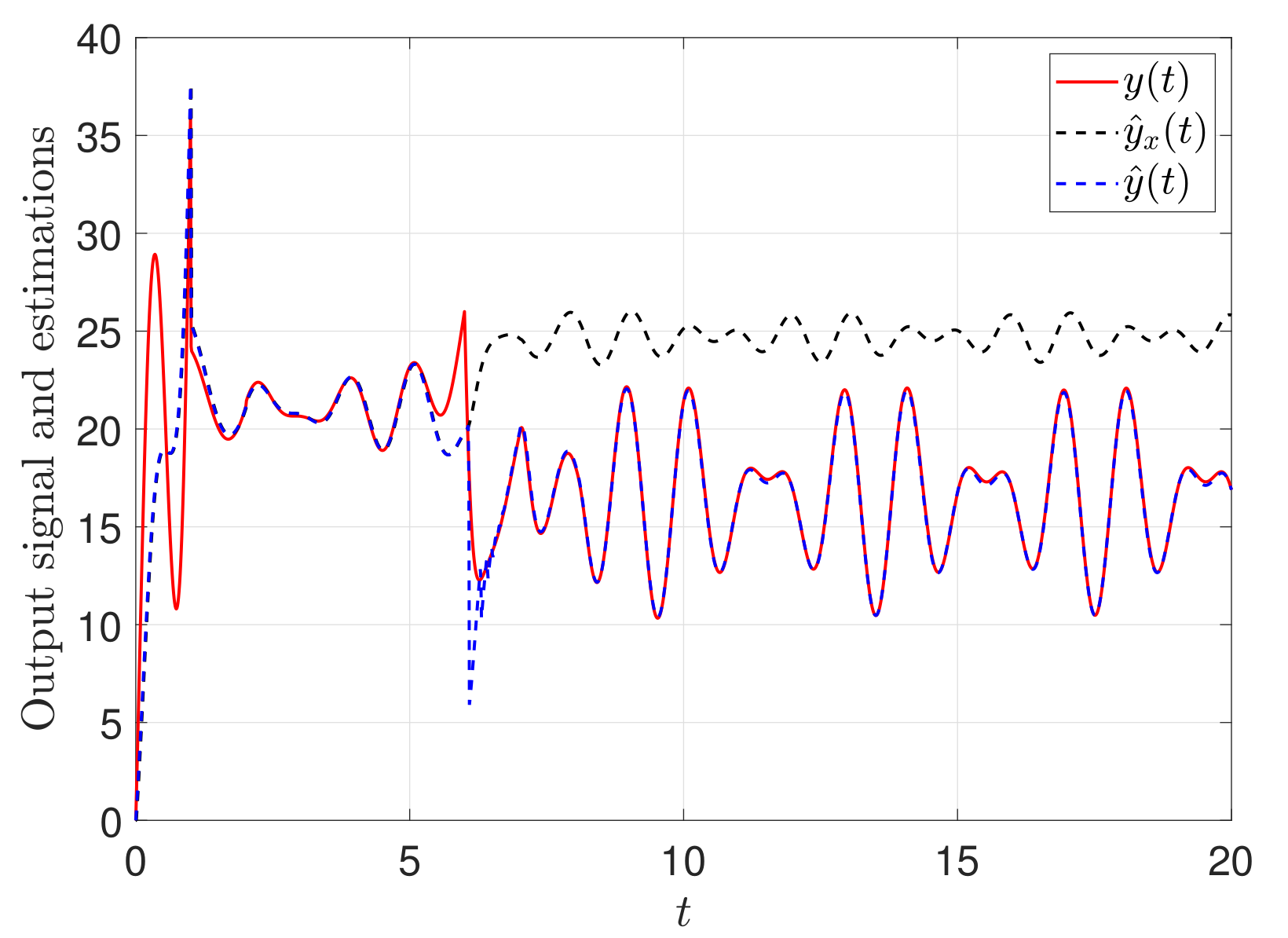
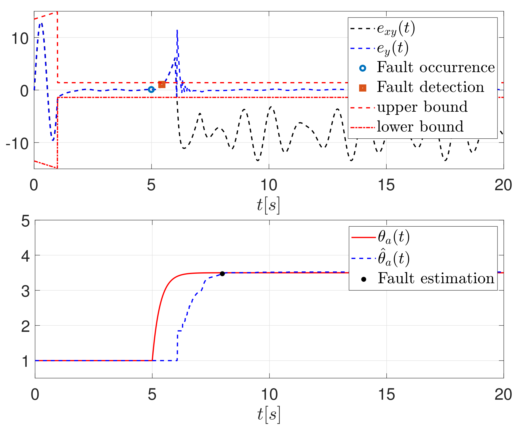
4.1.1. Actuator Fault Estimation

We simulate the system in the case of [p1]. The actuator fault occurs at $T_o=5s$ and becomes constant after $T=8s$. In Figure 2, the oscillation arises due to the perturbation $\varphi \left(t\right)={\varphi }_1$ as shown in Table 1. Applying the adaptation law (44) ensures that in Figure 2 the estimate $\widehat{y}\left(t\right)(0,t)=\widehat{v}$ (blue dotted line) converges to the measurement $y\left(t\right)$(solid line). As shown in Figure 3, the estimate ${\widehat{\theta }}_a\left(t\right)$ is exponentially convergent. We also use the common Lunberger observer (35)–(37), but the estimate ${\widehat{y}}_x\left(t\right)$ (black dotted line) deviates from the measurement. Particularly, the mean square error (MSE) is calculated for the output estimates to show performance.

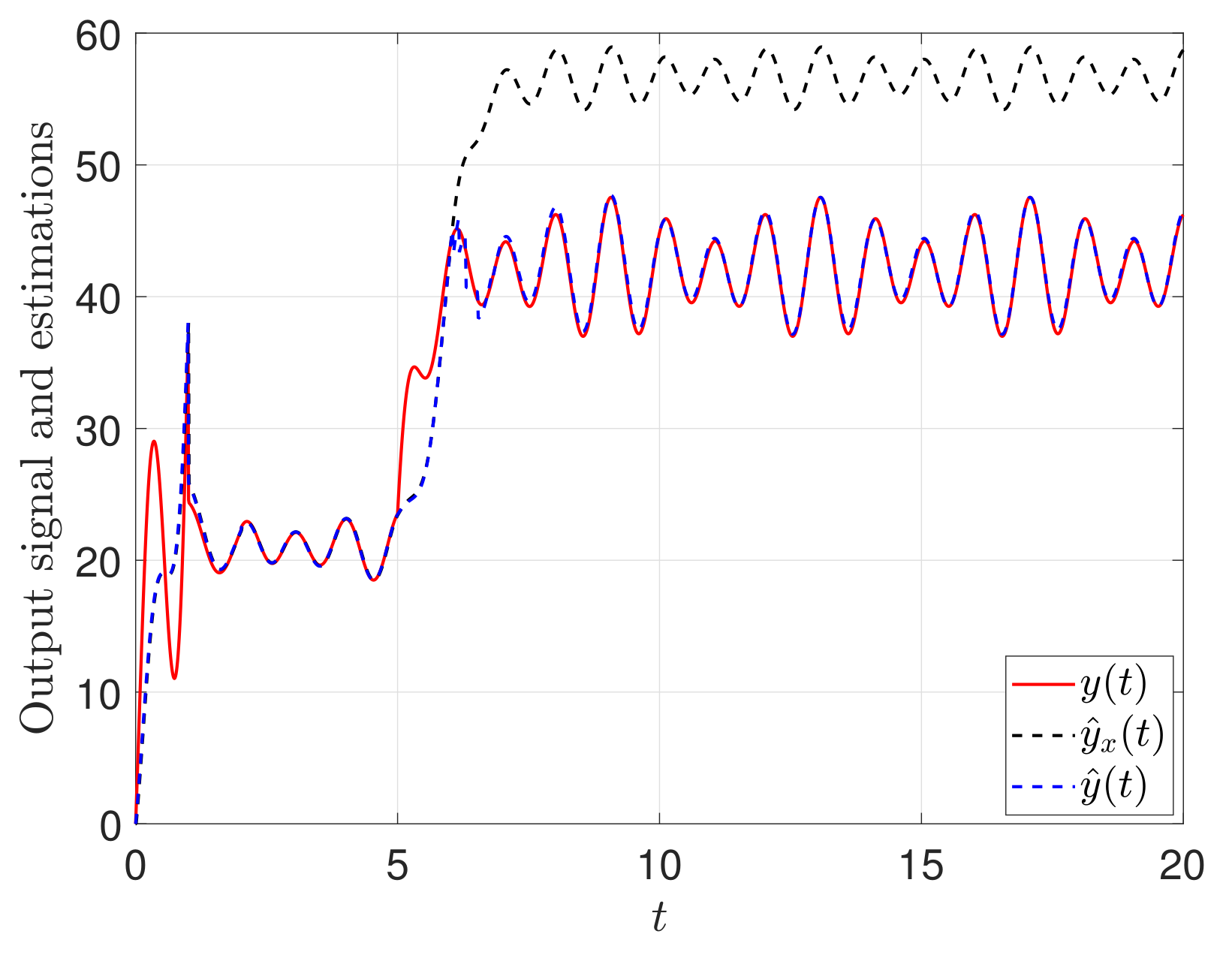
4.1.2. Sensor Fault Estimation

In this subsection, we investigate the performance of the proposed observer (40) and (41) and the adaptive law (46). We simulate the situation when the same system fails. Sensor fault occurs at $T_o=5s$, and is kept unchanging after $t=6s$. A new external perturbation $\varphi ={\varphi }_2$ shown in

Table 2. Fault occurrences, proposed observers, adaptive laws (AL) and design parameters.

Fault Occurrence	${\mathit{\theta }}_{\mathit{a}}$	${\mathit{\theta }}_{\mathit{s}}$	Observer	AL	$\mathit{\beta }$		$\mathit{\gamma }$
[p1]	★	-	(38)–(39)	(44)	91		0.03
[p2]	-	★	(40)–(41)	(46)	12		0.05
							${\gamma }_a$	${\gamma }_s$
[p3]	★	★	(42)–(43)	(75)–(76)	51		0.02	0.07

effects the system, where ‘★’ indicates the fault occurrences and ‘-’ shows no faults. A comparison between ${\widehat{y}}_x\left(t\right)$ and $\widehat{y}\left(t\right)={\widehat{\theta }}_s\left(t\right)\widehat{v}(0,t)$, see Figure 4 and Figure 5, where ${\widehat{y}}_x\left(t\right)$ is generated by the common Lunberger observer (35)–(37) and $\widehat{y}\left(t\right)$ is from the recommended observer (40) and (41). Apparently, the $\widehat{y}\left(t\right)$ (blue dashed line) exponentially converges to the measurement and the resulting residual $e_y\left(t\right)$ exponentially decays to a very small value in Figure 5. However, the common Lunberger observer (35)–(37) fails to give satisfactory results.

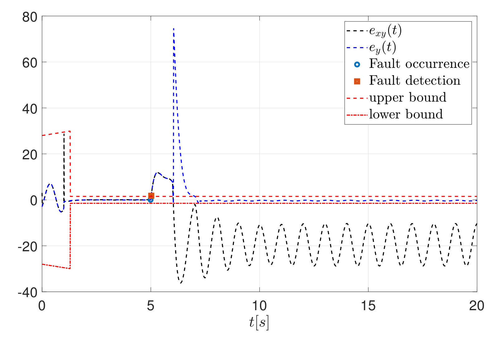
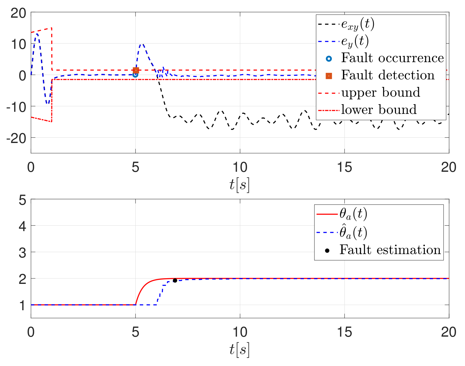
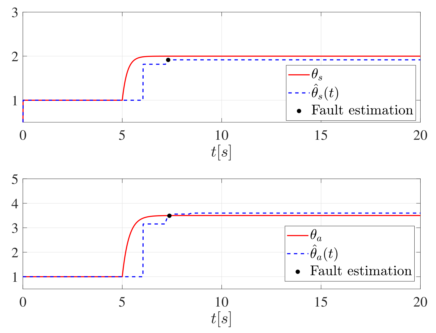
4.1.3. Simultaneous Fault Estimation

In this section, we carry out a simulation with the fault [P3]: both actuator and sensor faults occur at $T_o=5s$ and remain unchanged after $T=8s$. $\varphi \left(t\right)={\varphi }_3$ is the external disturbance defined in Table 1. We apply the adaptive observer (42) and (43) and coupling parameter adaptive law (75) and (76). Expected state estimates $\widehat{v}\left(\xi \right)$, ${\widehat{\theta }}_a$ and ${\widehat{\theta }}_s$ converge to $v\left(\xi \right)$, ${\theta }_a$ and ${\theta }_s$. The results in Figure 6 and Figure 7 directly show the performance of the proposed method.The observation error generated by the proposed observer (42) and (43) $\tilde{v}(0,t)=v(z,t)-\widehat{v}(z,t)$ and the residual $e_y\left(t\right)$ attenuates to a very small value around zero: see the dashed blue line in the Figure 6. However, the common observer (35)–(37) is unable to provide acceptable estimates as shown in the black dotted line in the Figure 6.

5. Conclusions

We propose a strategy to address the estimation problem of a class of linear hyperbolic PDE systems with single and simultaneous faults and unknown disturbance. The proposed observer implements state estimation and fault parameter estimation using the boundary measurement. The detailed observer design results are presented, and the unknown faults are estimated with parameter adaptation laws. Through numerical simulations, it is shown that the proposed parameter adaptation laws ensure arbitrarily small errors in the fault parameter estimation, despite the presence of unknown external disturbances. However, the common Lunberger observer fails to provide the exact state estimates when facing the faulty system. This method has the advantages of easy design and strong portability. Once the observer canonical form can be obtained, it is possible to extend the results of this work to more complex PDE systems. In this paper, we obtain that the error of fault parameters and state estimation is ultimately bounded.