Solution of Exterior Quasilinear Problems Using Elliptical Arc Artificial Boundary

Abstract

In this paper, the method of artificial boundary conditions for exterior quasilinear problems in concave angle domains is investigated. Based on the Kirchhoff transformation, the exact quasiliner elliptical arc artificial boundary condition is derived. Using the approximate elliptical arc artificial boundary condition, the finite element method is formulated in a bounded region. The error estimates are obtained. The effectiveness of our method is showed by some numerical experiments.

1. Introduction

In many fields of scientific and engineering computing, such as heat transfer, magnetostatics or compressible flow, it is necessary to deal with problems in unbounded domains. The method of artificial boundary conditions [1,2], which is also named coupled of finite element method and natural boundary element method [3,4,5] or DtN finite element method [6,7], is a normal method used to solve this kind of problem numerically.

The method can be summarized in the following four steps: (i) By introducing an artificial boundary ${\Gamma }_R$, truncate the original infinite domain $\Omega$ into two subdomains: a finite computational subdomain ${\Omega }_i$ and an unbounded residual subdomain ${\Omega }_e$. (ii) By dissecting the problem in ${\Omega }_e$, obtain a relation on ${\Gamma }_R$ involving the solution $u$ and its derivatives. (iii) Use the relation as an approximate boundary condition on ${\Gamma }_R$, to earn a well posed problem confined in ${\Omega }_i$. (iv) Use finite element method or other numerical methods to solve the problem in ${\Omega }_i$.

The relation derived in (ii) and used in (iii) is called an artificial boundary condition, natural integral equation or DtN map. Natural boundary reduction reduces the boundary value problem into a hypersingular integral equation on the artificial boundary. It has many advantages, such as the positive-definite symmetry of stiffness matrices, the stability of approximate solutions, and can be coupled with the finite element method naturally and directly. The method has been used to solve linear problems in last century. It has also been successfully extended to nonlinear problems in recent years.

Suppose $\Omega$ is an infinite domain with a concave angle $\alpha$, and $0<\alpha \le 2\pi$. The boundaries of $\Omega$ are disintegrated into three disjoint parts: ${\Gamma }_0$, ${\Gamma }_{\alpha }$ and $\Gamma$ (see Figure 1), i.e., $\partial \Omega ={\Gamma }_0\cup {\Gamma }_{\alpha }\cup \Gamma$, ${\Gamma }_0\cap {\Gamma }_{\alpha }=\varnothing$, ${\Gamma }_0\cap \Gamma =\varnothing$ and ${\Gamma }_{\alpha }\cap \Gamma =\varnothing$. The boundary $\Gamma$ is a simple smooth curve part, ${\Gamma }_0$ and ${\Gamma }_{\alpha }$ are two half lines.

We consider the following quasilinear problem

$$\{\begin{array}{c}-\nabla ·\left(a\left(x,u\right)\nabla u\right)=f, \mathrm{in}\Omega ,\\ \begin{array}{c}\frac{\partial u}{\partial n}=0, \mathrm{on} {\Gamma }_0\cup {\Gamma }_{\alpha },\\ u=0, \mathrm{on} \Gamma ,\end{array}\\ u\left(x\right) \mathrm{is} \mathrm{bounded}, \mathrm{as} \left|x\right|\to \infty ,\end{array}$$

(1)

where $a\left(x,u\right)$ and $f$ are given functions with some properties which will be decribed later.

Problem (1) has numerous physical applications, e.g., in the field of magnetostatics, where $u$ is the magnetic scalar potential and $a$ is the magnetic permeability; in the field of compressible flow, where $u$ is the velocity potential and $a$ is the density. There have been many numerical results about problems of this kind in bounded domains, for example, the existence and uniqueness of weak solution [8,9], the finite element method [10,11,12], the mixed finite element method [13,14,15], the discontinuous Galerkin finite element method [16,17,18], the weak Galerkin finite element method [19], and the adaptive finite element method [20,21].

The circular artificial boundary was used for exterior quasilinear problems in early years [22,23]. The elliptical artificial boundary was generalised later for elongated domains problems [24]. The circular arc boundary was often selected for problems in unbounded domains with concave angles [25], but for the problems in elongated concave angle domains, an elliptical arc boundary which leads to a smaller computational domain is much better than the circular arc case (see Figure 2).

In this paper, we propose a new method of elliptical arc artificial boundary conditions for the numerical solution of quasilinear problems in exterior elongated domains with concave angles.

Suppose that the given function $a\left(·,·\right)$ satisfies [8]

$$C_0\le a\left(x,u\right)\le C_1, \forall u\in ℝ, \mathrm{and} \mathrm{for} \mathrm{almost} \mathrm{all} x\in \Omega ,$$

(2)

and

$$\left|a\left(x,u\right)-a\left(x,v\right)\right|\le C_L\left|u-v\right|, \forall u,v\in ℝ, \mathrm{and} \mathrm{for} \mathrm{almost} \mathrm{all} x\in \Omega ,$$

(3)

where $C_0,C_1$ and $C_L$ are three positive constants. We also assume that $\frac{\partial a}{\partial \mathrm{s}}$, $\frac{{\partial }^{2}a}{\partial {\mathrm{s}}^2}$ are continuous. Additionally, we suppose that $f\in L^2(\Omega )$ has compact support, i.e., there exists a constant ${\mu }_0>0$, such that

$$\mathrm{supp}f\subset {\Omega }_{{\mu }_0}=\{x\in {ℝ}^2|\left|x\right|\le {\mu }_0\}.$$

(4)

Moreover, we assume that

$$a\left(x,u\right)\equiv a_0\left(u\right), \mathrm{when} \left|x\right|\ge {\mu }_0.$$

(5)

The rest of this paper is organized as follows. We derive the exact quasilinear elliptical arc artificial boundary condition in Section 2. In Section 3, we formulate the finite element approximation and give an new error estimate. In Section 4, we give some numerical experiments to show the efficiency and feasibility of our method. Some conclusions are given in Section 5.

In the following sections, we denote $C$ as a general positive constant independent of ${\mu }_1$, $N$ and $h$, where $N$ and $h$ will be defined in Section 2 and Section 3, respectively. The constant $C$ has different meaning in different place.

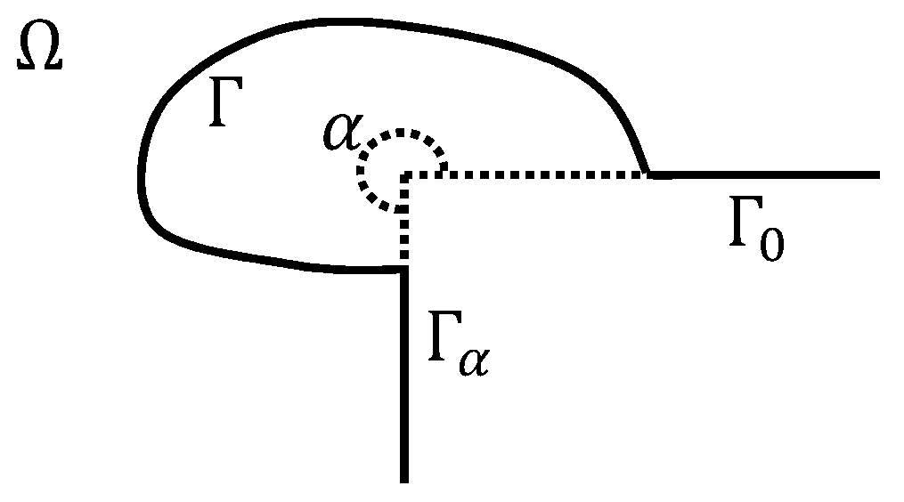
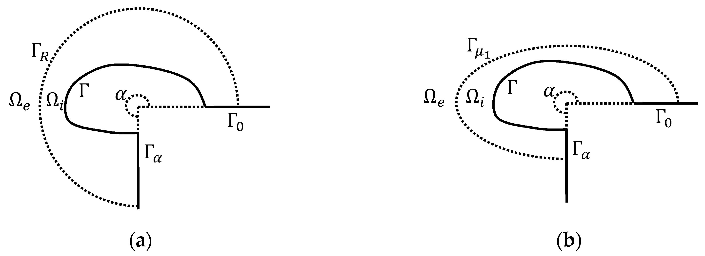
2. Exact Quasilinear Elliptical Arc Artificial Boundary Condition

We first introduce the elliptical arc artificial boundary ${\Gamma }_{{\mu }_1}=\{\left(x,y\right)|\frac{x^2}{a^2}+\frac{y^2}{b^2}=1,\left(x,y\right)\in \Omega ,a>b>0\}$ to enclose $\mathrm{supp}f$, which divides $\Omega$ into a bounded computational domain ${\Omega }_i$ and an unbounded domain ${\Omega }_e$ (see Figure 2b). Let $2f_0$ denote the distance between two foci of the previous ellipse, we introduce the elliptic co-ordinates $\left(\mu ,\phi \right)$ such that artificial boundary ${\Gamma }_{{\mu }_1}$ coincides with elliptical arc $\left\{\left(\mu ,\phi \right)\right|\mu ={\mu }_1, 0<\phi <\alpha \}$, where $f_0=\sqrt{a^2-b^2}$, ${\mu }_1=\ln \frac{a+b}{\sqrt{a^2-b^2}}$. Thus, the Cartesian co-ordinates $\left(x,y\right)$ are related to the elliptic co-ordinates $\left(\mu ,\phi \right)$, that is $x=f_0\cos \mathrm{h}\mu \cos \phi$, $y=f_0\sin \mathrm{h}\mu \sin \phi$.

Then, problem (1) can be rewritten in the following coupled form:

$$\{\begin{array}{c}-\nabla ·\left(a\left(x,u\right)\nabla u\right)=f, \mathrm{in}{\Omega }_i,\\ \frac{\partial u}{\partial n}=0, \mathrm{on} {\Gamma }_{0i}\cup {\Gamma }_{\alpha i},\\ u=0, \mathrm{on} \Gamma ,\end{array}$$

(6)

$$\{\begin{array}{c}-\nabla ·\left(a_0\left(u\right)\nabla u\right)=0, \mathrm{in}{\Omega }_e,\\ \frac{\partial u}{\partial n}=0, \mathrm{on} {\Gamma }_{0e}\cup {\Gamma }_{\alpha e},\\ u\left(x\right) \mathrm{is} \mathrm{bounded}, \mathrm{as} \left|x\right|\to \infty ,\end{array}$$

(7)

$$u\left(x\right) \mathrm{and} a_0\left(u\right)\frac{\partial u}{\partial n} \mathrm{are} \mathrm{continuous} \mathrm{on} \mathrm{the} \mathrm{artificial} \mathrm{boundary} {\Gamma }_{{\mu }_1},$$

(8)

where ${\Gamma }_{0i}={\Gamma }_0\cap {\Omega }_i$, ${\Gamma }_{\alpha i}={\Gamma }_{\alpha }\cap {\Omega }_i$, ${\Gamma }_{0e}={\Gamma }_0\cap {\Omega }_e$, and ${\Gamma }_{\alpha e}={\Gamma }_{\alpha }\cap {\Omega }_e$.

We introduce the so-called Kirchhoff transformation [26]:

$$w\left(x\right)={\int }_0^{u\left(x\right)}{a}_0\left(\xi \right)d\xi , \mathrm{for} x\in {\Omega }_e.$$

(9)

The transformation is invertible because $a_0\left(u\right)$ is a positive function. Notice that

$$\nabla w=a_0\left(u\right)\nabla u,$$

(10)

we can transform the quasilinear problem (7) into the following linear problem

$$\{\begin{array}{c}-\Delta w=0, \mathrm{in}{\Omega }_e,\\ \frac{\partial w}{\partial n}=0, \mathrm{on} {\Gamma }_{0e}\cup {\Gamma }_{\alpha e},\\ w\left(x\right) \mathrm{is} \mathrm{bounded}, \mathrm{as} \left|x\right|\to \infty .\end{array}$$

(11)

Suppose $w\left(x\right)$ is the solution of problem (11). By Fourier series expansion, we have

$$w\left(\mu ,\phi \right)=\frac{b_0}{2}+{\sum }_{n=1}^{+\infty }{b}_n{e}^{\left({\mu }_1-\mu \right)\frac{n\pi }{\alpha }}\cos \frac{n\pi \phi }{\alpha },$$

(12)

where

$$b_n=\frac{2}{\alpha }{\int }_0^{\alpha }w\left({\mu }_1,\varphi \right)\cos \frac{n\pi \varphi }{\alpha }d\varphi , n=0,1,2,\cdots .$$

(13)

It is easy to obtain

$$\frac{\partial w}{\partial \mu }\left(\mu ,\phi \right){|}_{\mu ={\mu }_1}=-\frac{2\pi }{{\alpha }^2}{\sum }_{n=1}^{+\infty }n{\int }_0^{\alpha }w\left({\mu }_1,\varphi \right)\cos \frac{n\pi \varphi }{\alpha }\cos \frac{n\pi \phi }{\alpha }d\varphi .$$

(14)

Since

$$\frac{\partial w}{\partial n}=-\frac{1}{\sqrt{J_0}}\frac{\partial w}{\partial \mu },$$

(15)

where $J_0=f_0^2\left({\cos \mathrm{h}}^2{\mu }_1-{\cos }^2\phi \right)$, and

$$\frac{\partial w}{\partial n}=a_0\left(u\right)\frac{\partial u}{\partial n},$$

(16)

we obtain the exact artificial boundary condition of $u$ on ${\Gamma }_{{\mu }_1}$:

$$a_0\left(u\right)\frac{\partial u}{\partial n}=\frac{2\pi }{{\alpha }^2\sqrt{J_0}}{\sum }_{n=1}^{+\infty }n{\int }_0^{\alpha }({\int }_0^{u\left({\mu }_1,\varphi \right)}{a}_0\left(y\right)dy)\cos \frac{n\pi \varphi }{\alpha }\cos \frac{n\pi \phi }{\alpha }d\varphi \triangleq \mathcal{K}u\left({\mu }_1,\phi \right).$$

(17)

The difference between this artificial boundary condition and that in circular arc case is only a factor $\frac{1}{\sqrt{J_0}}$ [25], so it does not increase the computational complexity of the stiff matrix from artificial boundary. In the meantime, an elliptical arc artificial boundary is advantageous in that it may be used to enclose some narrow region with concave angle efficiently, so it is much better than the circular arc one.

By the exact quasilinear artificial boundary condition (17), we have

$$\{\begin{array}{c}-\nabla ·\left(a\left(x,u\right)\nabla u\right)=f, \mathrm{in}{\Omega }_i,\\ \begin{array}{c}\frac{\partial u}{\partial n}=0, \mathrm{on} {\Gamma }_{0i}\cup {\Gamma }_{\alpha i},\\ u=0, \mathrm{on} \Gamma ,\end{array}\\ a_0\left(u\right)\frac{\partial u}{\partial n}=\mathcal{K}u\left({\mu }_1,\phi \right), \mathrm{on} {\Gamma }_{{\mu }_1}.\end{array}$$

(18)

Let $V=\{v\in H^1\left({\Omega }_i\right)|v{|}_{\Gamma }=0\}$, then problem (18) is equivalent to the variational problem as follows:

$$\{\begin{array}{c}\mathrm{Find} u\in V, \mathrm{such} \mathrm{that}\\ A\left(u;u,v\right)+B\left(u;u,v\right)=F\left(v\right), \forall v\in V,\end{array}$$

(19)

where

$$A\left(w;u,v\right)={\int }_{{\Omega }_i}^{}a\left(x,w\right)\nabla u·\nabla vdx,$$

(20)

$$B\left(w;u,v\right)={\sum }_{n=1}^{+\infty }\frac{2}{n\pi }{\int }_0^{\alpha }{\int }_0^{\alpha }{a}_0\left(w\left({\mu }_1,\varphi \right)\right)\frac{\partial u}{\partial \varphi }\left({\mu }_1,\varphi \right)\frac{\partial v}{\partial \phi }\left({\mu }_1,\phi \right)\sin \frac{n\pi \varphi }{\alpha }\sin \frac{n\pi \phi }{\alpha }d\varphi d\phi ,$$

(21)

$$F\left(v\right)={\int }_{{\Omega }_i}^{}f\left(x\right)v\left(x\right)dx.$$

(22)

In practice, we must truncate the infinite series in (17) by finite terms, let

$${\mathcal{K}}^{N}u=\frac{2\pi }{{\alpha }^2\sqrt{J_0}}{\sum }_{n=1}^{N}n{\int }_0^{\alpha }({\int }_0^{u\left({\mu }_1,\varphi \right)}{a}_0\left(y\right)dy)\cos \frac{n\pi \varphi }{\alpha }\cos \frac{n\pi \phi }{\alpha }d\varphi .$$

(23)

Consider the following approximation problem:

$$\{\begin{array}{c}-\nabla ·\left(a\left(x,u^N\right)\nabla u^N\right)=f, \mathrm{in}{\Omega }_i,\\ \begin{array}{c}\frac{\partial u^N}{\partial n}=0, \mathrm{on} {\Gamma }_{0i}\cup {\Gamma }_{\alpha i},\\ u^N=0, \mathrm{on} \Gamma ,\end{array}\\ a_0\left(u^N\right)\frac{\partial u^N}{\partial n}={\mathcal{K}}^N{u}^N, \mathrm{on} {\Gamma }_{{\mu }_1}.\end{array}$$

(24)

It is equivalent to the variational problem as follows:

$$\{\begin{array}{c}\mathrm{Find} u^N\in V, \mathrm{such} \mathrm{that}\\ A\left(u^N;u^N,v\right)+B_N\left(u^N;u^N,v\right)=F\left(v\right), \forall v\in V,\end{array}$$

(25)

where

$$B_N\left(w;u,v\right)={\sum }_{n=1}^N\frac{2}{n\pi }{\int }_0^{\alpha }{\int }_0^{\alpha }{a}_0\left(w\left({\mu }_1,\varphi \right)\right)\frac{\partial u}{\partial \varphi }\left({\mu }_1,\varphi \right)\frac{\partial v}{\partial \phi }\left({\mu }_1,\phi \right)\sin \frac{n\pi \varphi }{\alpha }\sin \frac{n\pi \phi }{\alpha }d\varphi d\phi .$$

(26)

For $s\in ℝ$, we introduce the equivalent definition of Sobolev spaces $H^s\left({\Gamma }_{{\mu }_1}\right)$ as follows [27]:

$$\forall H^s\left({\Gamma }_{{\mu }_1}\right)\iff v\left({\mu }_1,\phi \right)=\frac{b_0}{2}+{\sum }_{n=1}^{+\infty }{b}_n\cos \frac{n\pi \phi }{\alpha } \mathrm{and} \frac{b_0^2}{2}+{\sum }_{n=1}^{+\infty }{\left(1+n^2\right)}^s{b}_n^2<\infty .$$

The norm of $H^s\left({\Gamma }_{{\mu }_1}\right)$ can be defined as follows:

$$\parallel v{\left({\mu }_1,\phi \right)\parallel }_{s,{\Gamma }_{{\mu }_1}}={\left[\frac{b_0^2}{2}+{\sum }_{n=1}^{+\infty }{\left(1+n^2\right)}^s{b}_n^2\right]}^{\frac{1}{2}}.$$

Then, we have the following results.

Lemma 1. 

$B\left(u;u,v\right)$and$B_N\left(u;u,v\right)$are both a symmetric, semi-definite and continuous bilinear form on$V\times V$.

Proof. 

For $u,v\in V$, we assume that

$$u\left({\mu }_1,\varphi \right)=\frac{b_0}{2}+{\sum }_{n=1}^{+\infty }{b}_n\cos \frac{n\pi \varphi }{\alpha },$$

$$v\left({\mu }_1,\phi \right)=\frac{d_0}{2}+{\sum }_{n=1}^{+\infty }{d}_n\cos \frac{n\pi \phi }{\alpha },$$

taking the derivative with respect to $\varphi$ and $\phi$, we obtain

$$\frac{\partial u}{\partial \varphi }\left({\mu }_1,\varphi \right)={\sum }_{n=1}^{+\infty }\frac{n\pi }{\alpha }{b}_n\sin \frac{n\pi \varphi }{\alpha },$$

$$\frac{\partial v}{\partial \phi }\left({\mu }_1,\phi \right)={\sum }_{n=1}^{+\infty }\frac{n\pi }{\alpha }{d}_n\sin \frac{n\pi \phi }{\alpha },$$

then we have

$$\begin{array}{c}\hfill \left|B\left(u;u,v\right)\right|\le C{\left({\sum }_{n=1}^{+\infty }n{b}_n^2\right)}^{\frac{1}{2}}{\left({\sum }_{n=1}^{+\infty }n{d}_n^2\right)}^{\frac{1}{2}}\hfill \\ \hspace{1em}\hspace{1em}\hspace{1em}\le C{\parallel u\parallel }_{\frac{1}{2},{\Gamma }_{{\mu }_1}}{\parallel v\parallel }_{\frac{1}{2},{\Gamma }_{{\mu }_1}}\le C{\parallel u\parallel }_{1,{\Omega }_i}{\parallel v\parallel }_{1,{\Omega }_i}.\end{array}$$

In the same way, we obtain

$$\left|B_N\left(u;u,v\right)\right|\le C{\left({\sum }_{n=1}^{N}n{b}_n^2\right)}^{\frac{1}{2}}{\left({\sum }_{n=1}^{N}n{d}_n^2\right)}^{\frac{1}{2}}\le C{\parallel u\parallel }_{1,{\Omega }_i}{\parallel v\parallel }_{1,{\Omega }_i}.$$

Next, we show that $B\left(u;u,v\right)$ and $B_N\left(u;u,v\right)$ are semi-definite. For any given $v\in V$, we consider the following auxiliary problem:

$$\{\begin{array}{c}-\nabla ·\left(a\left(x,u\right)\nabla u\right)=0, \mathrm{in}{\Omega }_e,\\ \begin{array}{c}\frac{\partial u}{\partial n}=0, \mathrm{on} {\Gamma }_{0e}\cup {\Gamma }_{\alpha e},\\ u=v, \mathrm{on} {\Gamma }_{{\mu }_1},\end{array}\\ u\left(x\right) \mathrm{is} \mathrm{bounded}, \mathrm{as} \left|x\right|\to \infty , \end{array}$$

(27)

the solution $u$ of the above problem satisfies

$$a_0\left(u\right)\frac{\partial u}{\partial n}=\mathcal{K}u\left({\mu }_1,\phi \right).$$

If we multiply (27) by $u$ and integrate over ${\Omega }_e$, then we can obtain

$$B\left(u;u,u\right)={\int }_{{\Omega }_e}^{}{a}_0\left(u\right){\left|\nabla u\right|}^{2}dx\ge 0.$$

In the same way, we obtain

$$B_N\left(u;u,u\right)\ge 0.$$

This completes the proof. □

3. Finite Element Approximation

Suppose ${\mathcal{J}}_h$ is a regular and quasi-uniform triangulation on ${\Omega }_i$, s.t.

$${\Omega }_i={\cup }_{K\in {\mathcal{J}}_h}K,$$

(28)

where $K$ is a (curved) triangle, $h$ denote the maximal side of the triangles. Let

$$V_h=\{v_h\in V,v_h| K \mathrm{is} \mathrm{a} \mathrm{linear} \mathrm{polynomial}, \forall K\in {\mathcal{J}}_h\}.$$

(29)

Then, the approximation problem of (25) is

$$\{\begin{array}{c}\mathrm{Find} u_h^N\in V_h, \mathrm{such} \mathrm{that}\\ A\left(u_h^N;u_h^N,v_h\right)+B_N\left(u_h^N;u_h^N,v_h\right)=F\left(v_h\right), \forall v_h\in V_h.\end{array}$$

(30)

Lemma 2. 

The variational problems (19), (25) and (30) are uniquely solvable.

Proof. 

From (2), it is easy to shown that the bilinear form $A\left(u;u,v\right)$ is $V$-elliptic and bounded in $V$, i.e., there exist constants $C_0,C_1>0$, such that

$$\left|A\left(u;v,v\right)\right|\ge C_0{\parallel v\parallel }_{1,{\Omega }_i}^2,$$

$$\left|A\left(u;u,v\right)\right|\le C_1{\parallel u\parallel }_{1,{\Omega }_i}{\parallel v\parallel }_{1,{\Omega }_i}.$$

Combining with Lemma 1, we can deduce that $A\left(u;u,v\right)+B\left(u;u,v\right)$ is also $V$-elliptic and bounded in $V$. By (3), $a\left(x,u\right)$ is uniformly Lipschitz continuous with respect to $u$. Since these conditions hold, it is known [8] that variational problem (19) has a unique solution $u\in V$ for all $f\in L^2(\Omega )$. In the same way, we obtain that the variational problems (25) and (30) are uniquely solvable. □

We let $u,u^N\in H^2\left({\Omega }_i\right)$ and $u_h\in V_h$ be the solution of problems (19), (25) and (30), respectively. We also assume that

$$V_h\subset V\cap W^{1,2+\epsilon }\left({\Omega }_i\right) \mathrm{for} \mathrm{some} \epsilon \in \left(0,1\right).$$

(31)

Moreover, we require that ${\left\{V_h\right\}}_{h\to 0}$ is a family of finite dimensional subspaces of $V \cap C\left({\Omega }_i\right)$, s.t.

$$v\in V \cap C\left({\Omega }_i\right), \mathrm{there} \mathrm{exists} \left\{v_h\right\} :v_h\in V_h, \parallel v-v_h\parallel \to 0, \mathrm{as} h\to 0,$$

(32)

$$\parallel v_h\parallel {}_{1,2+\epsilon ,{\Omega }_i}\le C\left(v\right) \mathrm{for} \mathrm{any} h,$$

(33)

where $C\left(v\right)>0$ is independent of $h$.

It is obvious that the continuous piecewise polynomial spaces (29) satisfy (31). Furthermore, if we suppose $v_h={\Pi }_{h}v$, and ${\Pi }_h:v\to v_h$ is the interpolation operator, we have

$$\parallel v_h\parallel {}_{1,2+\epsilon ,{\Omega }_i}\le \parallel {\Pi }_{h}v-{v\parallel }_{1,2+\epsilon ,{\Omega }_i}+{\parallel v\parallel }_{1,2+\epsilon ,{\Omega }_i}\le C\left(v\right).$$

Following the convergence theory in [5,8], we have the following result:

$$\underset{h\to 0}{\lim }\parallel u_h^N-u^N\parallel {}_{1,{\Omega }_i}=0 \mathrm{and} u^N\subset V \cap W^{1,2+\epsilon }\left({\Omega }_i\right), \forall N\ge 0.$$

(34)

Moreover, we can obtain the following lemma.

Lemma 3. 

Suppose$u$be the solution of (19) and$u^N$be the solution of (25). Then, we have

$$\underset{N\to +\infty }{\lim }\parallel u-u^N{\parallel }_{1,{\Omega }_i}=0.$$

(35)

Proof. 

From (2) and Lemma 2, we have

$$\begin{array}{cc}\hfill \parallel u^N\parallel {}_{1,{\Omega }_i}^2\le \hfill & C\left(A\left(u^N;u^N,u^N\right)+B\left(u^N;u^N,u^N\right)\right)\hfill \\ & =C\left(F\left(u^N\right)+B\left(u^N;u^N,u^N\right)-B_N\left(u^N;u^N,u^N\right)\right)\hfill \\ & \le C\left({\parallel f\parallel }_{0,{\Omega }_i}·{\parallel u}^N\parallel {}_{1,{\Omega }_i}+\left|B\left(u^N;u^N,u^N\right)-B_N\left(u^N;u^N,u^N\right)\right|\right)\hfill \end{array}$$

For $u^N\in V$, we assume that

$$w^N\left(\mu ,\varphi \right)={\int }_0^{u^N\left(\mu ,\varphi \right)}{a}_0\left(\xi \right)d\xi =\frac{b_0}{2}+{\sum }_{n=1}^{+\infty }{b}_n{e}^{\left({\mu }_0-\mu \right)\frac{n\pi }{\alpha }}\cos \frac{n\pi \varphi }{\alpha }, \forall \mu >{\mu }_0,$$

$$u^N\left({\mu }_1,\phi \right)=\frac{d_0}{2}+{\sum }_{n=1}^{+\infty }{d}_n\cos \frac{n\pi \phi }{\alpha },$$

then we have

$$\begin{array}{cc}& \left|B\left(u^N;u^N,u^N\right)-B_N\left(u^N;u^N,u^N\right)\right|\hfill \\ \hfill =\hfill & \left|{\sum }_{n=N+1}^{+\infty }\frac{2}{n\pi }{\int }_0^{\alpha }{\int }_0^{\alpha }\frac{\partial w^N}{\partial \varphi }\left({\mu }_1,\varphi \right)\frac{\partial u^N}{\partial \phi }\left({\mu }_1,\phi \right)\sin \frac{n\pi \varphi }{\alpha }\sin \frac{n\pi \phi }{\alpha }d\varphi d\phi \right|\hfill \\ \hfill =\hfill & \parallel {\sum }_{n=N+1}^{+\infty }\frac{n\pi }{2}{e}^{\left({\mu }_0-{\mu }_1\right)\frac{n\pi }{\alpha }}{b}_n{d}_n\parallel \hfill \\ \hfill \le \hfill & C{e}^{\left({\mu }_0-{\mu }_1\right)\frac{\left(N+1\right)\pi }{\alpha }}{\left({\sum }_{n=N+1}^{+\infty }n{b}_n^2\right)}^{\frac{1}{2}}{\left({\sum }_{n=N+1}^{+\infty }n{d}_n^2\right)}^{\frac{1}{2}}\hfill \\ \hfill \le \hfill & C{e}^{\left({\mu }_0-{\mu }_1\right)\frac{\left(N+1\right)\pi }{\alpha }}\parallel w^N\parallel {}_{\frac{1}{2},{\Gamma }_{{\mu }_0}}\parallel u^N\parallel {}_{\frac{1}{2},{\Gamma }_{{\mu }_1}}\hfill \\ \hfill \le \hfill & C{e}^{\left({\mu }_0-{\mu }_1\right)\frac{\left(N+1\right)\pi }{\alpha }}\parallel u^N\parallel {}_{1,{\Omega }_i}^2.\hfill \end{array}$$

From ${\mu }_1>{\mu }_0$, we deduce that $\left\{u^N\right\}$ is bounded in $V$. Therefore, we obtain a subsequence $\left\{u^{N_n}\right\}$, s.t. $u^{N_n}\rightharpoonup \overline{u}\in V$. Then, similar with Lemma 3.4 of [22], we have (35). □

Finally, we obtain the convergence result as follows.

Theorem 1. 

Suppose$u\in H^2\left({\Omega }_i\right)$, andletassumptions (31)–(33) be satisfied. Then, we have

$$\underset{h\to 0,N\to +\infty }{\lim }\parallel u-u_h^N\parallel {}_{1,{\Omega }_i}=0.$$

(36)

Next, we give the error estimates. We assume that the solution $u$ of problem (1) satisfies

$$u{|}_{{\Omega }_i}\in V \cap W^{k,2+\epsilon }\left({\Omega }_i\right), \epsilon >0, k\ge 2.$$

For simplicity, we define the following notation

$$D\left(u;u,v\right)\triangleq A\left(u;u,v\right)+B\left(u;u,v\right),$$

$$D_N\left(u^N;u^N,v\right)\triangleq A\left(u^N;u^N,v\right)+B_N\left(u^N;u^N,v\right),$$

$$D_N\left(u_h^N;u_h^N,v_h\right)\triangleq A\left(u_h^N;u_h^N,v_h\right)+B_N\left(u_h^N;u_h^N,v_h\right).$$

Then, problems (19), (25) and (30) can be reduced to the simple forms, respectively. Let us introduce the bilinear form $D^{\prime }\left(u;·,·\right)$ and $D_N^{\prime }\left(u^N;·,·\right)$ defined by

$$\begin{array}{c}\hfill D^{\prime }\left(u;v,z\right)={\int }_{{\Omega }_i}^{}\frac{\partial a}{\partial s}\left(x,u\right)v\nabla u·\nabla zdx+{\int }_{{\Omega }_i}^{}a\left(x,u\right)\nabla v·\nabla zdx\hfill \\ \hfill +{{\displaystyle \int }}_0^{\alpha }{{\displaystyle \int }}_0^{\alpha }\frac{\partial a_0}{\partial s}\left(u\right)v\frac{\partial u}{\partial \varphi }\left({\mu }_1,\varphi \right)\frac{\partial z}{\partial \phi }\left({\mu }_1,\phi \right){\displaystyle {\displaystyle \sum }_{n=1}^{+\infty }}\frac{2}{n\pi }\sin \frac{n\pi \varphi }{\alpha }\sin \frac{n\pi \phi }{\alpha }d\varphi d\phi \hfill \\ \hfill +{\int }_0^{\alpha }{\int }_0^{\alpha }{a}_0\left(u\right)\frac{\partial v}{\partial \varphi }\left({\mu }_1,\varphi \right)\frac{\partial z}{\partial \phi }\left({\mu }_1,\phi \right){\sum }_{n=1}^{+\infty }\frac{2}{n\pi }\sin \frac{n\pi \varphi }{\alpha }\sin \frac{n\pi \phi }{\alpha }d\varphi d\phi ,\hfill \end{array}$$

$$\begin{array}{c}\hfill D_N^{\prime }\left(u^N;v,z\right)={\int }_{{\Omega }_i}^{}\frac{\partial a}{\partial s}\left(x,u^N\right)v\nabla u^N·\nabla zdx+{\int }_{{\Omega }_i}^{}a\left(x,u^N\right)\nabla v·\nabla zdx\hfill \\ \hfill +{{\displaystyle \int }}_0^{\alpha }{{\displaystyle \int }}_0^{\alpha }\frac{\partial a_0}{\partial s}\left(u^N\right)v\frac{\partial u^N}{\partial \varphi }\left({\mu }_1,\varphi \right)\frac{\partial z}{\partial \phi }\left({\mu }_1,\phi \right){\displaystyle {\displaystyle \sum }_{n=1}^N}\frac{2}{n\pi }\sin \frac{n\pi \varphi }{\alpha }\sin \frac{n\pi \phi }{\alpha }d\varphi d\phi \hfill \\ \hfill +{\int }_0^{\alpha }{\int }_0^{\alpha }{a}_0\left(u^N\right)\frac{\partial v}{\partial \varphi }\left({\mu }_1,\varphi \right)\frac{\partial z}{\partial \phi }\left({\mu }_1,\phi \right){\sum }_{n=1}^N\frac{2}{n\pi }\sin \frac{n\pi \varphi }{\alpha }\sin \frac{n\pi \phi }{\alpha }d\varphi d\phi .\hfill \end{array}$$

Let $V^{\prime }$ denote the dual of $V$. Notice that $D^{\prime }\left(u;·,·\right)$ is bounded on $V\times V$ since (2) and $\frac{\partial a}{\partial s}\left(·,u(·)\right)$ are continuous. Then, we have an operator $T: V\to V^{\prime }$, s.t.

$$\left(Tv,z\right)=D^{\prime }\left(u;v,z\right), \forall v,z\in V.$$

(37)

Similar with Lemma 2.2 of [23], we have the following lemma.

Lemma 4. 

The bilinear form$\left(Tv,v\right)$defined by$D^{\prime }\left(u;v,v\right)$satisfies the following inequality

$$\left(Tv,v\right)+K\left({\parallel v\parallel }_{0,{\Omega }_i}^2+{\parallel v\parallel }_{\frac{1}{2},{\Gamma }_{{\mu }_1}}^2\right)\ge C{\parallel v\parallel }_{1,{\Omega }_i}^2, \forall v\in V,$$

(38)

where$K \ge 0$is a sufficient large constant.

We assume that

$$D^{\prime }\left(u;v,z\right)=0, \forall z\in V\Rightarrow v=0.$$

(39)

Let $I:V\to V^{\prime }$ denote the canonical injection. We obtain that operator $J:V\to V^{\prime }$ defined by $J\left(v\right)=\left(I\left(v\right),0\right)$ is also compact since $V$ is compactly embedded in $L^2\left({\Omega }_i\right)$. Thus the Fredholm alternative applies for $T$. We have that $T:V\to V^{\prime }$ is an isomorphism.

According to Theorem 10.1.2 of [28], under the conditions (19), (38) and (39), there exists an $h_0\in \left(0,1\right]$, such that the following inf-sup condition is satisfied.

$$\underset{z\in V_h}{\sup }\frac{D^{\prime }\left(u;v,z\right)}{{\parallel z\parallel }_{1,{\Omega }_i}}\ge {\alpha }_1{\parallel v\parallel }_{1,{\Omega }_i}, \forall v\in V_h,$$

(40)

for some constant ${\alpha }_1>0$ independent of $h(h<h_0)$.

We define the Galerkin projection with respect to $D^{\prime }\left(u;·,·\right)$, $P_h:V\to V_h$

$$D^{\prime }\left(u;P_{h}v,z\right)=D^{\prime }\left(u;v,z\right), \forall z\in V_h.$$

Then, we obtain

$$\parallel v-P_{h}v\parallel {}_{1,p,{\Omega }_i}\le C\underset{v_h\in V_h}{\inf }\parallel v-v_h\parallel {}_{1,p,{\Omega }_i}\le C{h}^{\sigma },$$

(41)

where $2\le p\le \infty , 0<\sigma <1.$

Lemma 5. 

$u_h^N\in V_h$is a solution of (30) if, and only if, this equation,

$$D_N^{\prime }\left(u^N;u^N-u_h^N,v\right)=R\left(u^N;u_h^N,v\right), \forall v\in V_h,$$

holds, where

$$\begin{array}{cc}& R\left(u^N;u_h^N,v\right)\hfill \\ \triangleq & {\int }_{{\Omega }_i}^{}({\int }_0^1\left(\frac{{\partial }^{2}a}{\partial s^2}\left(x,w_h^N\right)\nabla w_h^N·\nabla v\right)\left(1-t\right)dt){\left(d_h^N\right)}^{2}dx\hfill \\ +2& {\int }_{{\Omega }_i}^{}\left({\int }_0^1\left(\frac{\partial a}{\partial s}\left(x,w_h^N\right)\nabla d_h^N·\nabla v\right)\left(1-t\right)dt\right)d_h^{N}dx\hfill \\ +& {\int }_0^{\alpha }{\int }_0^{\alpha }\left({\int }_0^1\left(\frac{{\partial }^2{a}_0}{\partial s^2}\left(w_h^N\right)\frac{\partial w_h^N}{\partial \varphi }\frac{\partial v}{\partial \phi }{\sum }_{n=1}^N\frac{2}{n\pi }\sin \frac{n\pi \varphi }{\alpha }\sin \frac{n\pi \phi }{\alpha }\right)\left(1-t\right)dt\right){\left(d_h^N\right)}^{2}d\varphi d\phi \hfill \\ +2& {\int }_0^{\alpha }{\int }_0^{\alpha }\left({\int }_0^1\left(\frac{\partial a_0}{\partial s}\left(w_h^N\right)\frac{\partial d_h^N}{\partial \varphi }\frac{\partial v}{\partial \phi }{\sum }_{n=1}^N\frac{2}{n\pi }\sin \frac{n\pi \varphi }{\alpha }\sin \frac{n\pi \phi }{\alpha }\right)\left(1-t\right)dt\right)d_h^{N}d\varphi d\phi .\hfill \end{array}$$

with $w_h^N=u^N+t\left(u_h^N-u^N\right), d_h^N=u_h^N-u^N$.

Proof. 

Let $\eta \left(t\right)\triangleq D_N\left(w_h^N;w_h^N,v\right)$. Then, by (25), (30), and

$$\eta \left(1\right)=\eta \left(0\right)+{\eta }^{\prime }\left(0\right)+{\int }_0^1{\eta }^{″}\left(t\right)\left(1-t\right)dt,$$

we can get the desired result. □

Let

$$M_h\triangleq \left\{v\in V_{h|}{\parallel v\parallel }_{1,\infty ,{\Omega }_i}\le 1+\parallel u^N\parallel {}_{1,\infty ,{\Omega }_i}\right\},$$

(42)

Then, following [23,29], we have the Lemma as follows.

Lemma 6. 

There exists a constant$C>0$independent of$h$, such that

$$\left|R\left(u^N;v,z\right)\right|\le C(\parallel u^N-v{\parallel }_{1,{\Omega }_i}^2+\parallel u^N-v{\parallel }_{1,{\Omega }_i}){\parallel z\parallel }_{1,{\Omega }_i}, \forall v\in M_h, \forall z\in V_h.$$

We define a nonlinear mapping $\psi : V_h\to V_h$ as follows. $\psi \left(v\right)$ is the unique solution of

$$D^{\prime }\left(u;\psi \left(v\right),z\right)=D^{\prime }\left(u;u,z\right)-R\left(u;v,z\right), \forall z\in V_h,$$

(43)

for any given $v\in V_h$. Let

$$E_h\triangleq \left\{v\in V_{h|}\parallel v-P_h{v\parallel }_{1,\infty ,{\Omega }_i}\le C{h}^{\sigma }\right\},$$

(44)

then we have

Lemma 7. 

The nonlinear mapping$\psi$is continuousfrom$E_h$to$E_h$.

Proof. 

By (43), we have

$$D^{\prime }\left(u;\psi \left(v\right)-\psi \left(v_n\right),z\right)=R\left(u;v_n,z\right)-R\left(u;v,z\right).$$

(45)

Combining (45) with (40), we obtain the operator $\psi$ is continuous, i.e.,

$$\underset{v_n\to v}{\lim }\psi \left(v_n\right)=\psi \left(v\right).$$

For any $v\in E_h$,

$${\parallel v\parallel }_{1,\infty ,{\Omega }_i}\le \parallel u^N-{v\parallel }_{1,\infty ,{\Omega }_i}+\parallel u^N\parallel {}_{1,\infty ,{\Omega }_i},$$

(46)

$$\parallel u^N-{v\parallel }_{1,\infty ,{\Omega }_i}\le \parallel u^N-P_h{u}^N{\parallel }_{1,\infty ,{\Omega }_i}+\parallel P_h{u}^N-{v\parallel }_{1,\infty ,{\Omega }_i},$$

(47)

$$\parallel u^N-P_h{u}^N{\parallel }_{1,\infty ,{\Omega }_i}\le \parallel u^N-{\Pi }_h{u}^N{\parallel }_{1,\infty ,{\Omega }_i}+\parallel {\Pi }_h{u}^N-P_h{u}^N{\parallel }_{1,\infty ,{\Omega }_i}.$$

(48)

By the fact that ${\mathcal{J}}_h$ is quasi-uniform, according to [30], we have the inverse inequality, as follows:

$${\parallel w\parallel }_{1,\infty ,{\Omega }_i}\le C{\left(\log \frac{1}{h}\right)}^{\frac{1}{2}}{\parallel w\parallel }_{1,{\Omega }_i}, \forall w\in V_h.$$

(49)

Combining the definition of $E_h$ with (41) and (49), we obtain

$$\parallel u^N-{v\parallel }_{1,\infty ,{\Omega }_i}\le 1.$$

This means that $v\in M_h$. By the definition of $P_h$, (43) can be rewritten as

$$D^{\prime }\left(u^N;\psi \left(v\right)-P_h{u}^N,z\right)=-R\left(u^N;v,z\right), \forall z\in V_h.$$

Then, by (40), Lemmas 5 and 6, we have

$$\begin{array}{cc}& \parallel \psi \left(v\right)-P_h{u}^N{\parallel }_{1,{\Omega }_i}\le C\underset{z\in V_h}{\sup }\frac{\left|D^{\prime }\left(u;\psi \left(v\right)-P_h{u}^N,z\right)\right|}{{\parallel z\parallel }_{1,{\Omega }_i}}\hfill \\ \le C& \left(\parallel u^N-{v\parallel }_{1,{\Omega }_i}^2+\parallel u^N-{v\parallel }_{1,{\Omega }_i}\right)\hfill \\ \le C& \left(\parallel u^N-P_h{u}^N{\parallel }_{1,{\Omega }_i}^2+\parallel P_h{u}^N-{v\parallel }_{1,{\Omega }_i}^2+\parallel u^N-P_h{u}^N{\parallel }_{1,{\Omega }_i}+\parallel P_h{u}^N-{v\parallel }_{1,{\Omega }_i}\right)\hfill \\ \le C& h^{\sigma }.\hfill \end{array}$$

This implies that $\psi : E_h\to E_h$. □

Theorem 2. 

Suppose$u\in V \cap W^{k,2+\epsilon } \left({\Omega }_i\right)$be a solution of problem (1), with$\epsilon >0, k\ge 2$. And we also assume that$u{|}_{{\Gamma }_{{\mu }_0}}\in H^{k-\frac{1}{2}} \left({\Gamma }_{{\mu }_0}\right)$and$u$satisfies (39). With sufficiently small$h$, the finite element Equation (30) has an approximate solution$u_h^N\in V_h$, such that

$$\parallel u-u_h^N{\parallel }_{1,{\Omega }_i}\le C\left(h^{\sigma }+\frac{1}{{\left(N+1\right)}^{k-1}}{e}^{\left({\mu }_0-{\mu }_1\right)\frac{\left(N+1\right)\pi }{\alpha }}{\parallel u\parallel }_{k-\frac{1}{2},{\Gamma }_{{\mu }_0}}\right).$$

(50)

Proof. 

From Lemma 7 and Brouwer’s fixed point theorem, there exists $u_h^N\in V_h$, such that $\psi \left(u_h^N\right)=u_h^N$. By Lemma 5, we deduce that $u_h^N$ is a solution of (30). Furthermore, by (41) and $u_h^N\in E_h$, we obtain

$$\parallel u^N-u_h^N{\parallel }_{1,{\Omega }_i}\le \parallel u^N-P_h{u}^N{\parallel }_{1,{\Omega }_i}+\parallel P_h{u}^N-u_h^N{\parallel }_{1,{\Omega }_i}\le C{h}^{\sigma }.$$

(51)

For any $u^N\in V$, from Lemma 3, we have

$$\begin{array}{cc}& \left|B\left(u^N;u^N,v\right)-B_N\left(u^N;u^N,v\right)\right|\hfill \\ \hfill \le \hfill & C{e}^{\left({\mu }_0-{\mu }_1\right)\frac{\left(N+1\right)\pi }{\alpha }}{\left({\sum }_{n=N+1}^{+\infty }{\left(1+n^2\right)}^{\frac{1}{2}}{b}_n^2\right)}^{\frac{1}{2}}{\left({\sum }_{n=N+1}^{+\infty }{\left(1+n^2\right)}^{\frac{1}{2}}{d}_n^2\right)}^{\frac{1}{2}}\hfill \\ \hfill \le \hfill & C\frac{1}{{\left(N+1\right)}^{k-1}}{e}^{\left({\mu }_0-{\mu }_1\right)\frac{\left(N+1\right)\pi }{\alpha }}{\left({\sum }_{n=N+1}^{+\infty }{\left(1+n^2\right)}^{k-\frac{1}{2}}{b}_n^2\right)}^{\frac{1}{2}}{\left({\sum }_{n=N+1}^{+\infty }{\left(1+n^2\right)}^{\frac{1}{2}}{d}_n^2\right)}^{\frac{1}{2}}\hfill \\ \hfill \le \hfill & C\frac{1}{{\left(N+1\right)}^{k-1}}{e}^{\left({\mu }_0-{\mu }_1\right)\frac{\left(N+1\right)\pi }{\alpha }}{\parallel u\parallel }_{k-\frac{1}{2},{\Gamma }_{{\mu }_0}}{\parallel v\parallel }_{1,{\Omega }_i}.\hfill \end{array}$$

It follows from (25) that

$$\begin{array}{c}D\left(u^N;u^N,v\right)=A\left(u^N;u^N,v\right)+B\left(u^N;u^N,v\right)\\ =F\left(v\right)+B\left(u^N;u^N,v\right)-B_N\left(u^N;u^N,v\right).\end{array}$$

Let $\eta \left(t\right)=D\left(u+t\left(u^N-u\right);u+t\left(u^N-u\right),v\right)$, we obtain

$${\int }_0^{1}D\prime \left(u+t\left(u^N-u\right);u^N-u,v\right)dt=D\left(u^N;u^N,v\right)-D\left(u;u,v\right).$$

By (19), (38), (39) and [28], we have

$$\begin{array}{c}\parallel u-u^N\parallel {}_{1,{\Omega }_i}\le C\underset{v\in V}{\sup }\frac{{\int }_0^1{D}^{\prime }\left(u+t\left(u^N-u\right);u^N-u,v\right)dt}{{\parallel v\parallel }_{1,{\Omega }_i}}\\ \le C\frac{\left|B\left(u^N;u^N,v\right)-B_N\left(u^N;u^N,v\right)\right|}{{\parallel v\parallel }_{1,{\Omega }_i}}\\ \le C\frac{1}{{\left(N+1\right)}^{k-1}}{e}^{\left({\mu }_0-{\mu }_1\right)\frac{\left(N+1\right)\pi }{\alpha }}{\parallel u\parallel }_{k-\frac{1}{2},{\Gamma }_{{\mu }_0}}.\end{array}$$

(52)

Combining (51) with (52), we obtain

$$\begin{array}{c}\parallel u-u^N\parallel {}_{1,{\Omega }_i}\le \parallel u-u^N\parallel {}_{1,{\Omega }_i}+\parallel u^N-u_h^N\parallel {}_{1,{\Omega }_i}\\ \le C\left(h^{\sigma }+\frac{1}{{\left(N+1\right)}^{k-1}}{e}^{\left({\mu }_0-{\mu }_1\right)\frac{\left(N+1\right)\pi }{\alpha }}{\parallel u\parallel }_{k-\frac{1}{2},{\Gamma }_{{\mu }_0}}\right).\end{array}$$

This completes the proof. □

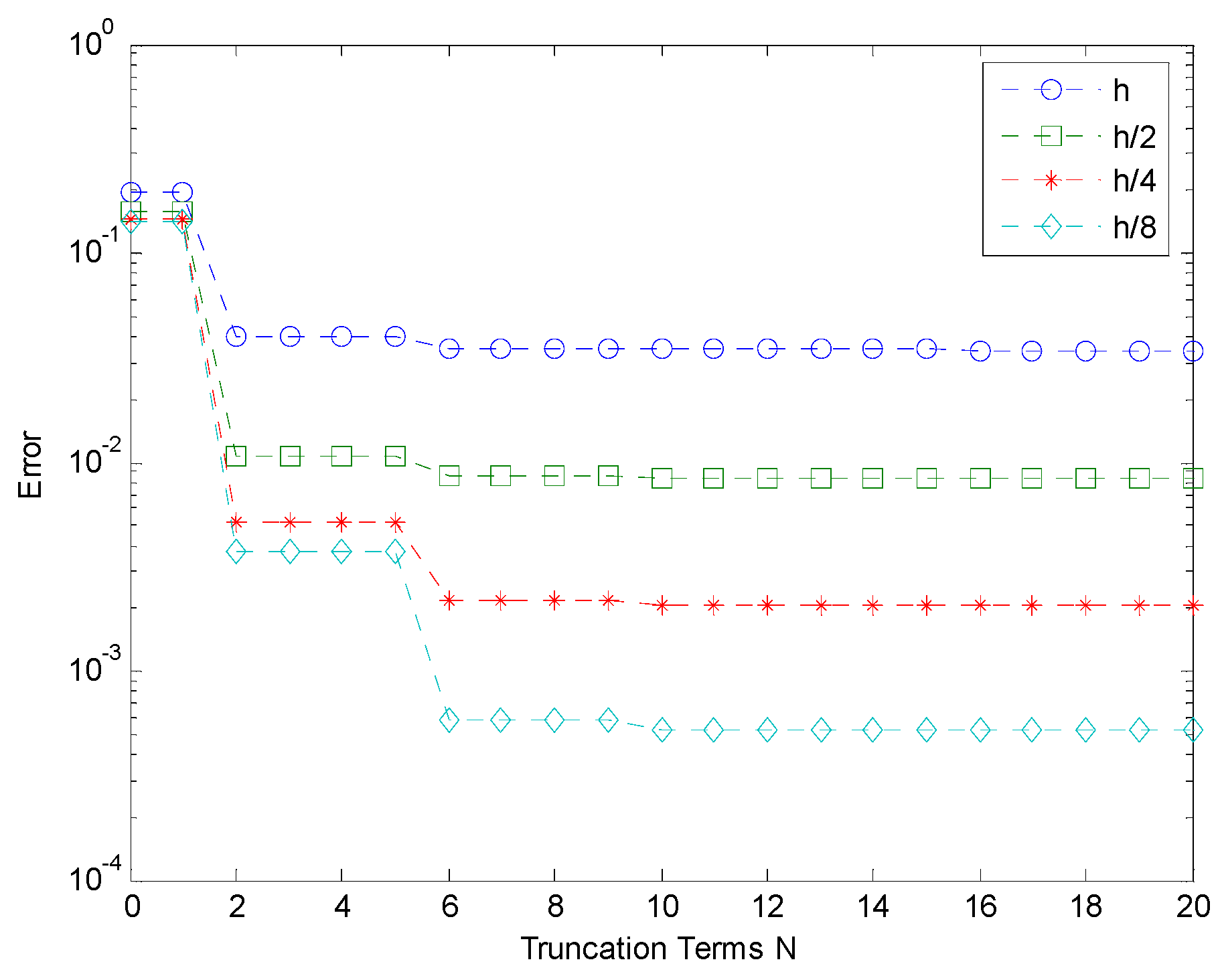
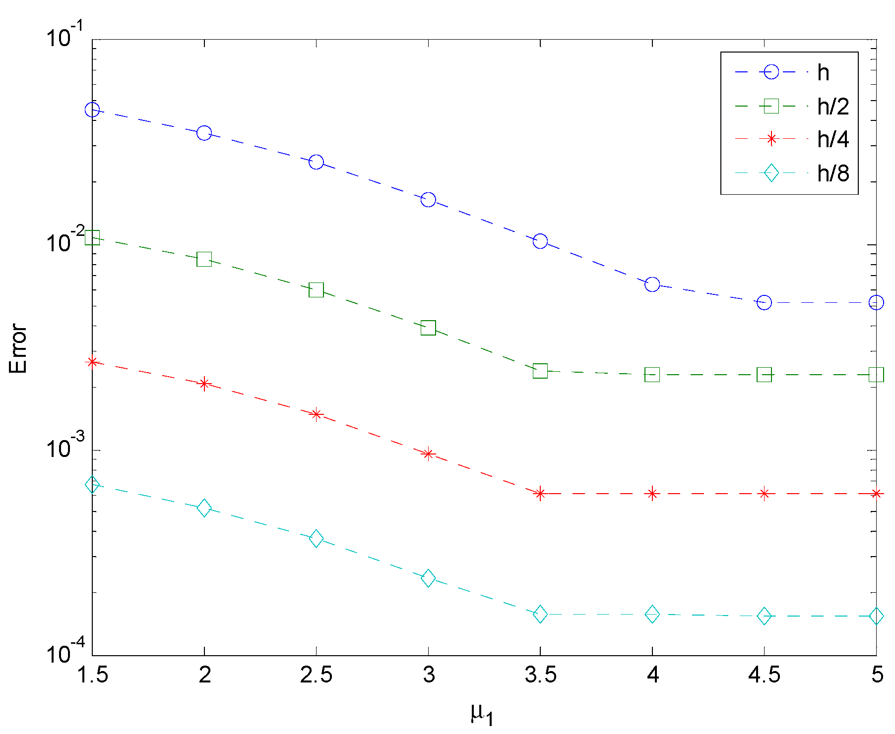
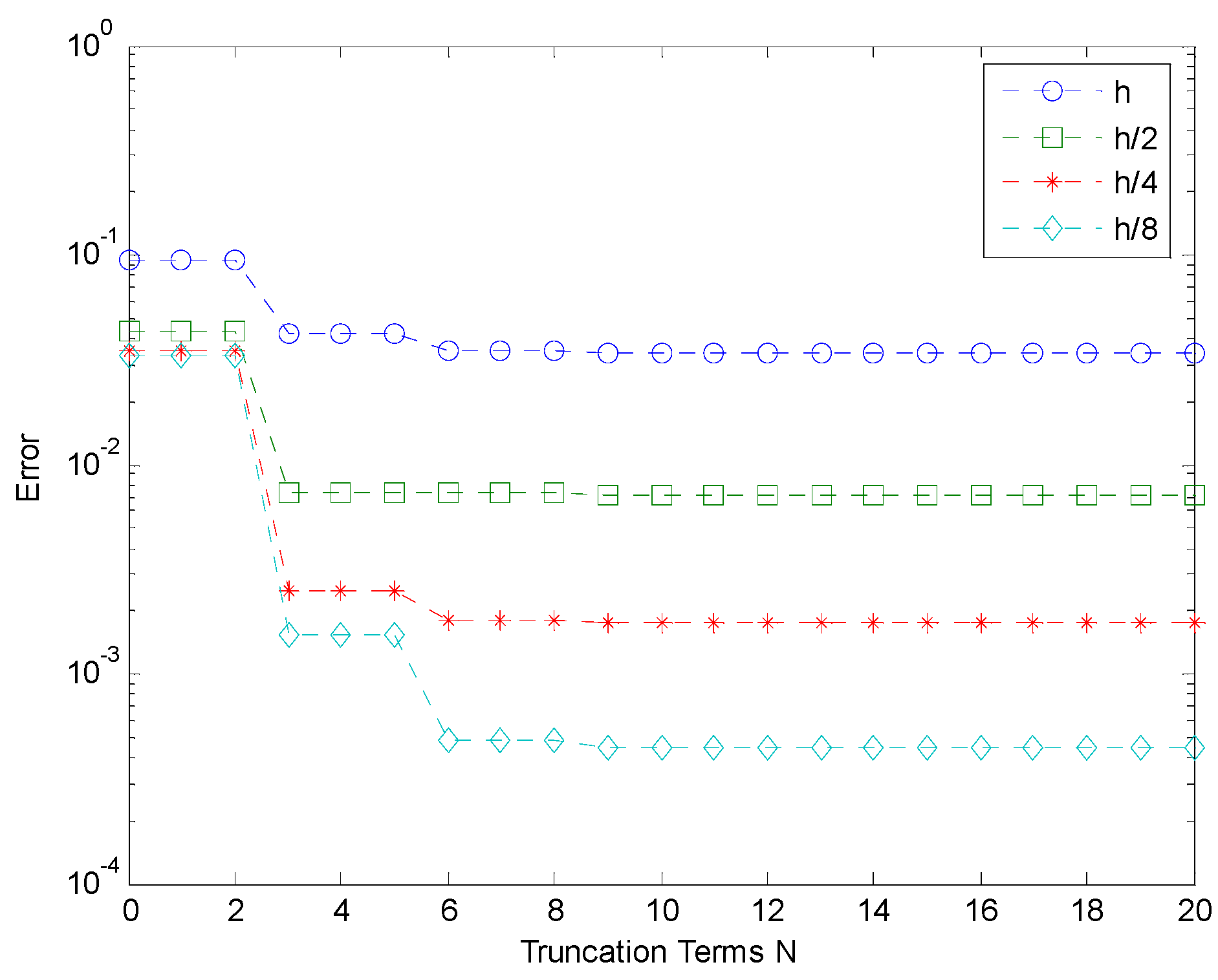
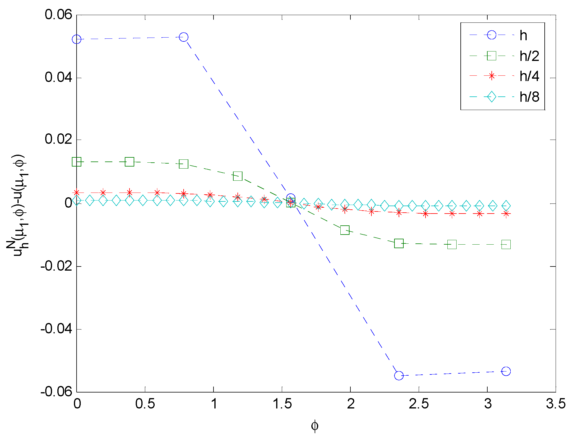
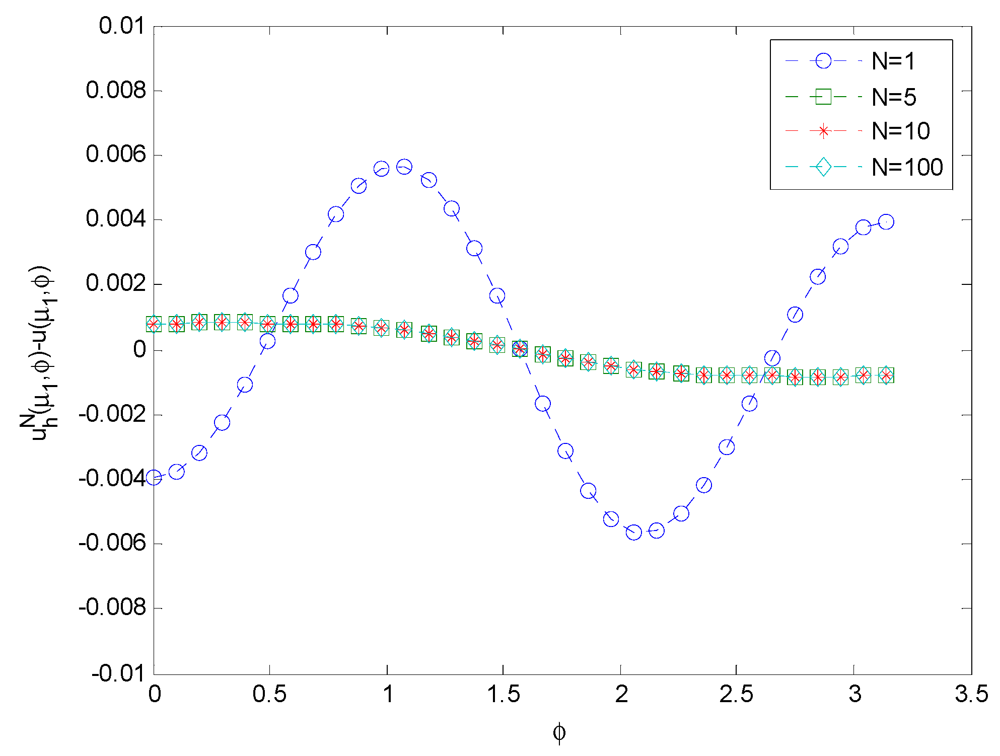
4. Numerical Examples

We computed three numerical examples using the method developed above to test the effectiveness of the method.

Example 1. 

We take $\Omega =\{\left(\mu ,\phi \right)|\mu >{\mu }_0, 0<\phi <2\pi \}$,$\Gamma =\left\{\left(\mu ,\phi \right)\right|\mu ={\mu }_0,0<\phi <2\pi \}$, ${\Gamma }_0=\left\{\left(\mu ,0\right)|\mu >{\mu }_0\right\}$, ${\Gamma }_{\alpha }=\left\{\left(\mu ,2\pi \right)|\mu >{\mu }_0\right\}$, ${\Gamma }_{{\mu }_1}=\{\left({\mu }_1,\phi \right)|{\mu }_1>{\mu }_0,0<\phi <2\pi \}$, $f_0=1.5$, ${\mu }_0=1$ and $a\left(x,u\right)=\frac{1}{1+u^2}$. The exact solution of original problem is $u=\tan \frac{2\cosh \mu \cos \phi }{f_0\left(\cosh 2\mu +\cos 2\phi \right)}$. Figure 3 shows Mesh $h$ of subdomain ${\Omega }_i \left({\mu }_1=2\right)$. The numerical results are given in

Table 1. The errors against mesh for Example 1 (μ₁ = 2, N = 20).

Mesh	$L^2\left({\Omega }_i\right)$ Error	$L^{\infty }\left({\Omega }_i\right)$ Error
$h$	0.078260	0.034508
$h/2$	0.015860	0.008414
$h/4$	0.003546	0.002088
$h/8$	0.000840	0.000521

, Figure 4 and Figure 5.

Example 2. 

We take $\Omega =\{\left(\mu ,\phi \right)|\mu >{\mu }_0, 0<\phi <\frac{3\pi }{2}\}$,$\Gamma =\left\{\left(\mu ,\phi \right)\right|\mu ={\mu }_0,0<\phi <\frac{3\pi }{2}\}$, ${\Gamma }_0=\left\{\left(\mu ,0\right)|\mu >{\mu }_0\right\}$, ${\Gamma }_{\alpha }=\left\{\left(\mu ,\frac{3\pi }{2}\right)|\mu >{\mu }_0\right\}$, ${\Gamma }_{{\mu }_1}=\{\left({\mu }_1,\phi \right)|{\mu }_1>{\mu }_0,0<\phi <\frac{3\pi }{2}\}$, $f_0=1.5$, ${\mu }_0=1$ and $a\left(x,u\right)=\frac{1}{\sqrt{1-u^2}}$. The exact solution of original problem is $u=\sin \frac{4\left({\cosh }^2\mu {\cos }^2\phi -{\sinh }^2\mu {\sin }^2\phi \right)}{f_0^2{\left(\cosh 2\mu +\cos 2\phi \right)}^2}$. Figure 6 shows Mesh $h$ of subdomain ${\Omega }_i \left({\mu }_1=2\right)$. The numerical results are given in

Table 2. The errors against mesh for Example 2 $\left({\mu }_1=2,N=20\right)$.

Mesh	$L^2\left({\Omega }_i\right)$ Error	$L^{\infty }\left({\Omega }_i\right)$ Error
h	0.064870	0.033738
h/2	0.011609	0.007163
h/4	0.002651	0.001776
h/8	0.000636	0.000444

, Figure 7 and Figure 8.

Example 3. 

We take $\Omega =\left\{\left(x,y\right)|x^2+2y^2>2, y>0\right\}$,$\Gamma =\left\{\left(x,y\right)|x^2+2y^2=2,y>0\right\}=\left\{\left(\mu ,\varphi \right)\right|\mu ={\mu }_0, 0<\varphi <\pi \}$, where $f_0=1$ and ${\mu }_0=\ln \left(\sqrt{2}+1\right)$. ${\Gamma }_0=\left\{\left(x,0\right)|x>\sqrt{2}\right\}$, ${\Gamma }_{\alpha }=\left\{\left(x,0\right)\right|x<-\sqrt{2}\}$, ${\Gamma }_{{\mu }_1}=\left\{\left({\mu }_1,\varphi \right)\right|{\mu }_1=2,0<\varphi <\pi \}$ and

$$a\left(x,u\right)=\{\begin{array}{c}4-x^2-y^2+\frac{1}{\sqrt{1-u^2}}, 2\le x^2+2y^2\le 4,\\ \frac{1}{\sqrt{1-u^2}}, x^2+2y^2>4,\end{array}$$

$$f\left(x\right)=\{\begin{array}{c}\frac{4-x^2-y^2}{{\left(x^2+y^2\right)}^2}\sin \frac{x}{x^2+y^2}-\frac{2x}{x^2+y^2}\cos \frac{x}{x^2+y^2}, 2\le x^2+2y^2\le 4,\\ 0, x^2+2y^2>4.\end{array}$$

The exact solution of original problem is $u=\sin \frac{x}{x^2+y^2}$. Figure 9 shows Mesh $h$ of subdomain ${\Omega }_i$. The numerical results are given in

Table 3. The errors against mesh for Example 3 $\left(N=10\right)$.

Mesh	$L^2\left({\Omega }_i\right)$ Error	$L^{\infty }\left({\Omega }_i\right)$ Error
$h$	0.091740	0.054584
$h/2$	0.018287	0.013246
$h/4$	0.004044	0.003287
$h/8$	0.000950	0.000820

, Figure 10 and Figure 11.

The numerical experiments show that the errors can be reduced by refining the finite element mesh, increasing the order of the artificial boundary condition or enlarging the location of the artificial boundary. Numerical experiments are identical with the theoretical analysis and show that the proposed method is very effective.

5. Conclusions

In this paper, we propose an artificial boundary method using elliptical arc artificial boundary for exterior quasilinear problems in concave angle domains. Based on the Kirchhoff transformation, we obtain the exact and a series of approximate boundary conditions. We formulate the finite element approximation in a bounded region using the approximate elliptical arc artificial boundary condition. We also provide error estimates depend on the finite element mesh, the order of the artificial boundary condition and the location of artificial boundary. Our numerical examples show the efficiency of our method.

An elliptical arc artificial boundary is advantageous in that it may be used to enclose slender obstacles with a concave angle efficiently, so that only a small computational domain in the immediate vicinity of the obstacle is need. It is much better than the circular arc one since it does not increase the computational complexity of the stiff matrix from artificial boundary. Using the elliptical arc boundary condition we proposed in this paper, one can design other numerical methods, for example, the non-overlapping and overlapping domain decomposition methods to solve the exterior quasilinear problems in concave angle domains. The results in this paper extend many related results about the numerical methods for quasilinear problems in unbounded domains.

References

1. Han, H.; Wu, X. Approximation of infinite boundary condition and its application to finite element methods. J. Comput. Math. 1985, 3, 179–192. [Google Scholar]
2. Han, H.; Wu, X. The Artificial Boundary Method—Numerical Solutions of Partial Differential Equations on Unbounded Domains; Tsinghua University Press: Beijing, China, 2009. [Google Scholar]
3. Feng, K. Finite element method and natural boundary reduction. In Proceedings of International Congress Mathematicians; Polish Academy Press: Warszawa, Poland, 1983. [Google Scholar]
4. Feng, K.; Yu, D. Canonical integral equations of elliptic boundary value problems and their numerical solutions. In Proceedings of China-France Symposium on the Finite Element Methods; Science Press: Beijing, China, 1983. [Google Scholar]
5. Yu, D. Natural Boundary Integral Method and Its Applications; Kluwer Academic Publishers: Amsterdam, The Netherlands, 2002. [Google Scholar]
6. Keller, J.B.; Givoli, D. Exact non-reflecting boundary conditions. J. Comput. Phys. 1989, 82, 172–192. [Google Scholar] [CrossRef]
7. Grote, M.J.; Keller, J.B. On non-reflecting boundary conditions. J. Comput. Phys. 1995, 122, 231–243. [Google Scholar] [CrossRef] [Green Version]
8. Hlavacek, I.; Krizek, M.; Maly, J. On Galerkin approximations of a quasi-linear nonpotential elliptic problem of a nonmonotone type. J. Math. Anal. Appl. 1994, 184, 168–189. [Google Scholar] [CrossRef] [Green Version]
9. Hlavacek, I. A note on the Neumann problem for a quasilinear elliptic problem of a nonmonotone type. J. Math. Anal. Appl. 1997, 211, 365–369. [Google Scholar] [CrossRef] [Green Version]
10. Chow, S. Finite element error estimates for non-linear elliptic equations of monotone type. Numer. Math. 1989, 54, 373–393. [Google Scholar] [CrossRef]
11. Liu, W. Finite element approximations of a nonlinear elliptic equation arising from biomaterial problems in elastic-plastic mechanics. Numer. Math. 2000, 86, 491–506. [Google Scholar] [CrossRef]
12. Korotov, S.; Křížek, M. Finite element analysis of varitional crimes for a quasilinear elliptic problem in 3D. Numer. Math. 2000, 84, 549–576. [Google Scholar] [CrossRef]
13. Milner, F.A. Mixed finite element methods for quasilinear second-order elliptic problems. Math. Comput. 1985, 44, 303–320. [Google Scholar] [CrossRef]
14. Meddahi, S. On a mixed finite element formulation of a second-order quasilinear problem in the plane. Numer. Methods Part. Differ. Equ. 2004, 20, 90–103. [Google Scholar] [CrossRef]
15. Karchevsky, M.; Fedotov, A. Error estimates and iterative procedure for mixed finite element solution of second-order quasi-linear elliptic problems. Comput. Methods Appl. Math. 2004, 4, 445–463. [Google Scholar] [CrossRef]
16. Houston, P.; Robson, J.; Suli, E. Discontinuous Galerkin finite element approximation of quasilinear elliptic boundary value problems I: The scalar case. IMA J. Numer. Anal. 2005, 25, 726–749. [Google Scholar] [CrossRef]
17. Houston, P.; Suli, E.; Wihler, T.P. A posteriori error analysis of hp-version discontinuous Galerkin finite-element methods for second-order quasi-linear elliptic PDEs. IMA J. Numer. Anal. 2008, 28, 245–273. [Google Scholar] [CrossRef]
18. Bi, C.; Ginting, V. A posteriori error estimates of discontinuous Galerkin method for nonmonotone quasi-linear elliptic problems. J. Sci. Comput. 2013, 55, 659–687. [Google Scholar] [CrossRef]
19. Sun, S.; Huang, Z.; Wang, C. Weak galerkin finite element method for a class of quasilinear elliptic problems. Appl. Math. Lett. 2018, 79, 67–72. [Google Scholar] [CrossRef]
20. Garau, E.M.; Morin, P.; Zuppa, C. Convergence of an adaptive Kačanov FEM for quasi-linear problems. Appl. Numer. Math. 2011, 61, 512–529. [Google Scholar] [CrossRef]
21. Guo, L.; Bi, C. Adaptive finite element method for nonmonotone quasi-linear elliptic problems. Comput. Math. Appl. 2021, 93, 94–105. [Google Scholar] [CrossRef]
22. Han, H.; Huang, Z.; Yin, D. Exact artificial boundary conditions for quasilinear elliptic equations in unbounded domains. Commun. Math. Sci. 2008, 6, 71–83. [Google Scholar] [CrossRef] [Green Version]
23. Liu, D.; Yu, D. A FEM-BEM formulation for an exterior quasilinear elliptic problem in the plane. J. Comput. Math. 2008, 26, 378–389. [Google Scholar]
24. Liu, B.; Du, Q. On the coupled of NBEM and FEM for an anisotropic quasilinear problem in elongated domains. Am. J. Comput. Math. 2012, 2, 143–155. [Google Scholar] [CrossRef] [Green Version]
25. Liu, B.; Du, Q. The Coupling of NBEM and FEM for quasilinear problems in a bounded or unbounded domain with a concave angle. J. Comput. Math. 2013, 31, 308–325. [Google Scholar]
26. Ingham, D.B.; Kelmanson, M.A. Boundary Integral Equation Analyses of Singular, Potential, and Biharmonic Problems; Springer: Beilin/Heidelberg, Germany, 1984. [Google Scholar]
27. Chen, Y.; Du, Q. Solution of exterior problems using elliptical arc artificial boundary. Eng. Lett. 2016, 24, 202–206. [Google Scholar]
28. Chen, C.; Zhou, J. Boundary Element Methods; Academic Press: London, UK, 1992. [Google Scholar]
29. Meddahi, S.; Gonzalez, M.; Perez, P. On a FEM-BEM formulation for an exterior quasilinear problem in the plane. SIAM J. Numer. Anal. 2000, 37, 1820–1837. [Google Scholar] [CrossRef] [Green Version]
30. Xu, J. Theory of Multilevel Methods. Ph.D. Thesis, Cornell University, Ithaca, NY, USA, 1989. [Google Scholar]
Figure 1. The illustration of domain Ω.
Mathematics 09 01598 g001
Figure 2. Two different artificial boundaries: (a) The circular arc artificial boundary Γ R ; (b) The elliptical arc artificial boundary Γ μ 1 .
Mathematics 09 01598 g002
Figure 3. Mesh h of Ω i for Example 1.
Mathematics 09 01598 g003
Figure 4. L ( Ω i ) errors against N for Example 1 ( μ 1 = 2 ) .
Mathematics 09 01598 g004
Figure 5. L ( Ω i ) errors against μ 1 for Example 1 (N = 20).
Mathematics 09 01598 g005
Figure 6. Mesh h of Ω i for Example 2.
Mathematics 09 01598 g006
Figure 7. L ( Ω i ) errors against N for Example 2 ( μ 1 = 2 ) .
Mathematics 09 01598 g007
Figure 8. L ( Ω i ) errors against μ 1 for Example 2 ( N = 20 ) .
Mathematics 09 01598 g008
Figure 9. Mesh h of Ω i for Example 3.
Mathematics 09 01598 g009
Figure 10. The errors on the artificial boundary against mesh for Example 3 ( N = 10 ) .
Mathematics 09 01598 g010
Figure 11. The errors on the artificial boundary against N for Example 3 ( Mesh   h / 8 ) .
Mathematics 09 01598 g011