A Multi-Depot Vehicle Routing Problem with Stochastic Road Capacity and Reduced Two-Stage Stochastic Integer Linear Programming Models for Rollout Algorithm

Abstract

A matheuristic approach based on a reduced two-stage Stochastic Integer Linear Programming (SILP) model is presented. The proposed approach is suitable for obtaining a policy constructed dynamically on the go during the rollout algorithm. The rollout algorithm is part of the Approximate Dynamic Programming (ADP) lookahead solution approach for a Markov Decision Processes (MDP) framed Multi-Depot Dynamic Vehicle Routing Problem with Stochastic Road Capacity (MDDVRPSRC). First, a Deterministic Multi-Depot VRP with Road Capacity (D-MDVRPRC) is presented. Then an extension, MDVRPSRC-2S, is presented as an offline two-stage SILP model of the MDDVRPSRC. These models are validated using small simulated instances with CPLEX. Next, two reduced versions of the MDVRPSRC-2S model (MDVRPSRC-2S1 and MDVRPSRC-2S2) are derived. They have a specific task in routing: replenishment and delivering supplies. These reduced models are to be utilised interchangeably depending on the capacity of the vehicle, and repeatedly during the execution of rollout in reinforcement learning. As a result, it is shown that a base policy consisting of an exact optimal decision at each decision epoch can be obtained constructively through these reduced two-stage stochastic integer linear programming models. The results obtained from the resulting rollout policy with CPLEX execution during rollout are also presented to validate the reduced model and the matheuristic algorithm. This approach is proposed as a simple implementation when performing rollout for the lookahead approach in ADP.

1. Introduction

Realistic modelling goes a long way in supporting effective relief operation in disasters. Such models allow uncertainties and dynamic updates with richer characteristics to be incorporated along with the model objectives. Most importantly, such models can be applied to various humanitarian operations during a disaster, such as the 2015 Nepal earthquake.

In this event, a 7.8 magnitude earthquake was registered, followed by several aftershocks resulting in the loss of roughly nine thousand lives. The remainder of the survivors were in dire need of relief aid [1] and were depending on the efficient delivery of relief supplies for their survival. Among the critical relief aid is medical supplies [2,3]. Adding to the challenges is the fact that Nepal is a landlocked country without any sea access, as the country is bordered by both China and India. As such, the only access to receive international aid is through the Tribhuvan Airport, which was flooded with relief aid. This caused a severe bottleneck, hampering efficient humanitarian operations [4]. On top of that, efficient relief operations were also hindered by landslides and tremors dismantling the transportation network, especially the access to remote places where medical supplies are scarce [5,6]. These challenges can be summarised as a bottleneck problem due to a single collection point and uncertainties in the road network, further constrained by limited transport vehicles. Multi-depots, instead of one single distribution point, could help alleviate the bottleneck problem. Limited vehicles could be made to perform split delivery and multi-trip operations as a means of compensating for the small number of vehicles available. After all, according to [7], 50% cost savings could be achieved through split delivery operations. In addition to the cost incurred by the operation, uncertainties in the road network had to be addressed and travel time was a concern. Given all these observations, the Multi-Depot Vehicle Routing Problem with Stochastic Road Capacity is proposed.

For this case, such a model is considered offline as defined by [8]. From the results presented in this paper, the offline computation gives a very optimistic solution given no dynamic elements are accounted for. For the online computation, changes towards parameters could be observed and re-computation can also be performed such that more accurate actions or decisions can be made efficiently and optimally, or at least close to optimality. An exact solution approach, such as the two-stage Stochastic Integer Linear Programming (SILP) model, is considered an offline computation approach. In this approach, an optimal route is computed prior to executing it in real life or real time. Alternatively, this exact approach could be used multiple times consecutively such that any new changes of parameter in real life could be adapted and re-computation could be conducted. Hence, the routing decision could be made in segments. For example, one may compute offline the whole route from the start of the mission to the end. However, one can also perform such computations at every node by making small adjustments to the previous parameters and constraints. Although this method is costly, as a complete route needs to be computed iteratively exactly, one can reduce the following model such that the computation would not be so punitive. A better reduction can lead to the separation of the goal of the reduced model after the initial computation is performed on the original main model. Furthermore, one may also incorporate the whole strategy within a larger solution framework such as Approximate Dynamic Programming (ADP) to allow for a more systematic update of the parameter at each decision point of time. This method is adopted in this work to incorporate dynamic elements of the problem, such as a deteriorating road capacity.

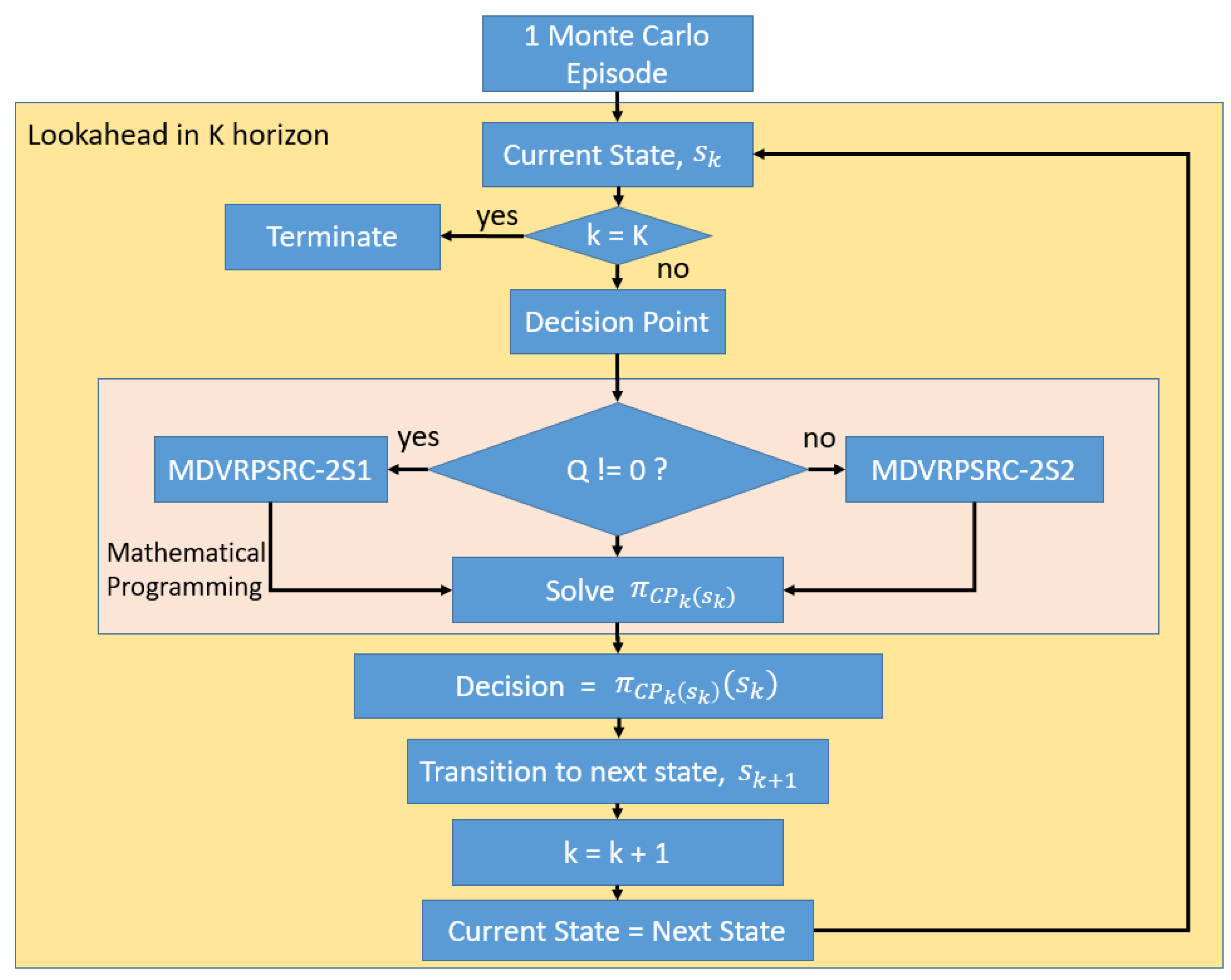
The curse of dimensionality [9] has been the moving factor in the development of ADP when solving the Bellman equation [10]. The key has always been about computing the values of the state $s_k$ in the vast explosion of state space $\mathbb{S}$ or the value of the action $a_k\in \mathbb{A}\left(s_k\right)$ given the state an agent is in. In ADP, these values are approximated to counter the curse of dimensionality. One of the non-parametric approaches of ADP includes the lookahead approach, which simulates the uncertain parameters through Monte Carlo simulation. The lookahead approach can be conducted through the rollout algorithm, where possible future events unfold from the point of decision onwards. The idea of a one step lookahead can be made analogous to a chess player that simulates a series of future events before making the best move. A two step lookahead would then mean that a chess player is thinking for two consecutive moves instead from the current state of the game. Any uncertain parameters are sampled instead via Monte Carlo simulation, typically based on a known stochastic distribution.

Besides uncertain parameter sampling, a future lookahead can only occur via a transitioning of states from the point of making decision $s_k$ onwards. This series of transitioning states is enabled by taking a set of actions according to a certain base policy throughout the lookahead. In a Vehicle Routing Problem (VRP), the base policy is the complete or partial route computed to allow the vehicle to perform humanitarian operations. This policy can be computed by using a construction heuristic, other specialised heuristics and even metaheuristics. Moreover, for cases of deterministic lookahead, an exact complete route could be computed through an Integer Linear Programming (ILP) approach.

In this study, the means to enable the computation of a base policy via an ILP approach for a Multi-Depot Dynamic Vehicle Routing Problem with Stochastic Road Capacity (MDDVRPSRC) dynamically is proposed by performing ILP iteratively at every decision point. Without such an approach, computing a complete route from the current state would lead to a non viable route as the road capacity might change when the next state is observed. This will prevent the vehicle from passing through certain roads on the pre-computed route. Here, the Deterministic Multi-Depot VRP with Road Capacity (D-MDVRPRC) and the two-stage Stochastic Integer Liner Programing (SILP) model, (MDVRPSRC-2S) for offline computation are presented and validated. The MDVRPSRC-2S is then reduced into two models that function separately based on the status of the operation for each vehicle: delivery (MDVRPSRC-2S1) or replenishment (MDVRPSRC-2S2). It is shown that these models could be used for MDDVRPSRC in the lookahead approach to construct the base policy on the go, while performing rollout. This is done by iteratively solving the reduced problem models.

The contribution of this paper is threefold. First, both deterministic and two-stage SILP models are presented along with two reduced models of the latter. Additionally, it is also shown that these models can be applied in the rollout setting. Next, it is also shown that the tremor progression of a disaster’s epicenter can be simulated, influencing the damage to the road network and thus the capacity of the road. Finally, the base policy for the rollout can be constructed dynamically on the go by solving the reduced models.

This paper is organised as follows: Section 2 describes the literature review focusing on the proposed models and rollout method in VRP. Section 3 describes the D-MDVRPRC and MDVRPSRC-2S problems, where the considerations for the time delay, road damage and random road capacity are elaborated. The two reduced models (MDVRPSRC-2S1 and MDVRPSRC-2S2) derived from MDVRPSRC-2S are presented in Section 4 with explanations of how they can be utilised in the rollout. Section 5 shows the numerical validation of D-MDVRPRC and MDVRPSRC-2S computed offline. MDVRPSRC-2S1 and MDVRPSRC-2S2 are validated through the rollout application and computational results are discussed. The research concludes in Section 6.

2. Literature Review

The MDVRPSRC describes the operation of split delivery throughout multi-trip operations from multi-depots while having to consider the stochastic road capacity within the network.

Different combinations and variations of these problem characteristics are especially addressed by the humanitarian operations applications. The review paper [11] had shown that those addressing split delivery VRP would also typically incorporate a multi-trip operation as a means to address the vehicle limitation problem during such a chaotic time. This could also be seen in [12,13,14,15,16]. Furthermore, a multi-depot problem is also adopted by several works to address a more realistic problem. Work that addresses both multi-depot and split delivery in the humanitarian operations setting can be found in [16,17,18]. As for works that addressed both multi-depot and multi-trip operations, this is seen in [19]. For a more in-depth, rich VRP that incorporates multi-depot, split delivery, multi-trip and road capacity for the application of humanitarian operations, refer to the work in [11].

Meanwhile, outside the field of humanitarian operations, the same trend could be observed where problem characteristics such as split delivery are usually addressed together with multi-trip operations [20]. In their work [20], the authors expand the Mixed Integer Linear Programming (MILP) model of VRP with multiple trips and split the delivery with time windows as well as heterogeneity of the vehicle fleet for optimised waste collection operations. A simple rule is applied to the heterogeneous vehicle fleet, where the largest vehicle should attend the largest collection point of waste.

In [21], similar considerations of split delivery, multiple trips and heterogeneous vehicles are addressed for the Fuel Replenishment Problem (FRP) with different types of fuel. The problem is formulated as an MILP model, where the solutions are compared with exact computations through a lower bound computed by column generation. Another FRP is addressed by [22], which considers split delivery, multiple trips, multi products and time windows as well as a heterogeneous fleet. The loads of vehicle and travel times are balanced and the model is solved with the sequential insertion heuristic methods. Ref. [23] resembles our proposed model the most, with the exclusion of road capacity consideration. Their work consists of solving problems involving split delivery and multi-trip as well as multi-depot operations for rice distribution among the poor using a homogeneous fleet of vehicles. Finally, [24] proposed an integer multi commodity flow model based on time network space planning for both the vehicle and product planning. Through this model, a split delivery, multi-trip and soft time windows problem is considered to replenish inventory in the supply chain. Other combinations of different problem characteristics could be observed from [25], which modeled a distribution problem considering multi-trip time windows as well as multi-products. Meanwhile, [26] addressed the usage of multi-depot to ease the travel times, multi-trip as well as time windows with a release date in the last mile of the distribution operation. In their work, [27] addressed the multi-trip with time windows for Pickup and Delivery VRP (PDVRP). Here, the roll containers are delivered while the emptied roll containers are collected according to the availability of the nurses in multiple hospitals as well as the work time of the drivers. This problem seeks to minimise the cost of travel as well as the usage of vehicles. This is solved using a Genetic Algorithm (GA) and the route-first cluster-second approach.

A standalone problem characteristic model can be seen in [28], which deals with delivery and packaging optimisation amidst the Corona Virus Disease (2019) (COVID-19). The proposed model addressed the difficulties of supply and demand while managing social isolation and movement control. Although the sole focus from the perspective of VRP is split delivery, an interesting consideration is given to reducing the number of split deliveries as to reduce the risk of infection by multiple contacts, in the event that a demand point hosted an infected person. Ref. [29] instead focused on the optimisation of production as well as delivery by incorporating the job scheduling problem and VRP into the proposed model. The VRP portion of the problem addresses the uncertain travel time where historical data might be lacking as well as multiple trips with time window operations. On the other hand, [30] proposed a split delivery VRP that aims to minimise the total distance travelled. For this problem, customers are separated into two groups depending on which is more suitable for a split delivery, which leads to an optimised route. In the humanitarian settings, more standalone problem characteristics of VRP in terms of split delivery, multi-trip and multi-depot can be observed in [11].

While still rarely addressed within the field of study, road capacity is highlighted in several works with deterministic and binary road capacity. Integer considerations, as well as deterministic to dynamic or stochastic road capacity, are also seen. In humanitarian operation settings, the characteristics of the road are a crucial factor albeit rarely addressed. As mentioned in [11] the flow model could be the best approach when incorporating road conditions such as road flow, road capacity and road impedance in a VRP. Such work can be seen in [31,32,33,34,35]. Moreover [36] associated road conditions by levels through circle-based areas of disaster from the point of disaster. Disaster affected roads are implied in [37] by restricting the number of vehicles on a specific arc through a constraint based on the travel time along the arc that is affected by disaster. On the other hand, [38,39] assumed a binary road capacity in their problem model. Uncertain road capacity is observed in [40]. Ref. [41] on the other hand implicitly incorporated road capacity by efficiently providing a rescue path during disaster through the three objectives that are optimised. Factors, such as the travel time and the reliability of the road, as well as the safety of the road, are optimised considering the road congestion and road capacity. Meanwhile, a crude binary form of road capacity is considered in [42]. In this particular problem, road capacity is rather exclusive to the type of vehicle used, namely vans and motorcycles for delivering goods. Narrow alleys are exclusive to motorcycles and some roads may prohibit the motorcycles but could be used by the vans. Through the model, the carbon emissions and the cost of replanning are reduced despite the addition of travel distance. All flow models utilised to describe a VRP often address road capacity either explicitly or implicitly. Ref. [43], for example, computes the optimal path for rescue emergency vehicles, taking into consideration the traffic congestion and the road capacity. Here, the road capacity is implicitly taken into consideration when the travel time and reliability of a path is computed and optimised. A dynamic road capacity is considered in [44] under the dynamic constraint for the flow of a vehicle and capacity of the road. This work addressed the flow of emergency materials problem where the decision of the dynamic origin of vehicles and the vehicle path are computed. In [45], the deterministic road capacity is incorporated within the lower level model to compute the time travel of a link. The optimised path consists of chosen links acting as the input to the upper model.

In terms of reflecting the damage on the road network due to the disaster, only the work of [36] can be considered. Here, the region of the network is superimposed on a circular region with the disaster point as the center. The outer ring network has less damage and thus less delay while the inner ring, which is closer to the disaster, suffered from more damage which would cause more delays. Our work differs from [36] as we denote the damage on each individual road based on the number of intersections of the circular radius dispersion from the epicenter of the earthquake. This circular radius dispersion is meant to represent the earthquake tremor radius through its wave-like motion and eruption. While a circular-based region might seem more natural to reflect the damage on the road network, ours has the ability to discern individual road damage (at the expense of computation time) should there be more than one epicenter, as was the case with the Nepal 2015 Earthquake.

The Reinforcement Learning (RL) adoption for stochastic VRP is seen in the work of [46], which provided the fundamentals or a framework for modelling a single stochastic VRP via Markov Decision Processes (MDP). This work is extended and modified by the same author in [47]. The former and latter are without computational results as the complex Operations Research problem then tends to prohibit an exact solution through dynamic programming. This necessitates the ADP approach for solving it. The need to approximate stems from the curse of dimensionality that plagues the framework of RL or Neuro Dynamic Programming (NDP) [48,49]. Among the ADP approaches is the lookahead approach for approximating the value of states rather than approximating the function for the value function itself. The rollout algorithm is one of the lookahead approaches proposed by [48], applied as part of the policy iteration scheme. In RL application for Operations Research, such a method was used from as early as 1998, where [50] developed a rollout algorithm specialised for sequencing problems and also for single VRP [51]. Furthermore, [49] compared the policy obtained from two policy iteration approaches, namely the optimistic approximate policy iteration and rollout policy where the latter outperformed the former for the single VRP. In [52], the rollout with a cyclic heuristic is applied for the application of the Travelling Salesman Problem with stochastic travel time and single VRP with Stochastic Demand.

Ref. [53] presented both the two-stage stochastic programming approach and the RL approach to solve for the single VRP with Stochastic Demand, the same as in [51]. However, [54] applied the Monte Carlo simulation instead of going through all the outcome spaces when performing the single stage and two-stage rollout, respectively. Such methods reduce computation by up to 65% as compared to [51]. Furthermore, [54] investigated a different approach with different base policies and different methods for estimating the value of state.

Ref. [55] eventually emerged with a multi-vehicle VRP with Stochastic Demand by employing the strategy in clustering the customers first for each respective vehicle. A deterministic a priori solution is computed for each vehicle for their respective customers. Should a failure occur, re-optimising through rollout is achieved due to the smaller partitioned customer nodes. Ref. [56] extends the idea by introducing a dynamic decomposition mechanism that adapts the clusters at each decision point in the Dynamic and Stochastic VRP for the problem of VRP with Stochastic Demand and Duration Limit. Furthermore, [56] proposed families of rollout algorithms including post decision rollout and pre decision rollout as well as hybrid rollout based on the extension of the MDP framework. The rollouts stem from the pre and post decision states as advocated by [57] to tackle the curse of dimensionality for larger and practical instances. Ref. [58] then went on to extend the work by addressing the problem of pre-emptive replenishment where the fixed route heuristic is adapted into a restocking fixed route heuristic. This was assisted by dynamic programming in evaluating the iterated policies within the local search process. Using this computed policy, the rollout is performed producing restocking-based rollout policies for the problem of VRP with Stochastic Demand and Duration Limit with pre-emptive replenishment. The same idea of applying dynamic programming to evaluating policies or routes computed by heuristics is highlighted by [59] for a single VRP with Stochastic Demand with restocking, this time with the hybrid of backward and forward recursion dynamic programming.

The first to deviate from the stochastic demand problem is [60], which addressed the VRP with stochastic customer requests, albeit only for a single vehicle. The post decision rollout algorithm is applied via the cheapest insertion heuristic and the result is compared using a value function approximation method as well as a greedy heuristic. This was later combined with the offline ADP through Value Function Approximation (VFA) and the online lookahead with Post Decision Rollout (PDS-RA) in [61]. Here, the VFA lookup table, which incorporates the temporal aspect of a customer request as state variables, forms a base policy to execute rollout that looks ahead through the transition of a detailed state that includes the spatial aspect of a customer request. Thus, both the temporal and spatial aspect of a stochastic customer request is addressed.

Finally, we direct the readers to [62,63,64], who made use of mathematical programming to obtain a base policy for the rollout of the problem involving a scheduling or inventory routing problem. For the scheduling problem, [64] applied a deterministic quadratic programming solution approach to obtain a feasible base heuristic for the rollout in solving the constrained MDP model. Meanwhile, [62] made use of an MILP rather than any heuristic to obtain a base policy for the rollout trajectories in order to estimate the value of the possible next state such that the rollout policy could be obtained for the single vehicle inventory routing problem. The same approach is applied in [63,65].

Although we too include the mathematical programming approach within the rollout structure, we differ from the previous mentioned works by constructing the base policy iteratively and dynamically using mathematical programming for every transition within the horizon of rollout. This resulted in a complete base policy for every rollout episode. To the best of our knowledge, such a method has not been published within the scholarly field.

3. Multi-Depot Vehicle Routing Problem with Stochastic Road Capacity

3.1. Problem Description

In the event of an earthquake, such as those in 2015 in Nepal, emergency shelters are set up at strategic locations to accommodate as many victims who are seeking medical help as possible.

To assist in the humanitarian logistic operations of medical supply delivery, homogeneous capacitated transport vehicles must travel from their respective depots to these emergency shelters to deliver medical supplies. Each of them are assigned to deliver medical supplies to these shelters and travels through connecting nodes and return back to any depot (not necessarily the depot from which it departed from).

During this operation, a vehicle is allowed to visit both the node and shelter as many times as possible if it is more efficient to do so. Emergency shelters that have been satisfied may serve as connecting nodes for vehicles to pass, en-route, to perform its task. Split delivery and multiple trips are allowed in order to satisfy all demands given the limited numbers of vehicles.

The decision maker must also take into account the road capacity along the routes that lead to the emergency shelters. These road capacities depend on whether the respective road is a highway, city road or a normal road. Thus the number of vehicles passing a road must be limited to that road capacity. Each road capacity within the network is stochastic, following the Poisson distribution representing the uncertain condition of the road when the disaster strikes. Moreover, each road’s capacity varies over the distribution whose mean value reflects the damage sustained by the road respectively. These damages are reflected by the intersection of an earthquake radial tremor circle and the road.

Each distance covered along the roads is proportional to the cost of the operation which is to be minimised so that the saved cost could be allocated to other critical humanitarian aid supplies. Additionally, the time travel along the road has an additional delay time depending on the damage sustained by the road.

The objective is to minimise the total travel time as well as the distance which represents the cost. Here, it is assumed that the highway road has the highest capacity, followed by the normal road and finally the city road in general. However, this is assuming no damage has been sustained by these roads. Otherwise, the capacity would reflect the damage sustained accordingly. Additionally, all vehicles are assumed to be travelling at a constant speed of 90 km per hour or per 60 min. From this assumption, the time travel or the delayed time travelled $T_{i,j}$ is computed. Finally, it is also assumed that the sampled road capacities and delayed time travel remained at the same value (non dynamic) despite multiple trips for offline computation. The problem is modelled as an undirected, incomplete graph $GG=(N,E)$. For both D-MDVRPRC and MDVRPSRC-2S, the parameters and variables are presented in

Table 1. Parameters and Variables for D-MDVRPRC and MDVRPSRC-2S.

Parameters
N	connecting node set
D	depot set
S	shelter set
H	$N\bigcup S\bigcup D$
E	set of edges $E=\left\{\right(i,j):i,j\in N\bigcup S\bigcup D,i\ne j\}$
$w_i$	demand of emergency shelter i
M	set of vehicles
G	set of trips
U	order index of edge $(i,j)$ in a route
Q	maximum capacity of vehicles after replenishment at depot
$C_{i,j}$	cost incurred if edge $(i,j)$ is travelled
$T_{i,j}$	time travelled of edge $(i,j)$
$r_{i,j}$	deterministic road capacity $r_{i,j}\in {\mathbb{Z}}^{🟉}$, where $Z^{🟉}={\mathbb{Z}}^{+}\bigcup \left\{0\right\}$
$\widehat{r_{i,j}}$	stochastic road capacity $\widehat{r_{i,j}}\in {\mathbb{Z}}^{🟉}$
Z	random event set where $Z=\{0,1\}=\{z_0,z_1\}$: $z_0\to \widehat{r_{i,j}}=0$ and $z_1\to \widehat{r_{i,j}}>0$
$\Omega$	penalty incurred when staying at current node $\left(i\right)$ due to random event $z_0$
$P_z$	Probability of edge $(i,j)$ with random event z
Variables
$x_{i,j,u,m,g}$	1, if vehicle m travel the edge $(i,j)\in E$ in the order of u in a route of trip $g\in G$
	0, otherwise
$q_{i,m,g}$	quantity served where $q_{i,m,g}\in {\mathbb{Z}}^{🟉}$ at shelter i by vehicle m on the trip g
$y_{i,j,u,m,g,z}$	1, if m stays at i on trip g due to $z_0$
	0, otherwise

.

3.2. Deterministic Integer Linear Programming Model (D-MDVRPRC)

In the deterministic model, the road capacity is deterministic. However, the road capacity is subjected to damages sustained by the road. Furthermore, the travel time along the damaged road is extended, representing difficulties when travelling along the damaged road.

The index u is introduced to represent the consecutive order of edges travelled, forming a route in trip g such that any nodes in the network could be visited many times while ignoring the subtour restriction.

The objective is to minimise the total travel cost and total travel time:

$$\begin{array}{c}\hfill {\displaystyle min\sum _{(i,j)\in E}\sum _{u\in U}\sum _{m\in M}\sum _{g\in G}{x}_{i,j,u,m,g}{C}_{i,j}+x_{i,j,u,m,g}{T}_{i,j}.}\end{array}$$

(1)

The constraints are formulated as follows:

$$\begin{array}{c}\hfill {\displaystyle \sum _{i\in D}\sum _{j\in S\bigcup N}{x}_{i,j,0,m,g}=1\forall m\in M,\forall g\in G,}\end{array}$$

(2)

with Constraint (2) ensuring one vehicle m departs only from one depot to other destinations for every one trip, if more than one trip is involved.

$$\begin{array}{c}\hfill {\displaystyle \sum _{i\in S\bigcup N}\sum _{j\in D}\sum _{u\in U}{x}_{i,j,u,m,g}\le 1\forall m\in M,\forall g\in G.}\end{array}$$

(3)

Constraint (3) ensures vehicle m returns to only (any) one depot for every one trip, if more than one trip is involved.

$$\begin{array}{c}\hfill {\displaystyle \sum _{i\in S\bigcup N\bigcup D}{x}_{i,j,u,m,g}-\sum _{i\in S\bigcup N\bigcup D}{x}_{j,i,u+1,m,g}=0\forall j\in S\bigcup N,\forall u\in U,\forall m\in M,\forall g\in G.}\end{array}$$

(4)

Constraint (4) ensures the vehicle that reaches a node, besides a depot, also comes out from that node (flow conservation).

$$\begin{array}{c}\hfill {\displaystyle \sum _{m\in M}{x}_{i,j,u,m,g}\le r_{i,j}\forall (i,j)\in E,\forall u\in U,\forall g\in G.}\end{array}$$

(5)

Constraint (5) is the road capacity constraint, which should be valid for each one of the trips g, not the collective of all trips.

Additionally, constraints (6)–(8) are adopted from [66] to expand the delivery among shelters in $\left|G\right|$ trips. With this formulation, the split delivery is also addressed:

$$\begin{array}{c}\hfill {\displaystyle \sum _{m\in M}\sum _{g\in G}{q}_{i,m,g}=w_i\forall i\in S.}\end{array}$$

(6)

Constraint (6) ensures that the demand at each of the shelters is satisfied through the course of all trips.

$$\begin{array}{c}\hfill {\displaystyle \sum _{i\in S}{q}_{i,m,g}\le Q\forall m\in M,\forall g\in G.}\end{array}$$

(7)

Constraint (7) states that each vehicle can only deliver its maximum capacity Q during one trip.

$$\begin{array}{c}\hfill {\displaystyle \left(\sum _{u\in U}\sum _{i\in H}{x}_{i,j,u,m,g}·Q\right)-q_{j,m,g}\ge 0\forall j\in S,\forall m\in M,\forall g\in G.}\end{array}$$

(8)

Constraint (8) links the routing decision variable to the quantity served decision variable with the possibility of multiple visits to one shelter in one trip, if it is optimal to do so.

$$\begin{array}{c}\hfill {\displaystyle \sum _{i\in D}\sum _{j\in N}{x}_{i,j,1,m,g}=0\forall m\in M,\forall g\in G.}\end{array}$$

(9)

Meanwhile, Constraint (9) prevents a premature return to the depot in case the shelter is not one step away from the depot.

$$\begin{array}{c}\hfill {\displaystyle \sum _{u\in U}{x}_{i,j,u,m,g}=1\forall (i,j)\in E,\forall m\in M,\forall g\in G.}\end{array}$$

(10)

Furthermore, Constraint (10) ensures only one variable $x_{i,j,u,m,g}$ would carry the value of one at a specific order u. Lastly, Constraints (10) and (11) ensure that a vehicle can serve as many shelters provided that it does not violate its maximum capacity when departing from a depot at each trip. This also leads to the following trips (after the first trip) utilizing just enough vehicles to serve the remaining demands.

$$\begin{array}{c}\hfill {\displaystyle \sum _{i\in D}\sum _{j\in (N+S)}{x}_{i,j,0,m,g}·Q-\sum _{i\in S}{q}_{i,m,g}\ge 0\forall m\in M,\forall g\in G.}\end{array}$$

(11)

3.3. Time Delay and Damage Determination

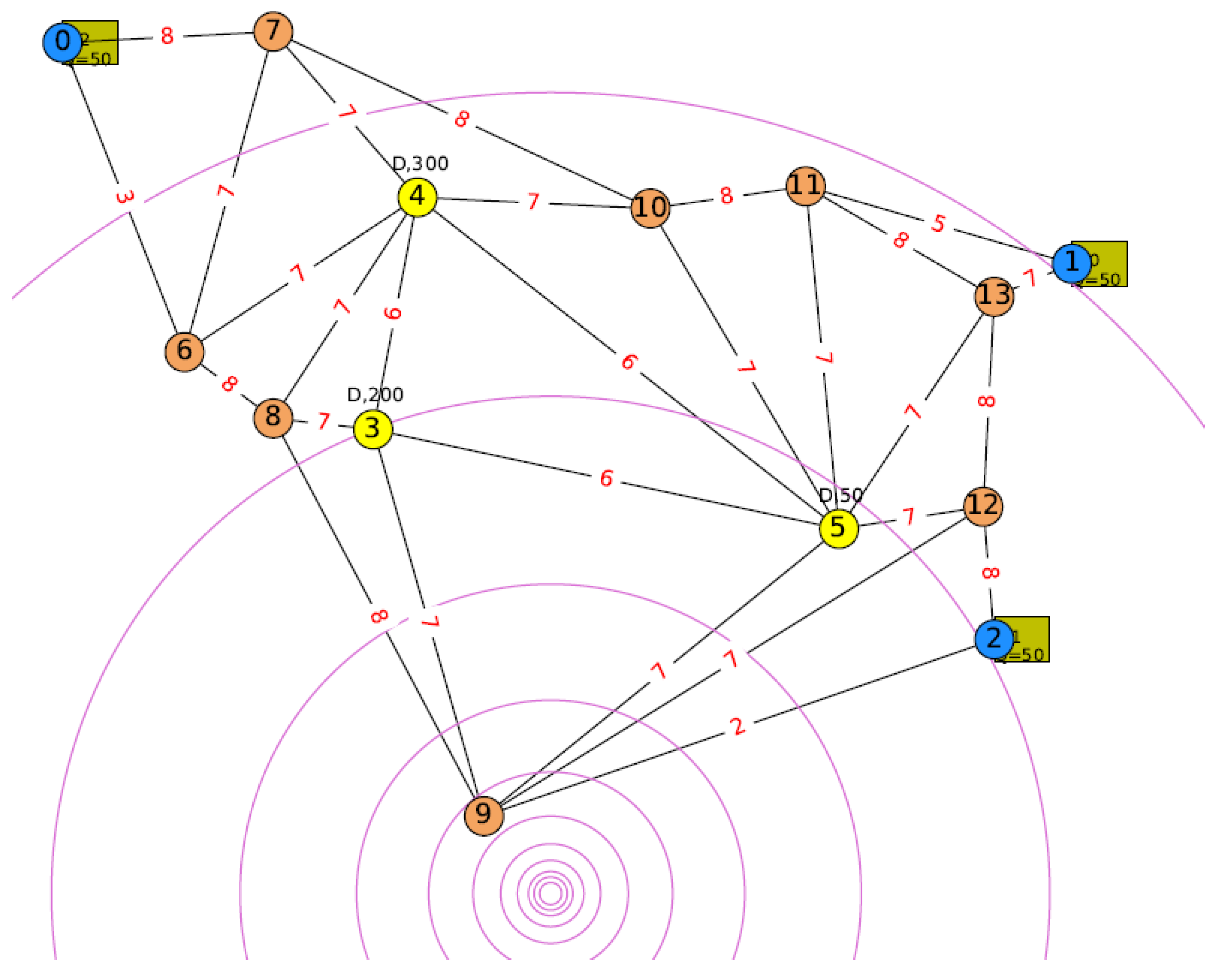
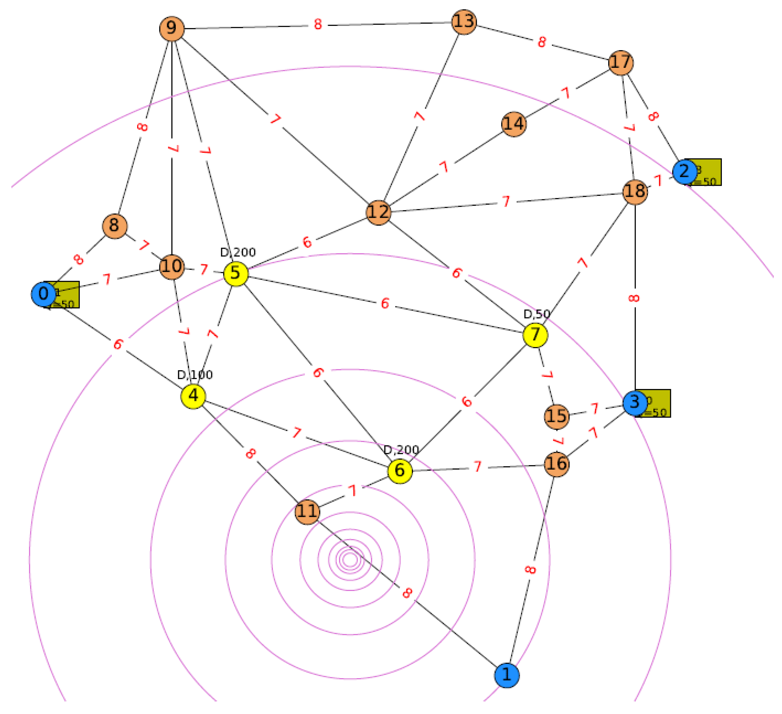
The delayed travel time for travelling along a damaged road or edge is determined based on the damage sustained by the road $(i,j)$. The damage sustained by an edge or road on the other hand is determined by the interception of the radial circle of an earthquake tremor and the edge. For example, an edge $(i,j)$, having a damage of $p_{i,j}=4$, would have four interceptions from the dispersion radial circle of different radius. Figure 1 illustrates the earthquake tremor radial dispersion originating from an epicenter affecting the road network based on the interceptions of the radial circle lines and the edges. Edge (9, 2), for example, sustained damage of $p_{9,2}=4$.

Algorithm 1 shows how the radial dispersion could be simulated using Fibonacci’s numbers.

Algorithm 1 Pseudocode for determining damages on all edges in road network instance.

Require: Instance files Ensure:$edges:damages\leftarrow$ sum of intensity or interception 1: create graph network $GG=(N,E)$ using Networkx library (Python): 2: add edges $(i,j)\in E$ to the network 3: extracting list undirected edges $(i,j)\in E$ from the $GG$ 4: Create even outward radial radius apart by 5 unit up to outermost node in $GG$ 5: extracting Fibonacci sequence up to max radius of tremor 6: propagation tremor’s radius = radius ∈ Fibonacci sequence ⊂ the radius list 7: initialise intensity list and damages dictionary 8: for line $i,j$ in undirected edges list E do 9:     reset intensity list 10:    for epicenter in list of selected epicenter in Online Python GUI do 11:         for radius ∈ radius propagation of earthquake do 12:            create 2D line between 2 nodes i and j of undirected line $(i,j)$ using sympify library 13:            create 2D circle line of radius using sympify library from epicenter 14:            Obtain list of intersection coordinates using sympify library Python 15:            intensity list ← length of list of intersection coordinates 16:         end for 17:     end for 18:     $p_{i,j}=$ sum(intensity list) 19:     $damages:\mathrm{line}i,j\leftarrow p_{i,j}$ 20: end for 21: return $damages$

As mentioned earlier, a constant speed 90 km/hour is assumed for all vehicles. Based on the distance, which gives the cost $C_{i,j}$, the time $T_{i,j}$ without considering damage, $p_{i,j}$ is computed in minutes as:

$$\begin{array}{c}\hfill T_{i,j}=\frac{C_{i,j}\times 60}{90}.\end{array}$$

(12)

For each edge $(i,j)\in E$ sustaining damages of $p_{i,j}$, the time is updated, with delay, as below:

$$\begin{array}{c}\hfill T_{i,j}=\left\{\begin{array}{cc}\frac{C_{i,j}\times 60}{90},\hfill & p_{i,j}=0\hfill \\ \hfill & .\hfill \\ \frac{C_{i,j}\times 60}{90}+\left(\frac{C_{i,j}\times 60}{90}\times \frac{p_{i,j}}{10}\right),\hfill & p_{i,j}\ne 0\hfill \end{array}\right.\end{array}$$

(13)

3.4. Two-Stage Stochastic Integer Linear Programming Model (MDVRPSRC-2S)

The deterministic problem model can be extended into a two-stage SILP model. The solution computed based on the two-stage SILP model would result in routes for all vehicles for all trips, along with a recourse decision should random event $z\in Z$ occur due to random road capacity $\widehat{r_{i,j}}$, $\forall (i,j)\in E$. Here, the variable $y_{i,j,u,m,g,z}$ is introduced as the recourse rule should a failure of a computed route occur due to road capacity $\widehat{r_{i,j}}=0$ for edge $(i,j)$ in the computed route.

Two random events are considered where $Z=\{0,1\}=\{z_0,z_1\}$, with $z_0\to r_{i,j}=0$ and $z_1\to r_{i,j}>0$. Here, the recourse rule is such that:

$$\begin{array}{c}\hfill y_{i,j,u,m,g,z}=\left\{\begin{array}{cc}1,\hfill & \mathrm{stay}\mathrm{at}i,\mathrm{if}z=z_0:r_{i,j}=0\hfill \\ 0,\hfill & \mathrm{otherwise}\mathrm{proceed}\mathrm{along}\mathrm{a}\mathrm{priori}\mathrm{route},\hfill \end{array}\right.\end{array}$$

(14)

where the variable addresses vehicle $m\in M$ journeying a computed route if it should stop at current nodes i in the event of z on the trip $g\in G$. For example, the route: (0–7–4–7–0) in Figure 1 for one trip is computed for vehicle m that is currently at a depot (node 0). This vehicle is assigned to serve node 4, which is the shelter. If random event $z_0$ occurred where $r_{0,7}=0$, a recourse rule would prevent m from moving. Instead, m remains at the depot (node 0). Otherwise, if $z_1$ is observed where $r_{0,7}>0$, m should proceed according to the pre computed route to node 7. Therefore, part of the solution computed by the two-stage programming would be as such: (0[0,7]–7[7,4]–4[4,7]–7[7,0]–0). Although such a rule is rather obvious, the aim is to compute the best route for all trips. This is done while taking into consideration the random events z (as is done in objective (15)) that might happen once the route is computed as well as incorporating the defined recourse rule $y_{i,j,u,m,g,z}$. The route computed by this approach is thus different than the route computed deterministically where logical rules or decisions could be applied later in real time practice when a route failure occurs.

Here, the objective is to minimise the total travel cost and total travel time, taking into consideration of the probability of event z and the recourse variable y:

$$\begin{array}{c}\hfill {\displaystyle min\sum _{(i,j)\in E}\sum _{u\in U}\sum _{g\in G}\sum _{m\in M}{x}_{i,j,u,m,g}{C}_{i,j}+x_{i,j,u,m,g}{T}_{i,j}+2\sum _{(i,j)\in E}\sum _{u\in U}\sum _{m\in M}\sum _{g\in G}\sum _{z\in Z}{P}_z{y}_{i,j,u,m,g,z}\Omega .}\end{array}$$

(15)

The Constraints (1)–(11) hold true for the two-stage SILP model except for Constraint (5). Furthermore, Constraint (16) links the recourse rule to the routing decision variable $x_{i,j,u,m,g}$ and the stochastic decision variable $y_{i,j,u,m,g,z}$. Here, if random event $z_0$ occurs, a recourse decision rule would dictate that vehicle m remains at i despite binary $x_{i,j,u,m,g}$ computed as “True”:

$$\begin{array}{c}\hfill x_{i,j,u,m,g}-y_{i,j,u,m,g,0}=0\forall i,j\in E,\forall u\in U,\forall m\in M,\forall g\in G.\end{array}$$

(16)

Meanwhile, Constraint (17) ensures that vehicle m proceeds with path $(i,j)$ for random event $z_1$:

$$\begin{array}{c}\hfill y_{i,j,u,m,g,1}=0\forall i,j\in E,\forall u\in U,\forall m\in M,\forall g\in G,\end{array}$$

(17)

and finally constraint (5) is adapted for random road capacity:

$$\begin{array}{c}\hfill {\displaystyle \sum _{m\in M}{x}_{i,j,u,m,g}\le \widehat{r_{i,j}}\forall (i,j)\in E,\forall u\in U,\forall g\in G.}\end{array}$$

(18)

3.5. Random Road Capacity

Among the many random distributions chosen, Poisson distribution suits the MDVRPSRC-2S well as it is applied for a discrete random distribution for online computation. The Poisson distribution denotes the probability distribution of a random value at a given interval that is given by Equation (19) as:

$$\begin{array}{c}\hfill P\left(x\right)=\frac{{\mu }^x\times e^{-\mu }}{x!}.\end{array}$$

(19)

The general formulation of Poisson distribution is adapted for the case of random road capacity $\widehat{r_{i,j}}$ in Equation (20):

$$\begin{array}{c}\hfill P\left(\widehat{r_{i,j}}\right)=\frac{{\mu }_{i,j,k}^{\widehat{r_{i,j}}}\times e^{-{\mu }_{i,j,k}}}{\widehat{r_{i,j}}!}.\end{array}$$

(20)

The updated random road capacity $\widehat{r_{i,j}}$ for all edges $(i,j)\in E$ is observed during the triggered event (for online computation, this is when any vehicle arrives at their destination). This updated random road capacity consists of all road capacities for each of the edges that are observed by the agent in the online simulation. These random road capacities are assumed to remain unchanged throughout the duration onwards until the next triggered event. For the offline computation, a suitable interval is chosen by considering when a delivery mission is normally executed in the aftermath of the earthquake disaster.

In the online computation, the applied duration in updating the random road capacities is the duration between two consecutive decision points $(T_k-T_{k-1})$. At both decision points, one or multiple vehicles first arrive at the destination that was previously assigned in decision point $(k-1)$.

Based on Equation (20), it is clear that the task is to find a suitable mean value ${\mu }_{i,j,k}$ in order to obtain the probabilities of the stochastic road capacity for all edges at time k. In this distribution model, a suitable mean value ${\mu }_{i,j,k}$ is the road capacity over an interval of time. ${\mu }_{i,j,k}$ is computed by considering the dynamic updated maximum road capacity of the said edge $(i,j)$, $r_{i,j,max,T_k}$ minus the deteriorating capacity of the road, (${\delta }_{i,j}$).

Given the severity of a disaster such as an earthquake, the road capacity tends to degrade over time for the online and dynamic cases. Taking that into consideration, the random Poisson distribution at time $T_k$ is said to have a mean road capacity ${\mu }_{i,j,k}$ of edge $(i,j)$ over the interval of $T_k-T_{k-1}$. In the offline computation case, such as the two-stage SILP approach, a suitable interval value is chosen and $T_k$ is considered as the time at which the road capacity is at its full capacity $r_{i,j,max}$. Mean road capacity ${\mu }_{i,j,k}$ is then computed as:

$$\begin{array}{c}\hfill {\mu }_{i,j,k}=r_{i,j,max,T_k}-{\delta }_{i,j,N},\end{array}$$

(21)

where the value of ${\delta }_{i,j,N}$ is a normalised value of ${\delta }_{i,j}$ in the range $[0,r_{i,j,max,T_k}]\in \mathbb{R}$.

Furthermore, the mean road capacity of an edge $(i,j),{\mu }_{i,j,k}$ computed in Equation (21) is also the maximum capacity of the edge when sampling is made at time $T_k$. This means an assumption is made that the edge has an average of the maximum road or edge capacity during the interval of $T_k-T_{k-1}$. Therefore, in the dynamic and online operation, the maximum road capacity in the next observation $k+1$ is updated in Equation (22). This is also the reason why the sampled random road capacity is bounded by the value of the average road capacity.

$$\begin{array}{c}\hfill r_{i,j,max,T_{k+1}}={\mu }_{i,j,k}.\end{array}$$

(22)

The random Poisson distribution mean ${\mu }_{i,j,k}$ is thus translated as the mean road capacity observed over the interval of $T_k-T_{k-1}$ at the time $T_k$, following the two assumptions of Poisson distribution:

• The mean does not change over observed duration $T_k-T_{k-1}$.
• The events remain independent of each other.

The value of ${\delta }_{i,j}$ is determined by the maximum road capacity of the edge at time $T_k$, a constant damage parameter from the interception of the edge and the radial line of tremor dispersion of the earthquake, $p_{i,j}$. This also includes the interval between the current decision point and previous decision point $T_k-T_{k-1}$. Here, ${\delta }_{i,j}$ is assumed to be proportional to the damage rate $p_{i,j}\in \mathbb{R}$:

$$\begin{array}{c}\hfill {\delta }_{i,j}\propto p_{i,j}.\end{array}$$

(23)

It makes sense to relate that the more damage an edge sustained, the more likely that the road capacity of the edges deteriorates from its maximum capacity.

At the same time, ${\delta }_{i,j}$ is proportional to the time interval between the current and previous decision points given as:

$$\begin{array}{c}\hfill {\delta }_{i,j}\propto (T_k-T_{k-1}).\end{array}$$

(24)

Equation (24) is proposed based on the assumption that should the interval between two decision points be fairly small, such as five minutes, it would not make sense that the road capacity would change so much from its previous road capacity. However, if the time interval is large, such as 100 min, it stands to reason that the road capacity might have reduced over time. As such, the relationship between ${\delta }_{i,j}$ and the damages of the respective edges $p_{i,j}$, as well as the interval, can be formulated as found in Equation (25):

$$\begin{array}{c}\hfill {\delta }_{i,j}\propto p_{i,j}\times (T_k-T_{k-1}),\end{array}$$

(25)

 or

$$\begin{array}{c}\hfill {\delta }_{i,j}=P\times \left(p_{i,j}\right)\times (T_k-T_{k-1}),\end{array}$$

(26)

where P is a constant. The value of ${\mu }_{i,j,k}$ in Equation (20) should remain a positive value within the capacity of the edges. Thus, the value of ${\delta }_{i,j}$ is normalised in range $(0,r_{i,j,max,T_k}]$. Furthermore, the value obtained in Equation (26) should be normalised, given by the general normalisation equation:

$$\begin{array}{cc}\hfill \mathrm{normalised}{\delta }_{i,j,N}=& \frac{{\delta }_{i,j}-\min \mathrm{range}}{{\delta }_{i,j,max}-{\delta }_{i,j,min}}\times (\max \mathrm{range}+\min \mathrm{range}),\hfill \end{array}$$

(27)

where both the minimum range and minimum value of ${\delta }_{i,j}$ are 0, and the maximum value of ${\delta }_{i,j}$ is given as:

$$\begin{array}{c}\hfill \begin{array}{cc}\hfill {\delta }_{i,j,\max }& =P\times p_{i,j,max}\times {(T_k-T_{k-1})}_{\max }\hfill \\ & =P\times \mathrm{maximum}\mathrm{number}\mathrm{of}\mathrm{intersections}\mathrm{in}\mathrm{dictionary}\times 2\hfill \\ & \times \left(\mathrm{maximum}\mathrm{value}\mathrm{of}\mathrm{time}\mathrm{matrix}\right),\hfill \end{array}\end{array}$$

(28)

where an extreme interval time assumes that the decision is next triggered after a vehicle arrives at the farthest destination. This is denoted by the maximum value in the time matrix. To account for any delay associated by the arrival time, the maximum value of the time matrix is multiplied by two.

Once the value of ${\mu }_{i,j,k}$ is obtained from Equation (21), the random stochastic road capacity $\widehat{r_{i,j}}$ can be computed using the numpy library in Python:

$$\widehat{r_{i,j}}=\mathrm{np.random.poisson}(\mathrm{mean}={\mu }_{i,j,k}).$$

Finally, the random road capacity is bounded by ${\mu }_{i,j,k}$ as the upper limit:

$$\begin{array}{c}\hfill \widehat{r_{i,j}}=\left\{\begin{array}{cc}\widehat{r_{i,j}},\hfill & \widehat{r_{i,j}}<{\mu }_{i,j,k}\hfill \\ {\mu }_{i,j,k},\hfill & \widehat{r_{i,j}}>{\mu }_{i,j,k}.\hfill \end{array}\right.\end{array}$$

4. Reduced Two-Stage Stochastic Integer Linear Programming Model for Rollout Algorithm

4.1. Online MDP MDDVRPSRC Lookahead Approach

In the online, stochastic and dynamic versions of the problem, the MDDVRPSRC is modelled in MDP with a PDS structure [57]. The ADP solution approach is adopted to compute for a near optimal policy. In this paper, the solution approach is briefly explained instead of the MDP model formulation as the MDP model is not the focus of this paper.

The stochastic and dynamic problems (formulated in MDP) seek an optimal policy ${\pi }^{🟉}$ that maximises the total rewards $R(s_k,A^{{\pi }^{🟉}}\left(s_k\right))$. The total rewards are obtained upon making a decision, starting from the initial state $s_0$ to the next state $s_1$ until the end state $s_K$. Based on the principle of optimality [10], a policy is optimal if the decision or action taken at every decision point is optimal ($a^{🟉}$) such that ${\pi }^{🟉}:s_k\to a_k^{🟉}$, where $a_k^{🟉}=A^{{\pi }^{🟉}}\left(s_k\right)$. The Bellman equation [10] can be rewritten such that $a^{🟉}$ is computed in Equation (29) as:

$$a_k^{🟉}=\underset{a_k\in A\left(s_k\right)}{arg\; max}(R(s_k,a_k)+{\lambda }^k\mathbb{E}\left\{V_{k+1}\left(s_{k+1}\right)\right\}),$$

(29)

where the conventional approach is to estimate the next state value in order to compute for the optimal decision or action as in Equation (30):

$$a_k^{🟉}=\underset{a_k\in A\left(s_k\right)}{arg\; max}(R(s_k,a_k)+{\lambda }^k\mathbb{E}\left\{\overline{V_{k+1}}\left(s_{k+1}\right)\right\}).$$

(30)

However, such an approach leads to the computation of expectation, where the outcome space needs to be included. By introducing the PDS structure [57], as in Equation (31):

$$V_k^{a_k}\left(s_k^{a_k}\right)=\mathbb{E}\left\{V_{k+1}\left(s_{k+1}\right)\right\},$$

(31)

the exhaustive computation can be reduced as in Equation (32):

$$a_k^{🟉}=\underset{a_k\in A\left(s_k\right)}{arg\; max}(R(s_k,a_k)+{\lambda }^k{V}_k^{a_k}\left(s_k^{a_k}\right)).$$

(32)

The task is then to first approximate the value of post decision state instead and then compute the optimal action as in Equation (33):

$$a_k^{🟉}=\underset{a_k\in A\left(s_k\right)}{arg\; max}(R(s_k,a_k)+{\lambda }^k\overline{V_k^{a_k}}\left(s_k^{a_k}\right)).$$

(33)

The approximated value of the post decision state seen in Equation (33) could be obtained through the averaged rollout return after the N number of the Monte Carlo simulation for each PDS following the basic pseudo Algorithm 2 (see [8]). Here, the expected rollout return $B({\pi }_{\mathcal{B}\left(s_k^{a_k}\right)},k+1,K)$ [67] is obtained per rollout episode until the end horizon K following a policy ${\pi }_{\mathcal{B}\left(s_k^{a_k}\right)}$, which is obtained by $\mathcal{B}$ given the current state $s_k$:

$$B({\pi }_{\mathcal{B}\left(s_k^{a_k}\right)},k+1,K)={\mathbb{E}}^{{\pi }_{\mathcal{B}\left(s_k^{a_k}\right)}}\left\{{\displaystyle \sum _{i=k+1}^{K-1}{\lambda }^{i-k+1}R(s_i,A^{{\pi }_{\mathcal{B}\left(s_{k+1}\right)}}\left(s_i\right))|s_k,a_k}\right\}.$$

In this approach, $\mathcal{B}$ is typically a heuristic. However, recent advancements of the rollout show that $\mathcal{B}$ could also be by any method to obtain policy ${\pi }_{\mathcal{B}\left(s_{k+1}\right)}$, including mathematical programming.

Algorithm 2 Compute $\overline{V_k^a}\left(s_k^a\right)$ (as shown in [8] based on PDS-RA proposed by [67])

Require:$s_k$, $\lambda$, $a_k$ Ensure:$\overline{V_k^a}\left(s_k^a\right)$ 1: Intialise $n,k,R(s_k,a_k),B^n$ 2: $s_k^{a_k}=S^{M,a}(s_k,a_k)$ 3: ${\pi }_{\mathcal{B}\left(s_k^a\right)}\leftarrow \mathcal{B}\left(s_k^{a_k}\right)$ 4: while$n\le N$do 5:     $s^a\leftarrow s_k^a$ 6:     while $k\ne K$ do 7:         $R(s_k,a_k)=R(s_k,a_k)+{\lambda }^{k}R(s_k,a_k)$ 8:         $s_k=S^{M,W}(s^a,W_{k+1}\left(\omega (k+1)\right))$ 9:         $a_k\leftarrow A^{{\pi }_{\mathcal{B}\left(s_k^a\right)}}\left(s_k\right)$ 10:        $s^a=S^{M,a}(s_k,a_k)$ 11:        $k=k+1$ 12:     end while 13:     ${\widehat{B}}^n({\pi }_{\mathcal{B}\left(s_k^a\right)},k+1,K)\leftarrow R(s_k,a_k)$ 14:     ${\overline{V_k^a}}^n\left(s_k^a\right)={\overline{V_k^a}}^{n-1}\left(s_k^a\right)+{\displaystyle \frac{1}{n}}\left({\widehat{B}}^n({\pi }_{\mathcal{B}\left(s_k^a\right)},k+1,K)-{\overline{V_k^a}}^{n-1}\left(s_k^a\right)\right)$ 15:     $n=n+1$ 16: end while 17: return ${\overline{V_k^a}}^N\left(s_k^a\right)$

In the online MDDVRPSRC, the decision $a_k$ is a vector in a decision space $A\left(s_k\right)$ at state $s_k$. The decision is to assign the next destination for all vehicles at every decision point k,

$$a_k=a\in H^{\left|M\right|}=[a_1,a_2,....a_{\left|M\right|}]\in A\left(s_k\right),$$

where $A\left(s_k\right)$ is defined as:

$$\begin{array}{cc}\hfill A\left(S_k\right)=\{& a_k\in H^{\left|M\right|}:\hfill \\ & a_m=j,\forall \{m\in M^{\prime }:i=l_m,j\ne i,r_{i,j}>0,w_j\ne 0,q_m\ne 0,j\in O_m:O_m=S\}\hfill \\ & a_m=j,\forall \{m\in M^{\prime }:i=l_m,j\ne i,r_{i,j}>0,\sum _{h\in H}{w}_h\ne 0,q_m\ne 0,j\in O_m:O_m=H\cap S\}\hfill \\ & a_m=j,\forall \{m\in M^{\prime }:i=l_m,j\ne i,r_{i,j}>0,\sum _{h\in H}{w}_h\ne 0,q_m=0,j\in O_m:O_m=D\}\hfill \\ & a_m=j,\forall \{m\in M^{\prime }:i=l_m,j\ne i,r_{i,j}>0,\sum _{h\in H}{w}_h\ne 0,q_m=0,j\in O_m:O_m=H\cap D\}\hfill \\ & a_m=j,\forall \{m\in M^{\prime }:i=l_m,j\ne i,r_{i,j}>0,\sum _{h\in H}{w}_h=0,i\notin D,j\in O_m:O_m=D\}\hfill \\ & a_m=i,\forall \{m\in M^{\prime }:i=l_m,j\ne i,r_{i,j}=0\forall (i,j)\in E,\sum _{h\in H}{w}_h\ne 0,q_m=0\}\hfill \\ & a_m=j,\forall \{m\in M^{\prime }:i=l_m,j=i,\sum _{h\in H}{w}_h=0,i\in D\}\hfill \\ & a_m=l_m,\forall \{m\in M\backslash M^{\prime },\}\hfill \\ & \}\hfill \end{array}$$

where $M^{\prime }$ is a set of arrived vehicles and $q_m$ is the dynamic capacity of vehicle m. Furthermore, $O_m$ is defined as the set of immediate locations a vehicle can go to next based on the road network. From this set, an optimal $\widetilde{a_m^{🟉}}$ is selected via computation as seen in Equation (34).

To solve Equation (33) however, the decision space $A\left(s_k\right)$ could be too large for obtaining good solution within reasonable computation efforts. We thus propose that for every decision point k:

$$a_k^{🟉}\approx \widetilde{a_k^{🟉}}\in H^{\left|M\right|}=[\widetilde{a_1^{🟉}},\widetilde{a_2^{🟉}},....\widetilde{a_{\left|M\right|}^{🟉}}]\forall k,$$

and thus for every k and for every vehicle $m\in M^{\prime }$:

$$\widetilde{a_m^{🟉}}=\underset{a_m\in O_m}{arg\; max}(R(s_k,a_m)+{\lambda }^k\overline{V_k^{a_m}}\left(s_k^{a_m}\right))\forall (k,m).$$

(34)

Although $\widetilde{a_m^{🟉}}$ is computed for each vehicle by performing the rollout, it is observed for a short horizon and moderate or small Monte Carlo simulations; this proposed approach yields good results for the MDDVRPSRC. This is seen in the online computation results presented in Section 5.

Furthermore, matheuristic is applied where the base policy ${\pi }_{\beta \left(s_k^a\right)}$ obtained is constructed on the go, based on the iterative computation of the reduced two-stage SILP problems (MDVRPSRC-2S1 and MDVRPSRC-2S1 in Section 4.2). As such, the proposed algorithm deviates from the PDS–RA algorithm in Algorithm 2 as illustrated in Algorithm 3. Algorithm 3 is then extended to Algorithm 4 to compute for $\widetilde{a_m^{🟉}}$.

Here, the base policy ${\pi }_{\beta \left(s_k^a\right)}$ is constructed on the go based on every first decision of the mathematical programming solution policy at the lookahead rollout decision time k, which is iterated over K decision points in one Monte Carlo episode. Ideally, the rollout would be performed to lookahead until the end decision point, which is the end horizon of the MDP problem. However, K in the rollout algorithm could mean any determined horizon as far as how one wished to lookahead in future subject to computation constraint. At every rollout decision point k, CPLEX is called in the Python program to compute ${\pi }_{C{P}_k\left(s_k\right)}$ given the rollout current state $s_k$ (Figure 2). The policy ${\pi }_{C{P}_k\left(s_k\right)}$ is simply a route with the goal to either replenish at a depot (MDVRPSRC-2S2) or to serve a shelter (MDVRPSRC-2S1) depending on the capacity of the vehicle in the rollout lookahead state $s_k$. Depending on the capacity of the vehicle, one of the two reduced two-stage SILP model is solved (Figure 2). The first decision within the computed policy is the action or decision for the lookahead rollout state at which CPLEX is executed for, ${\pi }_{C{P}_k}\left(s_k\right)$.

Randomly changing road capacity at every decision point may disrupt a route computed offline. Hence the policy computed by CPLEX could not be applied directly throughout the one episode rollout (${\pi }_{\beta \left(s_k^a\right)}\ne {\pi }_{C{P}_k\left(s_k\right)}$). Instead, the first decision of the policy ${\pi }_{C{P}_k\left(s_k\right)}$ is taken as part of the base policy for the lookahead state k. The process continues until horizon K where the base policy ${\pi }_{\beta \left(s_k^a\right)}$ would then be fully constructed for one Monte Carlo simulation episode. This lookahead simulated episode is constructed based on the policy computed on the go to transition to the next lookahead rollout state $s_{k+1}$ as well as by the sampled random information $W_{k+1}$ of episode n observed during the rollout decision point k which in this work is the road capacities: $\widehat{r_{i,j}},\forall (i,j)\in E\leftarrow W_{k+1}\left(n(k+1)\right)$. In Algorithms 2–4, the post decision state during lookahead episode $s^a$ is differentiated from $s_k^a$ to avoid confusion.

The post decision state value which the rollout is executed for in Equation (34), $V_k^{a_m}\left(s_k^{a_m}\right)$ is then approximated towards the end of Algorithm 3. For every potential decision $a_m\in O_m$, the respective post decision state value ${\overline{V_k^{a_m}}}^N\left(s_k^{a_m}\right)$ is computed from Algorithm 4 to solve Equation (34). This holds true for $|O_m|\ne 1$, otherwise the value of $\widetilde{a_m^{🟉}}$ is obvious. Based on the approximated post decision state value for every approximated $\widetilde{a_m^{🟉}}$ obtained in Algorithm 4, the optimal decision $a_k^{🟉}$ is then approximated and applied in the MDP at decision point k.

Algorithm 3 Rollout Algorithm to Compute $\overline{V_k^{a_m}}\left(s_k^{a_m}\right)$

Require:$s_k$, $\lambda$, $a_m$ Ensure:$\overline{V_k^{a_m}}\left(s_k^{a_m}\right)$ 1: Intialise $n,k,R(s_k,a_m),B^n$ 2: $s_k^{a_m}=S^{M,a}(s_k,a_m)$ 3: while$n\le N$do 4:     $s^a\leftarrow s_k^{a_m}$ 5:     while $k\ne K$ do 6:         $R(s_k,a_m)=R(s_k,a_m)+{\lambda }^{k}R(s_k,a_m)$ 7:         $s_k=S^{M,W}(s^a,W_{k+1}\left(n(k+1)\right))$ 8:         ${\pi }_{C{P}_k\left(s_k\right)}\leftarrow CPLE{X}_k\left(s_k\right)$ 9:         ${\pi }_{B_{s_k^a}}\left(s_k\right)\leftarrow {\pi }_{C{P}_k\left(s_k\right)}\left(s_k\right)$ 10:         $a_m\leftarrow A^{{\pi }_{\mathcal{B}\left(s_k^a\right)}}\left(s_k\right)$ 11:         $s^a=S^{M,a}(s_k,a_m)$ 12:         $k=k+1$ 13:     end while 14:     ${\widehat{B}}^n({\pi }_{\mathcal{B}\left(s_k^a\right)},k+1,K)\leftarrow R(s_k,a_m)$ 15:     ${\overline{V_k^{a_m}}}^n\left(s_k^{a_m}\right)={\overline{V_k^{a_m}}}^{n-1}\left(s_k^{a_m}\right)+{\displaystyle \frac{1}{n}}\left({\widehat{B}}^n({\pi }_{\mathcal{B}\left(s_k^a\right)},k+1,K)-{\overline{V_k^{a_m}}}^{n-1}\left(s_k^{a_m}\right)\right)$ 16:     $n=n+1$ 17: end while 18: return ${\overline{V_k^{a_m}}}^N\left(s_k^{a_m}\right)$

Algorithm 4 Extended from Algorithm 3 to Compute $\widetilde{a_m^{🟉}}$

Require:$s_k$, $\lambda$, $a_k$ Ensure:$a_m^{🟉}$ 1: for$a_m\in O_m$ at decision point k do 2:     Initialise $n,k,R(s_k,a_k),B^n$ 3:     while $n\le N$ do 4:         $s_k^{a_m}=S^{M,a}(s_k,a_m)$ 5:         $s^a\leftarrow s_k^{a_m}$ 6:         while $k\ne K$ do 7:            $R(s_k,a_m)=R(s_k,a_m)+{\lambda }^{k}R(s_k,a_m)$ 8:            $s_k=S^{M,W}(s^a,W_{k+1}\left(n(k+1)\right))$ 9:            ${\pi }_{C{P}_k\left(s_k\right)}\leftarrow CPLE{X}_k\left(s_k\right)$ 10:            ${\pi }_{B_{s_k^a}}\left(s_k\right)\leftarrow {\pi }_{C{P}_k\left(s_k\right)}\left(s_k\right)$ 11:            $a_m\leftarrow A^{{\pi }_{\mathcal{B}\left(s_k^a\right)}}\left(s_k\right)$ 12:            $s^a=S^{M,a}(s_k,a_m)$ 13:            $k=k+1$ 14:         end while 15:         ${\widehat{B}}^n({\pi }_{\mathcal{B}\left(s_k^a\right)},k+1,K)\leftarrow R(s_k,a_m)$ 16:         ${\overline{V_k^{a_m}}}^n\left(s_k^{a_m}\right)={\overline{V_k^{a_m}}}^{n-1}\left(s_k^{a_m}\right)+{\displaystyle \frac{1}{n}}\left({\widehat{B}}^n({\pi }_{\mathcal{B}\left(s_k^a\right)},k+1,K)-{\overline{V_k^{a_m}}}^{n-1}\left(s_k^{a_m}\right)\right)$ 17:         $n=n+1$ 18:     end while 19:     $f:{\overline{V_k^{a_m}}}^N\left(s_k^{a_m}\right)\to a_m$ 20: end for 21: $\widetilde{a_m^{🟉}}=\underset{a_m\in O_m}{arg\; max}f$ 22: return $\widetilde{a_m^{🟉}}$

4.2. Reduced Two-Stage Stochastic Integer Linear Programming Model

In order to execute CPLEX in the rollout algorithm iteratively with multiple Monte Carlo episodes and a suitable horizon of lookahead, the ILP model of the MDVRPSRC-2S needed to be substantially reduced. Since it is a lookahead approach, the setup of the problem should retain the same characteristics, such as the uncertain road capacity. However, the problem task is separated into two and reduced substantially due to the online solution that is required instead of the offline solution.

Since the rollout is executed only for a single vehicle, the problem in Section 3.4 is reduced to a single vehicle version of the problem. In this reduced version, the vehicle has only a single task, which is to either reach one emergency shelter (MDVRPSRC-2S1) and deliver the medical supply or to replenish its capacity if the total demand is still not fully satisfied (MDVRPSRC-2S2). These two tasks eliminate the requirement for both multi-trip and split delivery. Therefore, both the decision variable $q_{i,m,g}$ and parameter or index $g\in G$ are no longer required. Due to flexibility needed in reusing edges within a completed route, index u is still needed to arrange the edges forming the route and for allowing some subtour.

The same approach is taken when considering the random road capacities as well as their probability values from the random distribution as in Section 3.5. The online approach is taken where the interval is taken as the dynamic $T_k-T_{k-1}$. Therefore, the deterioration factor changes dynamically as in Equation (26). Furthermore, the mean ${\mu }_{i,j,k}$ of the distribution of all edges changes accordingly based on the dynamic maximum road capacity $r_{i,j,max,T_k}$ due to Equation (22). The road capacity observed at the point of decision in the lookahead episode n is: $\widehat{r_{i,j}}\forall (i,j)\in E\leftarrow W_{k+1}\left(n(k+1)\right)$, where $W_{k+1}$ is obtained from the random distribution. Finally, the time delay for a damaged road is considered as elaborated in Section 3.3.

For both MDVRPSRC-2S1 and MDVRPSRC-2S2, the parameters and variables in

Table 2. Parameters and Variables for MDVRPSRC-2S1 and MDVRPSRC-2S2.

Parameters
N	connecting nodes set
D	depot set
S	shelter set
$S^{\prime }$	unserved shelter set $S^{\prime }\subset S$
H	$N\bigcup S\bigcup D$
E	set of edges $E=\left\{\right(i,j):i,j\in N\bigcup S\bigcup D,i\ne j\}$
$w_i$	demand of emergency shelter i
M	set of vehicles
U	order index of edge $(i,j)$ in a route
$l_m$	current position of arrived vehicle m
Q	maximum capacity of vehicles after replenishment at depot
$C_{i,j}$	cost incurred if edge $(i,j)$ is travelled
$T_{i,j}$	time travelled of edge $(i,j)$
$\widehat{r_{i,j}}$	stochastic road capacity $\widehat{r_{i,j}}\in {\mathbb{Z}}^{🟉}$
Z	random event set where $Z=\{0,1\}=\{z_0,z_1\}$: $z_0\to \widehat{r_{i,j}}=0$ and $z_1\to \widehat{r_{i,j}}>0$
$\Omega$	penalty incurred when staying at current node $\left(i\right)$ due to $\widehat{r_{i,j}}=0$
$P_z$	Probability of edge $(i,j)$ with random event z
Variables
$x_{i,j,u,m}$	1, if vehicle m travel the edge $(i,j)\in E$ in the order of u in a route
	0, otherwise
$y_{i,j,u,m,z}$	1, if m stays at i due to $z_0$
	0, otherwise

are applied.

4.2.1. Model for Delivery (MDVRPSRC-2S1)

The model where the vehicle is en-route for delivery (if the vehicle capacity is not empty) will have the objective of minimising the total travel cost and total travel time, taking into consideration the probability of event z and the recourse variable y:

$$\begin{array}{c}\hfill {\displaystyle min\sum _{(i,j)\in E}\sum _{u\in U}\sum _{m\in M}{x}_{i,j,u,m}{C}_{i,j}+x_{i,j,u,m}{T}_{i,j}+2\sum _{(i,j)\in E}\sum _{u\in U}\sum _{m\in M}\sum _{z\in Z}{P}_z{y}_{i,j,u,m,z}\Omega .}\end{array}$$

(35)

$$\begin{array}{c}\hfill {\displaystyle \sum _{\begin{array}{c}j\ne l_m\\ j\in S\bigcup N\end{array}}{x}_{i,j,0,m}=1\forall m\in M,i=l_m,}\end{array}$$

(36)

Constraint (36) ensures only one vehicle m departs from its current location at decision point k. Vehicle m is not allowed to travel to depot since it still has capacity and there is still an unserved shelter.

$$\begin{array}{c}\hfill {\displaystyle \sum _{i\in S\bigcup N\bigcup D\bigcap S^{\prime }}\sum _{j\in S^{\prime }}\sum _{u\in U}{x}_{i,j,u,m}=1\forall m\in M.}\end{array}$$

(37)

Constraint (37) ensures one vehicle m arrives at an unserved shelter.

$$\begin{array}{c}\hfill {\displaystyle \sum _{i\in S\bigcup N\bigcup D\bigcap S^{\prime }}{x}_{i,j,u,m}-\sum _{i\in S\bigcup N}{x}_{j,i,u+1,m}=0\forall j\in S\bigcup N\bigcap S^{\prime },\forall u\in U,\forall m\in M.}\end{array}$$

(38)

Constraint (38) ensures the vehicle that reaches a node (besides any unserved shelters and depot) also comes out from that node (flow conservation).

$$\begin{array}{c}\hfill x_{i,j,u,m}-y_{i,j,u,m,0}=0\forall i,j\in E,\forall u\in U,\forall m\in M.\end{array}$$

(39)

Meanwhile Constraint (39) links the recourse variable to the decision variable x.

$$\begin{array}{c}\hfill y_{i,j,u,m,1}=0\forall i,j\in E,\forall u\in U,\forall m\in M\end{array}$$

(40)

and finally constraint (5) is adapted to form the random road capacity constraint (41):

$$\begin{array}{c}\hfill {\displaystyle \sum _{m\in M}{x}_{i,j,u,m}\le \widehat{r_{i,j}}\forall (i,j)\in E,\forall u\in U.}\end{array}$$

(41)

4.2.2. Model for Replenishment (MDVRPSRC-2S2)

This model has a vehicle en-route for replenishment (if the vehicle capacity empty) with the objective to minimise the total travel cost and total travel time, taking into consideration of the probability of event z and the recourse variable y:

$$\begin{array}{c}\hfill {\displaystyle min\sum _{(i,j)\in E}\sum _{u\in U}\sum _{m\in M}{x}_{i,j,u,m}{C}_{i,j}+x_{i,j,u,m}{T}_{i,j}+2\sum _{(i,j)\in E}\sum _{u\in U}\sum _{m\in M}\sum _{z\in Z}{P}_z{y}_{i,j,u,m,z}\Omega .}\end{array}$$

(42)

$$\begin{array}{c}\hfill {\displaystyle \sum _{\begin{array}{c}j\ne l_m\\ j\in S\bigcup N\bigcup D\end{array}}{x}_{i,j,0,m}=1\forall m\in M,i=l_m.}\end{array}$$

(43)

Constraint (43) ensures one vehicle m departs only from its current location at decision point k.

$$\begin{array}{c}\hfill {\displaystyle \sum _{i\in S\bigcup N}\sum _{j\in D}\sum _{u\in U}{x}_{i,j,u,m}=1\forall m\in M.}\end{array}$$

(44)

Constraint (44) ensures one vehicle m arrived at a depot.

$$\begin{array}{c}\hfill {\displaystyle \sum _{i\in S\bigcup N}{x}_{i,j,u,m}-\sum _{i\in S\bigcup N\bigcup D}{x}_{j,i,u+1,m}=0\forall j\in S\bigcup N\bigcap D,\forall u\in U,\forall m\in M.}\end{array}$$

(45)

Constraint (45) ensures the vehicle that reaches a node (besides depot) also comes out from that node (flow conservation). Furthermore, Constraints (39)–(41) are also applied for this model.

5. Computational Results and Discussions

The computational results obtained here are geared towards:

• The validation of the deterministic and stochastic (D-MDVRPRC and MDVRPSRC-2S) models;
• The validation and application of the reduced models (MDVRPSRC-2S1 and MDVRPSRC-2S2) in the MDDVRPSRC MDP model, and
• The application of the matheuristic proposed in the MDDVRPSRC.

While performing the validation test, comparative results are obtained between the proposed D-MDVRPRC and MDVRPSRC-2S models. To some degree, the offline and online computation are evaluated together. Where the online computation is concerned, the functionality of the reduced (MDVRPSRC-2S1 and MDVRPSRC-2S2) models applied in PDS–RA are shown. Since different behaviors of the vehicles are modelled in MDP, different results are to be expected.

The offline deterministic and stochastic models (D-MDVRPRC and MDVRPSRC-2S) are developed in Python 2.7 where CPLEX is executed through the DOCPLEX API for Python. Furthermore, the laptop computer used is running on Intel^R Core^TM i7-7500U CPU at 2.70–2.90 GHz with 20 GB RAM. In

Table 3. Parameter Configuration.

Parameter	Value
Deterioration Propotional Constant P	0.1
$\Omega$	200
Vehicle Speed	90 km/h
Vehicle Capacity, Q	50
Monte Carlo Simulation	3
Lookahead Horizon K	7

, the relevant parameters configured to run both the offline and online models are shown.

To illustrate the scenario of a disaster, the disaster in Nepal 2015 is referred to, and the simulated test instances are developed. The road network forms the undirected, incomplete graph. Since the purpose of the test is to validate a problem with a road capacity issue, typical benchmarks, such as Perl, Gaskell, and Christofides, are not considered suitable. Therefore, new simulated test instances are created to highlight some issues with the road capacities and the delivery process. Among the instances created, 18 were applied and the characteristics are shown in

Table 4. Parameter Configuration.

Instance	Depot	Shelter	Nodes	Vehicle	Total Demand	Road Capacity
D3N8S3_678_4	3	3	8	4	550	$6,7,8$
D3N8S3_678_8	3	3	8	8	550	$6,7,8$
D3N8S3_678_15	3	3	8	15	550	$6,7,8$
D3N8S3_234_4	3	3	8	4	550	$2,3,4$
D3N8S3_234_8	3	3	8	8	550	$2,3,4$
D3N8S3_234_15	3	3	8	15	550	$2,3,4$
D4N11S4_678_4	4	4	11	4	550	$6,7,8$
D4N11S4_678_8	4	4	11	8	550	$6,7,8$
D4N11S4_678_15	4	4	11	15	550	$6,7,8$
D4N11S4_234_4	4	4	11	4	550	$2,3,4$
D4N11S4_234_8	4	4	11	8	550	$2,3,4$
D4N11S4_234_15	4	4	11	15	550	$2,3,4$
D5N13S5_678_4	5	5	13	4	650	$6,7,8$
D5N13S5_678_8	5	5	13	8	650	$6,7,8$
D5N13S5_678_15	5	5	13	15	650	$6,7,8$
D5N13S5_234_4	5	5	13	4	650	$2,3,4$
D5N13S5_234_8	5	5	13	8	650	$2,3,4$
D5N13S5_234_15	5	5	13	15	650	$2,3,4$

.

More difficult instances are available for future work, which can be applied for online computation. Computation within reasonable time for both deterministic and stochastic model proved to be prohibitive for instance D6N16S6 (with 6 depots, 16 connecting nodes and 6 shelters) onwards. As such, only the results with listed instances are presented in this paper.

Three road networks that were tested can be seen in Figure A1, Figure A2 and Figure A3 with an epicenter of an earthquake roughly at the lower center part of all the road networks in the test instances (specific coordinates: (460, 180)). The blue, brown and yellow nodes are the depots, connecting nodes and emergency shelters respectively. The problem is modelled as the undirected, incomplete graph, where no node is completely connected to all other nodes and the distance is computed based on the Euclidean distance formulation. The number at the center of the edge represents the capacity of the road. The tuple $(6,7,8)$ represents the maximum road capacity of a highway city road, a normal road, and a highway respectively without taking the damage factor into consideration. A tighter maximum road capacity tuple $(2,3,4)$ is also introduced in some of the instances tested to study the difference in results as compared to the original maximum road capacity setting $(6,7,8)$. In the road network, the inner part edges are city roads while the outer part of the edges is the highway. In between the outer and inner regions are the normal roads. In the D-MDVRPRC model, the road capacity does not change after computing the maximum road capacity with respect to the damages at the initial stage. Meanwhile, in the MDVRPSRC-2S model, the capacity of the road is sampled randomly as described in Section 3.5 for offline computation. In the online simulation (rollout using MDVRPSRC-2S21 and MDVRPSRC-2S2), the road capacity changes, as can be seen in Figure A4 as compared to Figure A1. In Figure A4, it could be seen that shelters are all served and the vehicles are en-route back to the depot. At the simulated time (1152 min), which translated into an almost full day (19 hours and 12 min), the edges near the epicenter show a decrease in road capacity as compared to other edges although the setting for road capacity applied is $(6,7,8)$. In particular, edge $(9,2)$ or $(2,9)$ has zero capacity since the remaining capacity is used by the vehicles en-route to depot 2. Furthermore, the vehicle travelling along the damaged road experienced longer travel time than usual as described in Section 3.3. What can be also observed is that the road capacity of the edges, which experienced no damage (no interception on the edge), is still stochastic with the upper bound of the maximum computed road capacity. Finally, in all figures, the vehicle is denoted in either blue and green colors, differentiating the en-route vehicle and the arrived vehicle respectively with a capacity status shown within the square marker.

Based on these simulated test instances, the validation results for both the deterministic (D) and stochastic (S) MDVRPSRC-2S models are presented in

Table 5. Results of Total Distance Travelled with (Maximum) 15 Vehicles.

Instance	Mode	Mean (km)	Variance	Std. Dev. (km)	CV	Best (km)
D3N8S3_678_15	D	9099.94	0.00	0.00	0.00	9099.94
	S	9207.96	2.33 $\times {10}^4$	1.53 $\times {10}^2$	1.66 $\times {10}^{-2}$	9099.94
	SDY	22,530.46	2.73 $\times {10}^6$	1.65 $\times {10}^3$	7.33 $\times {10}^{-2}$	20,142.97
D3N8S3_234_15	D	9928.93	0.00	0.00	0.00	9928.93
	S	11,096.01	1.04 $\times {10}^5$	3.23 $\times {10}^2$	2.91 $\times {10}^{-2}$	10,696.04
	SDY	24,590.97	3.45 $\times {10}^6$	1.86 $\times {10}^3$	7.56 $\times {10}^{-2}$	21,910.79
D4N11S4_678_15	D	6601.66	0.00	0.00	0.00	6601.66
	S	6685.14	6.58 $\times {10}^3$	8.11 $\times {10}^1$	1.21 $\times {10}^{-2}$	6601.66
	SDY	16,682.46	3.92 $\times {10}^6$	1.98 $\times {10}^3$	1.19 $\times {10}^{-1}$	14,943.58
D4N11S4_234_15	D	6698.36	0.00	0.00	0.00	6698.36
	S	8090.86	5.67 $\times {10}^3$	7.53 $\times {10}^1$	0.93 $\times {10}^{-2}$	7993.87
	SDY	18,992.70	3.04 $\times {10}^6$	1.74 $\times {10}^3$	9.18 $\times {10}^{-2}$	17,426.28
D5N13S5_678_15	D	7406.06	0.00	0.00	0.00	7406.06
	S	7425.07	7.23 $\times {10}^2$	2.69 $\times {10}^1$	0.36 $\times {10}^{-2}$	7406.06
	SDY	23,777.44	1.34 $\times {10}^7$	3.66 $\times {10}^3$	1.54 $\times {10}^{-1}$	16,847.04
D5N13S5_234_15	D	7502.76	0.00	0.00	0.00	7502.76
	S	8098.67	1.50 $\times {10}^4$	1.23 $\times {10}^2$	1.51 $\times {10}^{-2}$	8010.88
	SDY	23,403.58	1.23 $\times {10}^7$	3.51 $\times {10}^3$	1.50 $\times {10}^{-1}$	17,486.9

,

Table 6. Results of Total Travel Time with (Maximum) 15 Vehicles.

Instance	Mode	Mean (min)	Variance	Std. Dev. (min)	CV	Best (min)
D3N8S3_678_15	D	707.36	0.00	0.00	0.00	707.36
	S	707.36	0.00	0.00	0.00	707.36
	SDY	1389.42	3.18 $\times {10}^4$	1.78 $\times {10}^2$	1.28 $\times {10}^{-1}$	1250.56
D3N8S3_234_15	D	834.20	0.00	0.00	0.00	834.20
	S	962.78	1.39 $\times {10}^4$	1.18 $\times {10}^2$	1.22 $\times {10}^{-1}$	845.40
	SDY	1583.61	2.15 $\times {10}^4$	1.47 $\times {10}^2$	9.26 $\times {10}^{-2}$	1322.54
D4N11S4_678_15	D	560.82	0.00	0.00	0.00	560.82
	S	568.96	1.33 $\times {10}^2$	1.15 $\times {10}^1$	2.02 $\times {10}^{-2}$	560.82
	SDY	1015.37	9.60 $\times {10}^3$	9.80 $\times {10}^1$	9.65 $\times {10}^{-2}$	932.44
D4N11S4_234_15	D	585.25	0.00	0.00	0.00	585.25
	S	803.45	7.54 $\times {10}^3$	8.69 $\times {10}^1$	1.08 $\times {10}^{-1}$	742.03
	SDY	1264.77	1.45 $\times {10}^4$	1.20 $\times {10}^2$	9.52 $\times {10}^{-2}$	1094.74
D5N13S5_678_15	D	560.82	0.00	0.00	0.00	560.82
	S	560.82	0.00	0.00	0.00	560.82
	SDY	1388.28	2.86 $\times {10}^4$	1.69 $\times {10}^2$	1.22 $\times {10}^{-1}$	1131.31
D5N13S5_234_15	D	585.25	0.00	0.00	0.00	585.25
	S	663.88	3.74 $\times {10}^3$	6.12 $\times {10}^1$	9.22 $\times {10}^{-2}$	585.25
	SDY	1456.50	3.68 $\times {10}^4$	1.92 $\times {10}^2$	1.32 $\times {10}^{-1}$	1131.31

,

Table 7. Results of Computation Time with (Maximum) 15 Vehicles.

Instance	Mode	Mean (s)	Variance	Std. Dev. (s)	CV	Best (s)
D3N8S3_678_15	D	7.07	2.14 $\times {10}^{-2}$	1.46 $\times {10}^{-1}$	2.07 $\times {10}^{-2}$	6.94
	S	17.12	1.26 $\times {10}^1$	3.55	2.07 $\times {10}^{-1}$	14.54
	SDY	1526.52	6.65 $\times {10}^4$	2.58 $\times {10}^2$	1.69 $\times {10}^{-1}$	1019.83
D3N8S3_234_15	D	138.57	3.02 $\times {10}^1$	5.49	3.96 $\times {10}^{-2}$	134.40
	S	244.79	1.50 $\times {10}^4$	1.23 $\times {10}^2$	5.01 $\times {10}^{-1}$	144.18
	SDY	1507.52	1.73 $\times {10}^5$	4.15 $\times {10}^2$	2.76 $\times {10}^{-1}$	942.88
D4N11S4_678_15	D	14.57	5.76 $\times {10}^{-1}$	7.59 $\times {10}^{-1}$	5.21 $\times {10}^{-2}$	13.57
	S	74.22	2.04 $\times {10}^3$	4.51 $\times {10}^1$	6.08 $\times {10}^{-1}$	41.97
	SDY	2031.02	6.39 $\times {10}^5$	8.00 $\times {10}^2$	3.94 $\times {10}^{-1}$	972.02
D4N11S4_234_15	D	65.01	3.36 $\times {10}^1$	5.79	8.91 $\times {10}^{-2}$	60.20
	S	396.72	1.33 $\times {10}^4$	1.15 $\times {10}^2$	2.91 $\times {10}^{-1}$	298.70
	SDY	1514.74	4.66 $\times {10}^4$	2.16 $\times {10}^2$	1.43 $\times {10}^{-1}$	1298.40
D5N13S5_678_15	D	118.52	5.4 $\times {10}^1$	7.35	6.20 $\times {10}^{-2}$	108.17
	S	116.47	8.08 $\times {10}^2$	2.84 $\times {10}^1$	2.44 $\times {10}^{-1}$	87.79
	SDY	4941.58	2.58$\times {10}^6$	1.61$\times {10}^3$	3.25$\times {10}^{-1}$	2826.50
D5N13S5_234_15	D	88.20	1.94	1.39	1.58 $\times {10}^{-2}$	86.25
	S	288.98	1.22 $\times {10}^4$	1.10 $\times {10}^2$	3.82 $\times {10}^{-1}$	133.09
	SDY	3146.13	4.42 $\times {10}^5$	6.65 $\times {10}^2$	2.11 $\times {10}^{-1}$	2414.39

,

Table 8. Results of Total Distance Travelled with (Maximum) 8 Vehicles.

Instance	Mode	Mean (km)	Variance	Std. Dev. (km)	CV	Best (km)
D3N8S3_678_8	D	9099.94	0.00	0.00	0.00	9099.94
	S	9099.94	0.00	0.00	0.00	9099.94
	SDY	19,573.79	4.88 $\times {10}^6$	2.21 $\times {10}^3$	1.13 $\times {10}^{-1}$	16,310.17
D3N8S3_234_8	D	9099.94	0.00	0.00	0.00	9099.94
	S	10,365.37	4.95 $\times {10}^5$	7.03 $\times {10}^2$	6.79 $\times {10}^{-2}$	9748.06
	SDY	19,965.72	2.55 $\times {10}^6$	1.60 $\times {10}^3$	8.01 $\times {10}^{-2}$	18,042.19
D4N11S4_678_8	D	6601.66	0.00	0.00	0.00	6601.66
	S	6601.66	0.00	0.00	0.00	6601.66
	SDY	12,769.48	2.90 $\times {10}^6$	1.70 $\times {10}^3$	1.33 $\times {10}^{-1}$	10,868.74
D4N11S4_234_8	D	6601.66	0.00	0.00	0.00	6601.66
	S	6704.15	6.30 $\times {10}^3$	7.94 $\times {10}^1$	1.18 $\times {10}^{-2}$	6601.66
	SDY	14,558.10	1.95 $\times {10}^6$	1.40 $\times {10}^3$	9.59 $\times {10}^{-2}$	12,502.33
D5N13S5_678_8	D	7406.06	0.00	0.00	0.00	7406.06
	S	7406.06	0.00	0.00	0.00	7406.06
	SDY	17,302.35	1.68 $\times {10}^6$	1.29 $\times {10}^3$	7.48 $\times {10}^{-2}$	14,553.92
D5N13S5_234_8	D	7406.06	0.00	0.00	0.00	7406.06
	S	7508.55	2.68 $\times {10}^2$	1.64 $\times {10}^1$	2.18 $\times {10}^{-3}$	7485.40
	SDY	18,303.25	3.71 $\times {10}^6$	1.93 $\times {10}^3$	1.05 $\times {10}^{-1}$	13,672.40

,

Table 9. Results of Total Travel Time with (Maximum) 8 Vehicles.

Instance	Mode	Mean (min)	Variance	Std. Dev. (min)	CV	Best (min)
D3N8S3_678_8	D	1252.17	0.00	0.00	0.00	1252.17
	S	1360.54	5.87 $\times {10}^3$	7.66 $\times {10}^1$	5.63 $\times {10}^{-2}$	1252.17
	SDY	1991.70	4.77 $\times {10}^4$	2.18 $\times {10}^2$	1.10 $\times {10}^{-1}$	1646.11
D3N8S3_234_8	D	1252.17	0.00	0.00	0.00	1252.17
	S	1448.22	3.24 $\times {10}^3$	5.69 $\times {10}^1$	3.93 $\times {10}^{-2}$	1401.54
	SDY	2108.74	3.86 $\times {10}^4$	1.96 $\times {10}^2$	9.31 $\times {10}^{-2}$	1889.42
D4N11S4_678_8	D	939.49	0.00	0.00	0.00	939.49
	S	922.90	5.51 $\times {10}^2$	2.35 $\times {10}^1$	2.54 $\times {10}^{-2}$	889.70
	SDY	1366.12	3.61 $\times {10}^4$	1.90 $\times {10}^2$	1.39 $\times {10}^{-1}$	1144.86
D4N11S4_234_8	D	939.49	0.00	0.00	0.00	939.49
	S	1025.55	4.62 $\times {10}^3$	6.79 $\times {10}^1$	6.62 $\times {10}^{-2}$	977.51
	SDY	1588.98	2.57 $\times {10}^4$	1.60 $\times {10}^2$	1.01 $\times {10}^{-1}$	1348.11
D5N13S5_678_8	D	939.49	0.00	0.00	0.00	939.49
	S	987.30	9.27 $\times {10}^3$	9.63 $\times {10}^1$	9.75 $\times {10}^{-2}$	900.76
	SDY	1796.10	1.90 $\times {10}^4$	1.38 $\times {10}^2$	7.68 $\times {10}^{-2}$	1528.07
D5N13S5_234_8	D	939.49	0.00	0.00	0.00	939.49
	S	1137.92	5.30 $\times {10}^2$	2.30 $\times {10}^1$	2.02 $\times {10}^{-2}$	1121.64
	SDY	1926.85	3.64 $\times {10}^4$	1.91 $\times {10}^2$	9.90 $\times {10}^{-2}$	1449.37

,

Table 10. Results of Computation Time with (Maximum) 8 Vehicles.

Instance	Mode	Mean (s)	Variance	Std. Dev. (s)	CV	Best (s)
D3N8S3_678_8	D	44.71	7.06	2.66	5.95 $\times {10}^{-2}$	42.62
	S	73.91	2.02 $\times {10}^3$	4.49 $\times {10}^1$	6.08 $\times {10}^{-1}$	34.48
	SDY	1199.77	1.15 $\times {10}^5$	3.39 $\times {10}^2$	2.82 $\times {10}^{-1}$	753.67
D3N8S3_234_8	D	57.10	8.54	2.92	5.12 $\times {10}^{-2}$	54.69
	S	1540.38	1.32 $\times {10}^6$	1.15 $\times {10}^3$	7.45 $\times {10}^{-1}$	144.20
	SDY	1200.27	9.80 $\times {10}^4$	3.13 $\times {10}^2$	2.61 $\times {10}^{-1}$	757.10
D4N11S4_678_8	D	22.90	1.81 $\times {10}^{-2}$	1.34 $\times {10}^{-1}$	5.87 $\times {10}^{-3}$	22.71
	S	133.84	1.55 $\times {10}^3$	3.94 $\times {10}^1$	2.95 $\times {10}^{-1}$	83.94
	SDY	1282.67	1.06 $\times {10}^5$	3.26 $\times {10}^2$	2.54 $\times {10}^{-1}$	802.23
D4N11S4_234_8	D	46.36	8.13 $\times {10}^{-1}$	9.02 $\times {10}^{-1}$	1.95 $\times {10}^{-2}$	45.44
	S	70.80	1.36 $\times {10}^3$	3.68 $\times {10}^1$	5.20 $\times {10}^{-1}$	42.03
	SDY	1094.18	1.25 $\times {10}^4$	1.12 $\times {10}^2$	1.02 $\times {10}^{-1}$	924.15
D5N13S5_678_8	D	190.92	2.21 $\times {10}^1$	4.70	2.46 $\times {10}^{-2}$	184.48
	S	240.57	1.83 $\times {10}^3$	4.27 $\times {10}^1$	1.78 $\times {10}^{-1}$	190.99
	SDY	3271.40	4.69 $\times {10}^5$	6.85 $\times {10}^2$	2.09 $\times {10}^{-1}$	2389.22
D5N13S5_234_8	D	190.12	6.82 $\times {10}^1$	8.26	4.34 $\times {10}^{-2}$	181.05
	S	202.44	5.63 $\times {10}^3$	7.51 $\times {10}^1$	3.71 $\times {10}^{-1}$	100.68
	SDY	3269.92	9.27 $\times {10}^5$	9.63 $\times {10}^2$	2.95 $\times {10}^{-1}$	2339.45

,

Table 11. Results of Total Distance Travelled with (Maximum) 4 Vehicles.

Instance	Mode	Mean (km)	Variance	Std. Dev. (km)	CV	Best (km)
D3N8S3_678_4	D	9099.94	0.00	0.00	0.00	9099.94
	S	9099.94	0.00	0.00	0.00	9099.94
	SDY	15,518.21	1.00 $\times {10}^6$	1.00 $\times {10}^3$	6.45 $\times {10}^{-2}$	14,336.66
D3N8S3_234_4	D	9099.94	0.00	0.00	0.00	9099.94
	S	9566.40	2.52 $\times {10}^5$	5.02 $\times {10}^2$	5.25 $\times {10}^{-2}$	9211.09
	SDY	15,397.60	4.87 $\times {10}^6$	2.21 $\times {10}^3$	14.3 $\times {10}^{-1}$	12,206.56
D4N11S4_678_4	D	6601.66	0.00	0.00	0.00	6601.66
	S	6620.67	7.23 $\times {10}^2$	2.69 $\times {10}^1$	4.06 $\times {10}^{-3}$	6601.66
	SDY	11,809.59	9.76 $\times {10}^5$	9.88 $\times {10}^2$	8.37 $\times {10}^{-2}$	10,039.78
D4N11S4_234_4	D	6601.66	0.00	0.00	0.00	6601.66
	S	6850.23	8.31 $\times {10}^4$	2.88 $\times {10}^2$	4.21 $\times {10}^{-2}$	6601.66
	SDY	12,169.90	1.25 $\times {10}^6$	1.12 $\times {10}^3$	9.18 $\times {10}^{-2}$	10,078.55
D5N13S5_678_4	D	7406.06	0.00	0.00	0.00	7406.06
	S	7406.06	0.00	0.00	0.00	7406.06
	SDY	12,751.34	1.14 $\times {10}^6$	1.07 $\times {10}^3$	8.36 $\times {10}^{-2}$	11,148.8
D5N13S5_234_15	D	7406.06	0.00	0.00	0.00	7406.06
	S	7849.32	1.08 $\times {10}^5$	3.28 $\times {10}^2$	4.18 $\times {10}^{-2}$	7406.06
	SDY	13,890.02	1.05	1.03 $\times {10}^3$	7.39 $\times {10}^{-2}$	12,206.56

,

Table 12. Results of Total Travel Time with (Maximum) 4 Vehicles.

Instance	Mode	Mean (min)	Variance	Std. Dev. (min)	CV	Best (min)
D3N8S3_678_4	D	1959.53	0.00	0.00	0.00	1959.53
	S	2067.91	5.87 $\times {10}^3$	7.66 $\times {10}^1$	3.71 $\times {10}^{-2}$	1959.53
	SDY	2965.15	6.25 $\times {10}^4$	2.50 $\times {10}^2$	8.43 $\times {10}^{-2}$	2592.54
D3N8S3_234_4	D	1959.53	0.00	0.00	0.00	1959.53
	S	1998.35	3.01 $\times {10}^3$	5.49 $\times {10}^1$	2.75 $\times {10}^{-2}$	1959.53
	SDY	2943.891	1.92 $\times {10}^5$	4.38 $\times {10}^2$	1.49 $\times {10}^{-1}$	2387.51
D4N11S4_678_4	D	1500.31	0.00	0.00	0.00	1500.31
	S	1512.98	3.21 $\times {10}^2$	1.79 $\times {10}^1$	1.18 $\times {10}^{-2}$	1500.31
	SDY	2384.30	5.48 $\times {10}^4$	2.34 $\times {10}^2$	9.82 $\times {10}^{-2}$	2054.62
D4N11S4_234_4	D	1450.52	0.00	0.00	0.00	1450.52
	S	1524.27	1.15 $\times {10}^3$	3.39 $\times {10}^1$	2.22 $\times {10}^{-2}$	1500.31
	SDY	2454.84	4.49 $\times {10}^4$	2.12 $\times {10}^2$	8.64 $\times {10}^{-2}$	2052.68
D5N13S5_678_4	D	1840.25	0.00	0.00	0.00	1840.25
	S	1779.54	7.37 $\times {10}^3$	8.59 $\times {10}^1$	4.83 $\times {10}^{-2}$	1658.11
	SDY	2482.96	8.31 $\times {10}^4$	2.88 $\times {10}^2$	1.16 $\times {10}^{-1}$	2097.63
D5N13S5_234_4	D	1450.52	0.00	0.00	0.00	1450.52
	S	1618.58	1.85 $\times {10}^4$	1.36 $\times {10}^2$	8.41 $\times {10}^{-2}$	1429.28
	SDY	2686.73	3.60 $\times {10}^4$	1.90 $\times {10}^2$	7.06 $\times {10}^{-2}$	2387.51

and

Table 13. Results of Computation Time with (Maximum) 4 Vehicles.

Instance	Mode	Mean (s)	Variance	Std. Dev. (s)	CV	Best (s)
D3N8S3_678_4	D	5.02	2.32 $\times {10}^{-2}$	1.52 $\times {10}^{-1}$	3.03 $\times {10}^{-2}$	4.81
	S	44.33	3.09 $\times {10}^1$	5.56	1.25 $\times {10}^{-1}$	37.95
	SDY	981.67	7.21 $\times {10}^4$	2.68 $\times {10}^2$	2.73 $\times {10}^{-1}$	617.48
D3N8S3_234_4	D	50.80	2.08 $\times {10}^2$	1.44 $\times {10}^1$	2.84 $\times {10}^{-1}$	39.41
	S	148.90	8.08 $\times {10}^3$	8.99 $\times {10}^1$	6.04 $\times {10}^{-1}$	81.24
	SDY	1443.06	5.85 $\times {10}^5$	7.65 $\times {10}^2$	5.30 $\times {10}^{-1}$	601.83
D4N11S4_678_4	D	11.90	9.28 $\times {10}^{-2}$	3.05 $\times {10}^{-1}$	2.56 $\times {10}^{-2}$	11.49
	S	51.32	9.97 $\times {10}^1$	9.98	1.95 $\times {10}^{-1}$	43.70
	SDY	1210.45	1.08 $\times {10}^5$	3.29 $\times {10}^2$	2.72 $\times {10}^{-1}$	732.84
D4N11S4_234_4	D	13.42	1.27 $\times {10}^{-1}$	3.57 $\times {10}^{-1}$	2.66 $\times {10}^{-2}$	13.02
	S	40.95	3.79 $\times {10}^2$	1.95 $\times {10}^1$	4.75 $\times {10}^{-1}$	26.12
	SDY	1169.21	8.09 $\times {10}^4$	2.84 $\times {10}^2$	2.43 $\times {10}^{-1}$	699.12
D5N13S5_678_4	D	72.70	6.41	2.53	3.48 $\times {10}^{-2}$	69.14
	S	187.26	5.49 $\times {10}^2$	2.34 $\times {10}^1$	1.25 $\times {10}^{-1}$	155.87
	SDY	2563.46	5.59 $\times {10}^5$	7.47 $\times {10}^2$	2.92 $\times {10}^{-1}$	1615.64
D5N13S5_234_4	D	121.22	7.79	2.79	2.30 $\times {10}^{-2}$	118.74
	S	204.94	9.40 $\times {10}^2$	3.07 $\times {10}^1$	1.50 $\times {10}^{-1}$	170.47
	SDY	2044.35	1.88 $\times {10}^5$	4.34 $\times {10}^2$	2.12 $\times {10}^{-1}$	1627.45

. Furthermore, the application of the matheuristic rollout (using the MDVRPSRC-2S1 and MDVRPSRC-2S2 models) is also included in the tables addressing both the stochastic and dynamic (SDY) MDP version of the problem. Trend of the results could be observed in Figure A5, Figure A6, Figure A7, Figure A8, Figure A9, Figure A10, Figure A11, Figure A12, Figure A13, Figure A14, Figure A15, Figure A16, Figure A17, Figure A18, Figure A19, Figure A20, Figure A21 and Figure A22. The abbreviation used in the tables is listed in

Table 14. Abbreviation for Tables and Figures.

D	Deterministic Model, D-MDVRPRC (Offline)
S	Stochastic Model, MDVRPSRC-2S (Offline)
SDY	Stochastic & Dynamic Model, MDDVRPSRC (Online)

.

Both the D-MDVRPRC and MDVRPSRC-2S models are solved offline, computing the route for each instance tested. Meanwhile, the matheuristic rollout (using MDVRPSRC-2S1 and MDVRPSRC-2S2) is adopted to compute the route online by simulation, as seen by the agent or decision support system through RL. Each respective computed route per instance is assessed by the total distance covered and total time travel by all vehicles utilised as well as the computation time needed to compute the routes. In Table 5, Table 6, Table 7, Table 8, Table 9, Table 10, Table 11 and Table 12, an average of three independent runs is listed for the validation of the D-MDVRPRC and MDVRPSRC-2S models. Meanwhile, due to the high variability of the online stochastic and dynamic problems in MDDVRPSRC (including random vehicle at depots), an average of ten readings is recorded to demonstrate the applicability of matheuristic rollout (using MDVRPSRC-2S1 and MDVRPSRC-2S2) in the MDDVRPSRC.

Furthermore, for stochastic models (MDVRPSRC-2S2 and MDDVRPSRC), the measurements of mean, variance, standard deviation, coefficient of variation and the best results are recorded to investigate the distribution of the data obtained. With the exception of computation time, these measurements understandably do not apply for the deterministic model (D-MDVRPRC) where multiple runs would always yield the same result for total distance and total travel time covered. It should be noted once again that the purpose of this section is to mainly validate the models and the matheuristic proposed. The online computational results are expected to be different as compared to offline computational results due to the reasons discussed below in this section. However, it is interesting to note and observe how they differ when compared side by side.

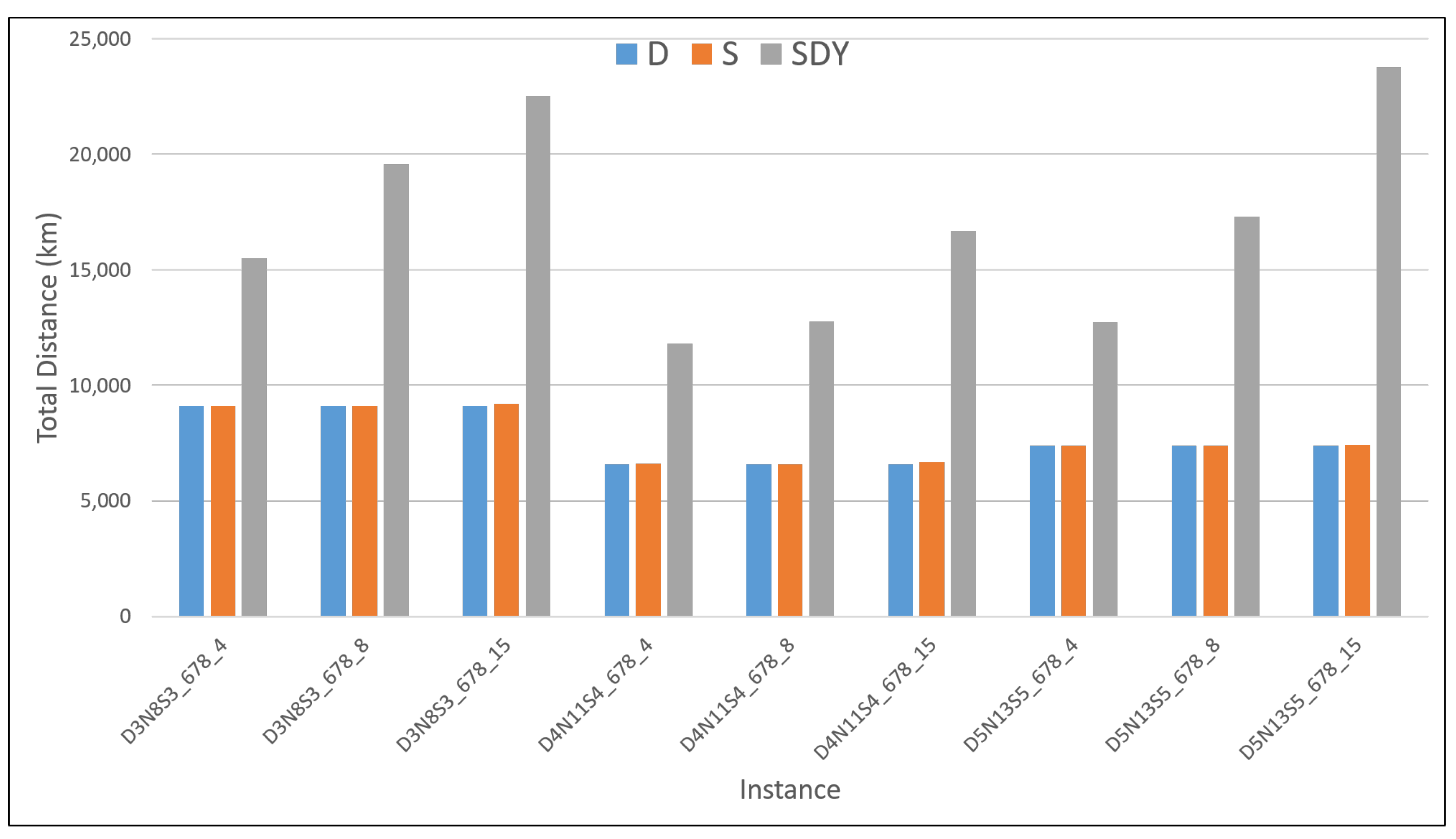
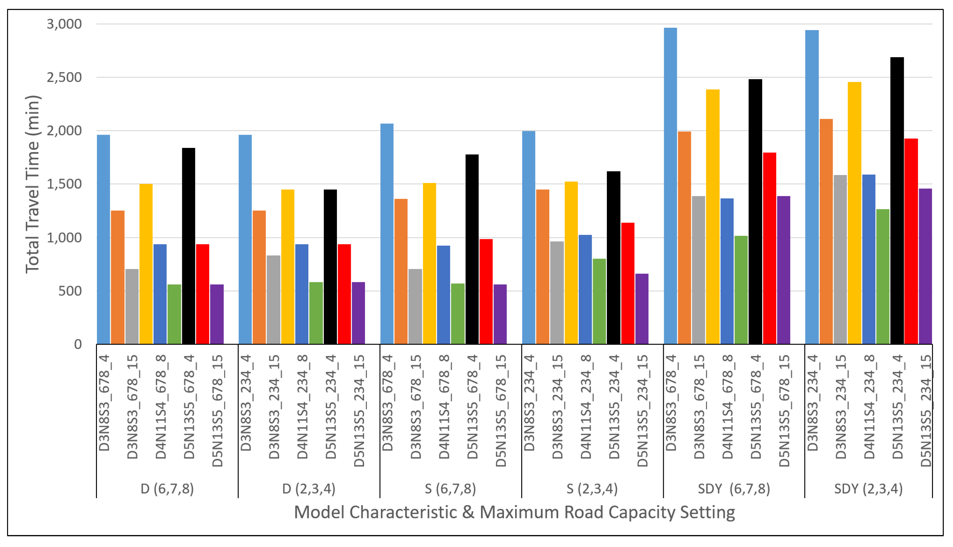
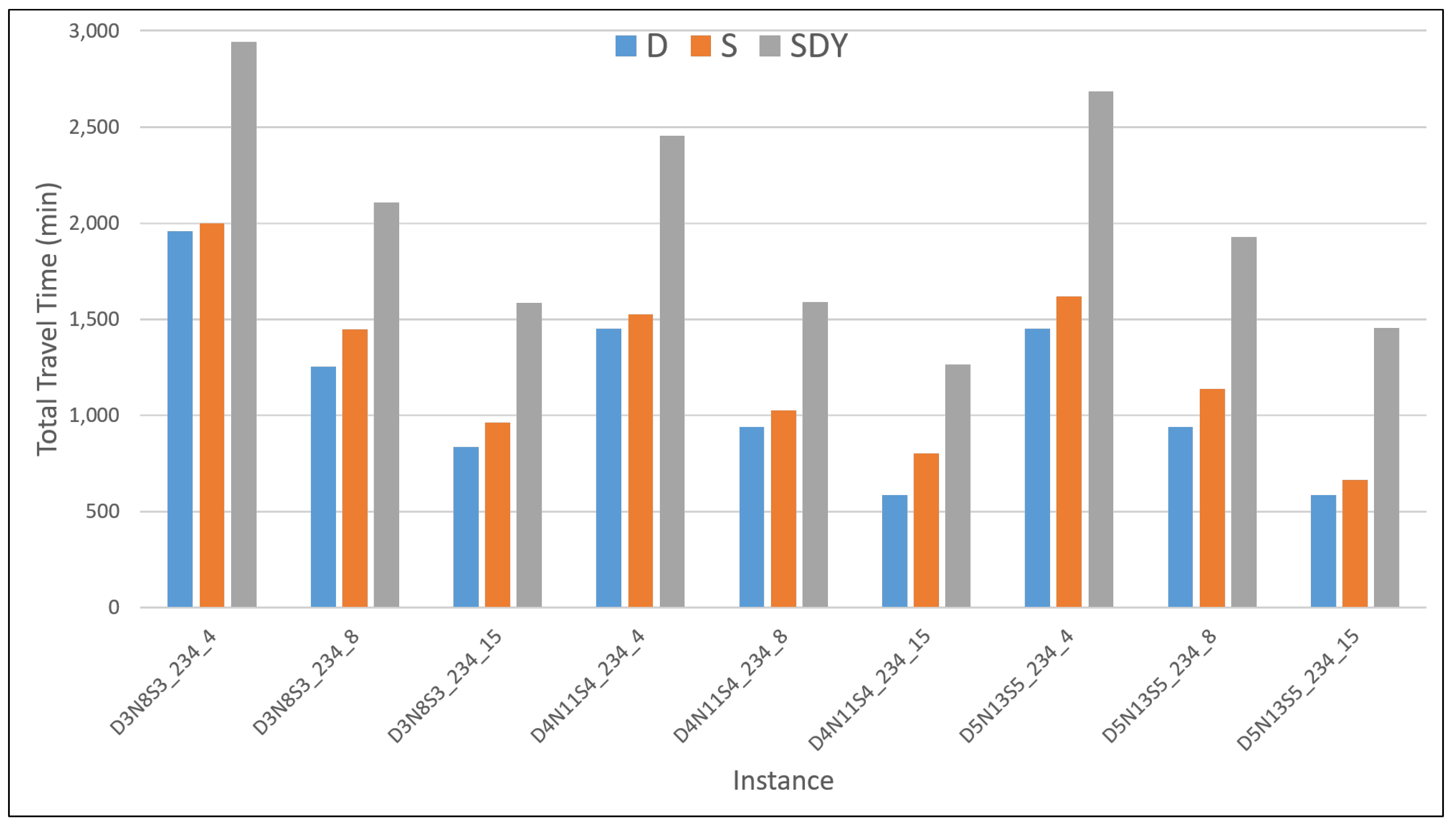
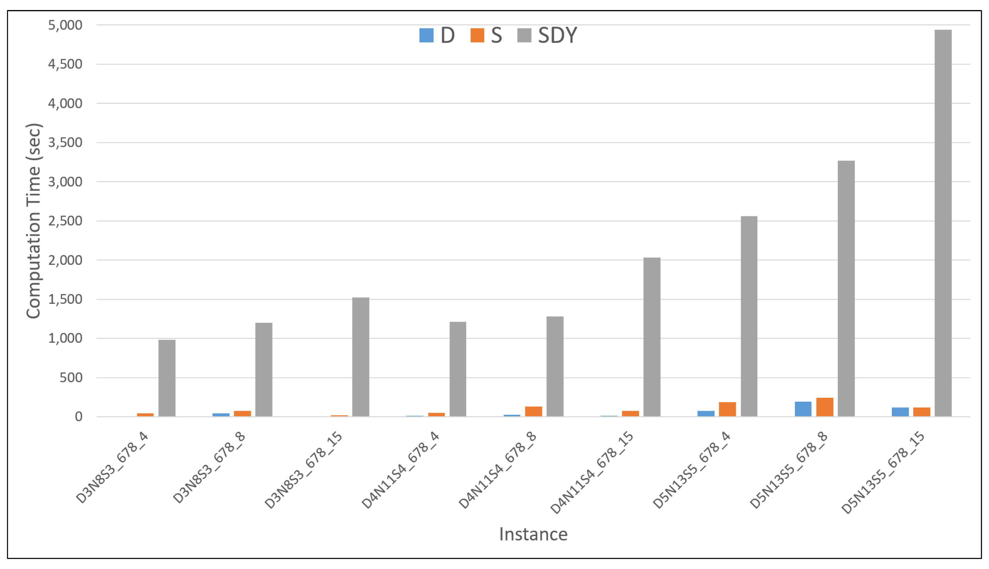
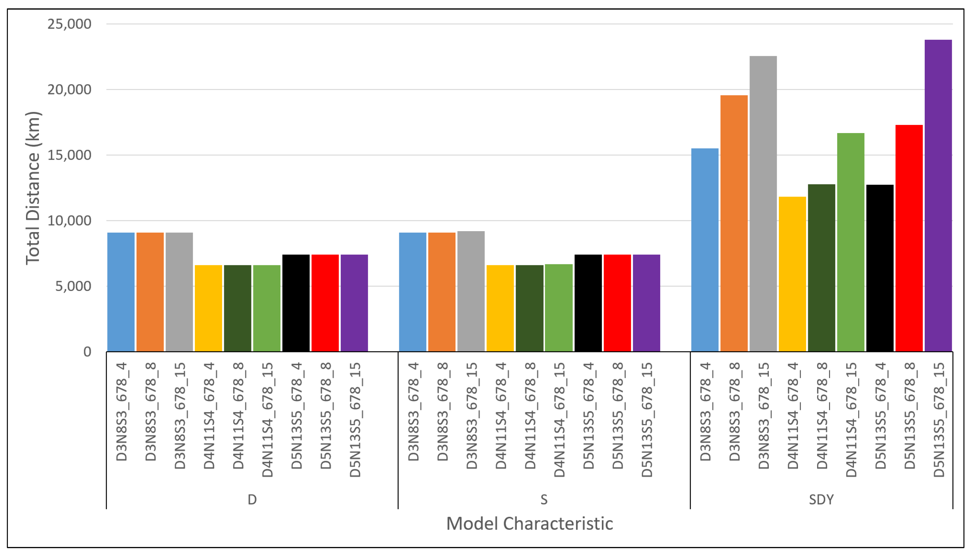
The results presented in the tables are translated into figures in Appendix A where observable trends could be seen. From the figures, it is obvious that addressing the online problem would result in covering much more total distance and thus would incur larger costs as compared to the results obtained through the offline computation of both the D-MDVRPRC and MDVRPSRC-2S as seen in Figure A5 and Figure A6 and especially Figure A14 and Figure A15.

The offline computation approach, however, is optimistic and unlikely to be realistic as both the D-MDVRPRC and MDVRPSRC-2S assume non dynamic changes with regards to road capacity. Therefore, the results obtained never consider some of the roads becoming increasingly less available over time for the vehicles. This is especially true for the roads in close proximity to the epicenter of the disaster. Addressing the online problem (using MDVRPSRC-2S1 and MDVRPSRC-2S2), however, took into account the dynamic reduction of road capacity over time due to damaged roads. Therefore, vehicle routes are developed constructively depending on the status of the road capacity at the time of decision point, $T_k$. Furthermore, the D-MDVRPRC and MDVRPSRC-2S models dispatch vehicles according to the total demands since they assume all the vehicles are able to travel safely back and forth from the depot. However, MDDVRPSRC takes into account the worst case scenario where the vehicle might be stranded at their last location due to no available road capacity to the neighboring location. Since the road capacity decreases over time, the vehicle might get stranded at any time throughout the mission. As a result, they could not make it back to the depot or resume delivery to shelters which are not fully served while en-route. This was observed a few times when running the smallest instance for the online computation where the roads to emergency shelters were limited and prone to damage. Thus, all vehicles are dispatched as long as total demands are not fully served. In a normal case scenario, the demand might be fully served when other vehicles with fresh capacity are dispatched and en-route, resulting in unnecessary trips. At this point, vehicles with non-delivered supplies have to return back to the depot from their assigned locations. This translates to additional distance or cost, total travel time as well as computation time.

Moreover, unlike D-MDVRPRC and MDVRPSRC-2S models, a realistic look at the problem assumes that, at the beginning, the vehicles are randomly distributed among the existing depots thus reflecting a more realistic situation during the disaster event. So, some vehicles might depart from depots that are situated at a location that is less ideal for an optimal delivery. The offline computation problem model has the luxury of choosing the departure depots for a respective vehicle in an optimal manner. All the aforementioned difference between offline and online models factored in towards a larger variance observed in the online model.

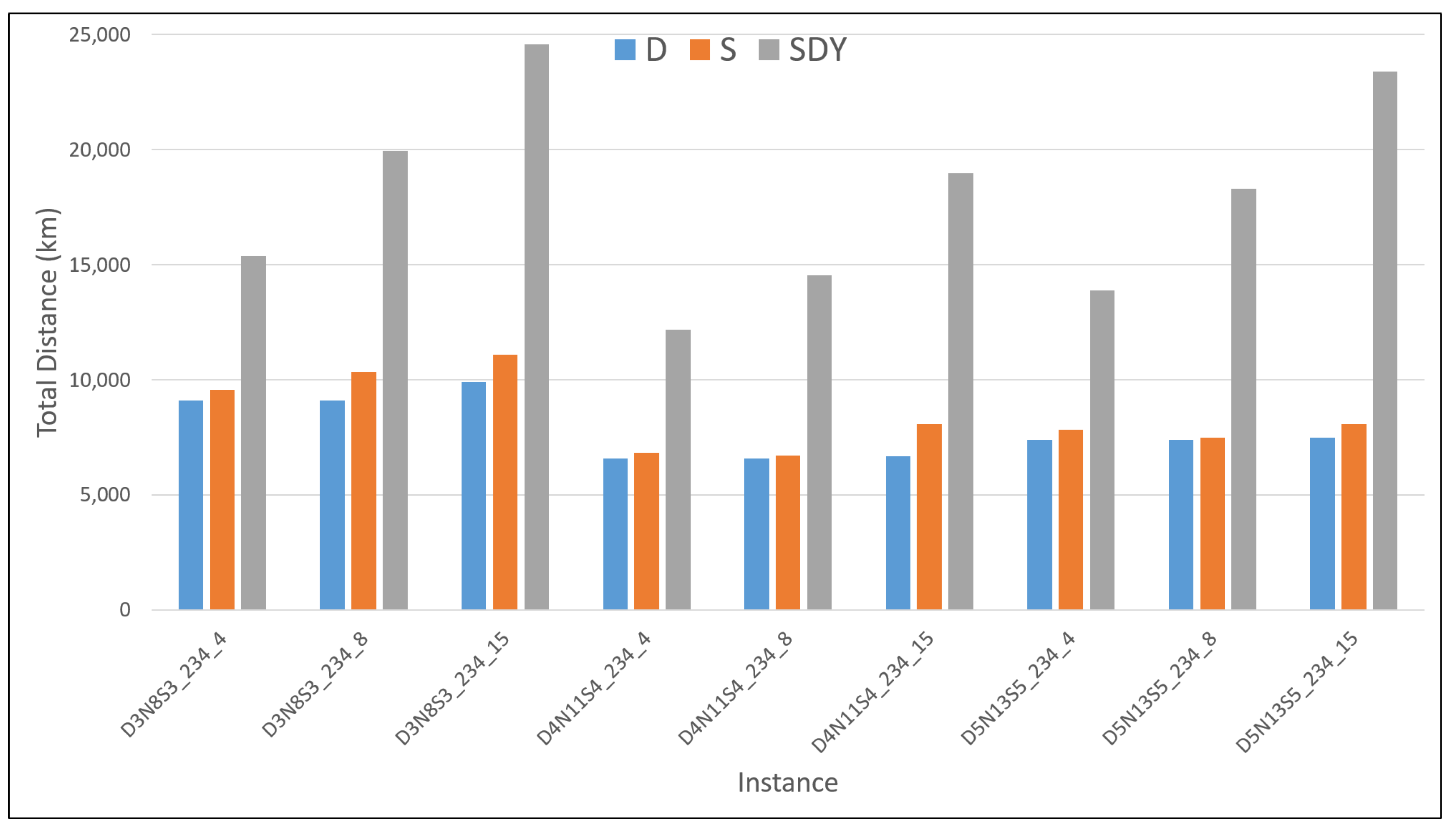
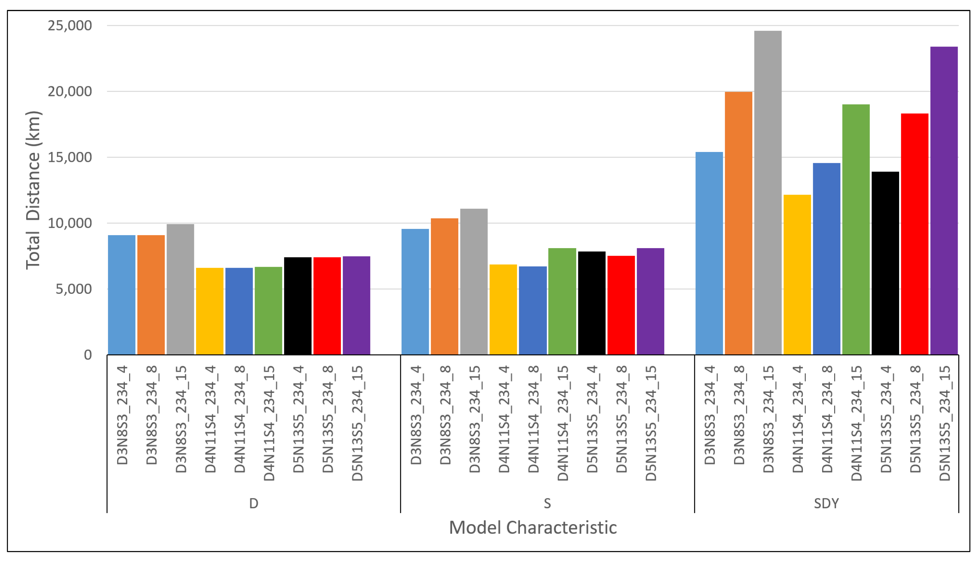
In Figure A5, Figure A6, Figure A7, Figure A8, Figure A9 and Figure A10, the total distance, total travel time and computation time are charted for every instance with respective maximum road capacity settings classified by their problem model: Deterministic (D), Stochastic programming (S) and the online MDDVRPSRC, which is both stochastic and dynamic (SDY). In Figure A5, especially, both offline computation models show close to no difference in terms of total distance travelled by the vehicle, even with the increase of vehicles from four, eight and 15 for all three instances. The SDY model, however, shows a clear increase of total distance travelled with the increased number of vehicles. Such observations could be explained by the difference in the mode of operations and assumptions taken between the offline and online modelling approach as explained earlier. The same reasoning would still apply for the slight increase of total distance for both S and D models seen in Figure A6, which addressed the instance with a tighter maximum road capacity setting. 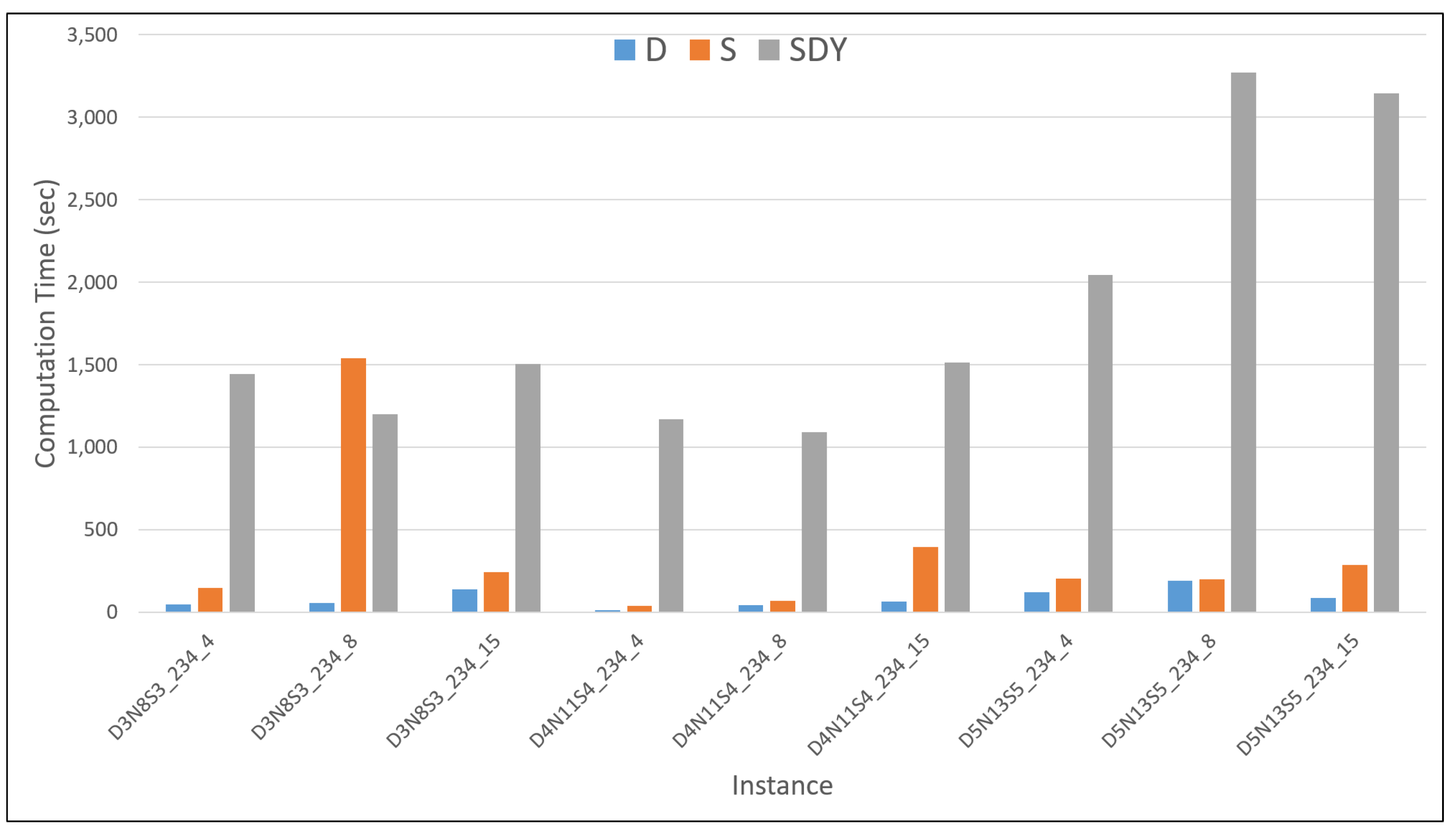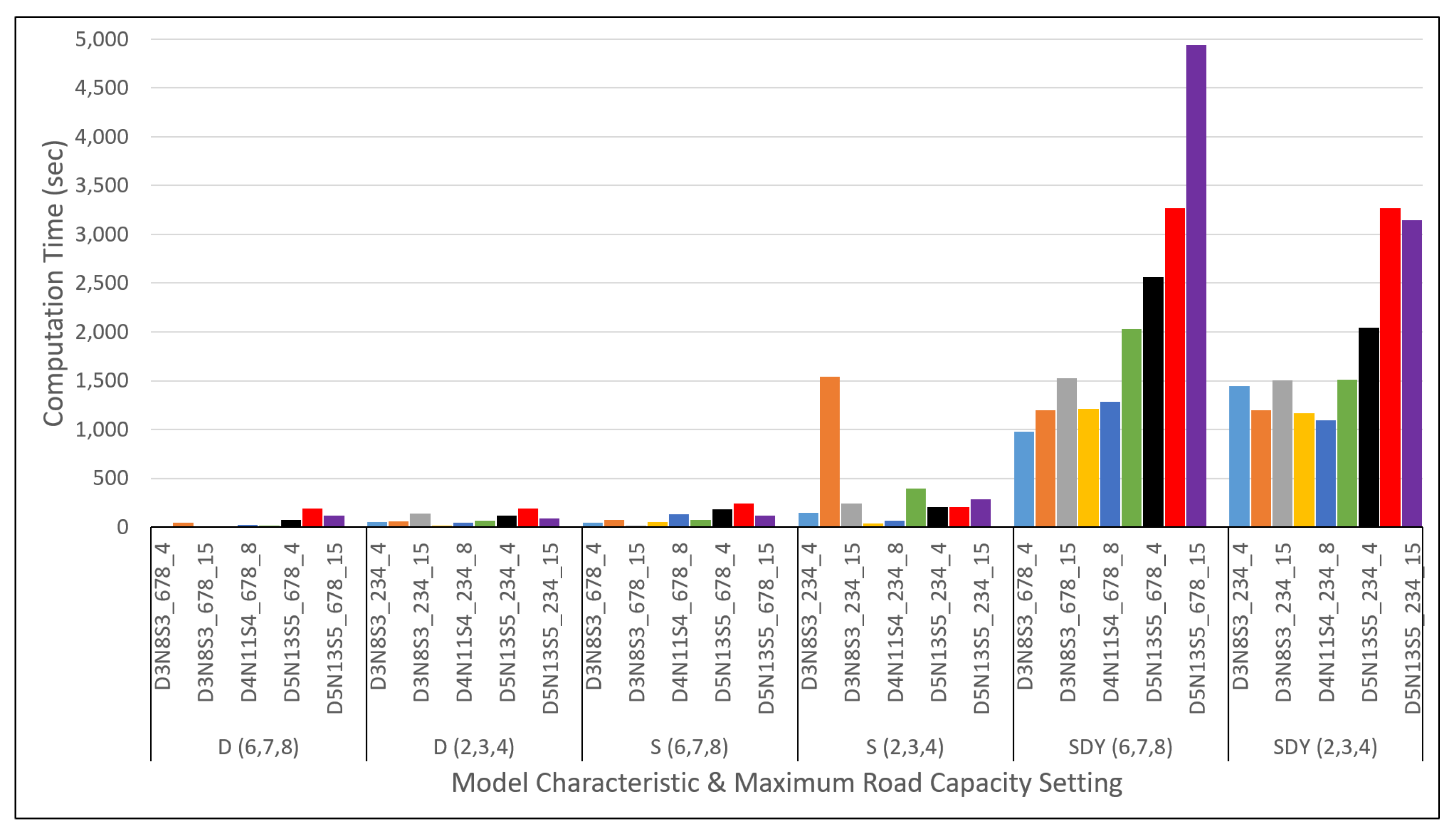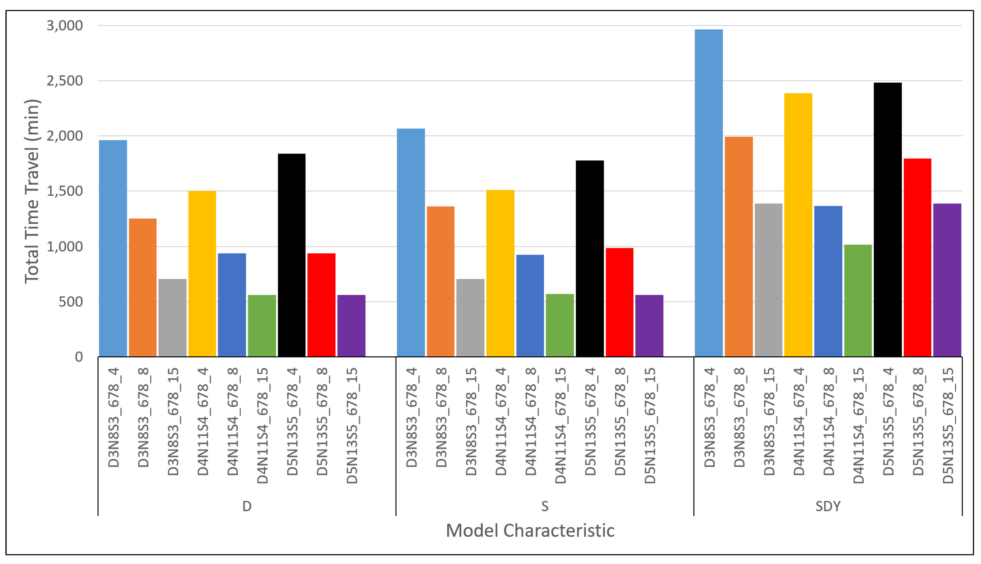In both Figure A7 and Figure A8, however, all three problem models solved for the routes show a decrease in time travel with the increase of vehicles. This result is to be expected as more vehicles may contribute to serving the total demands faster, proportional to the number of vehicles available. 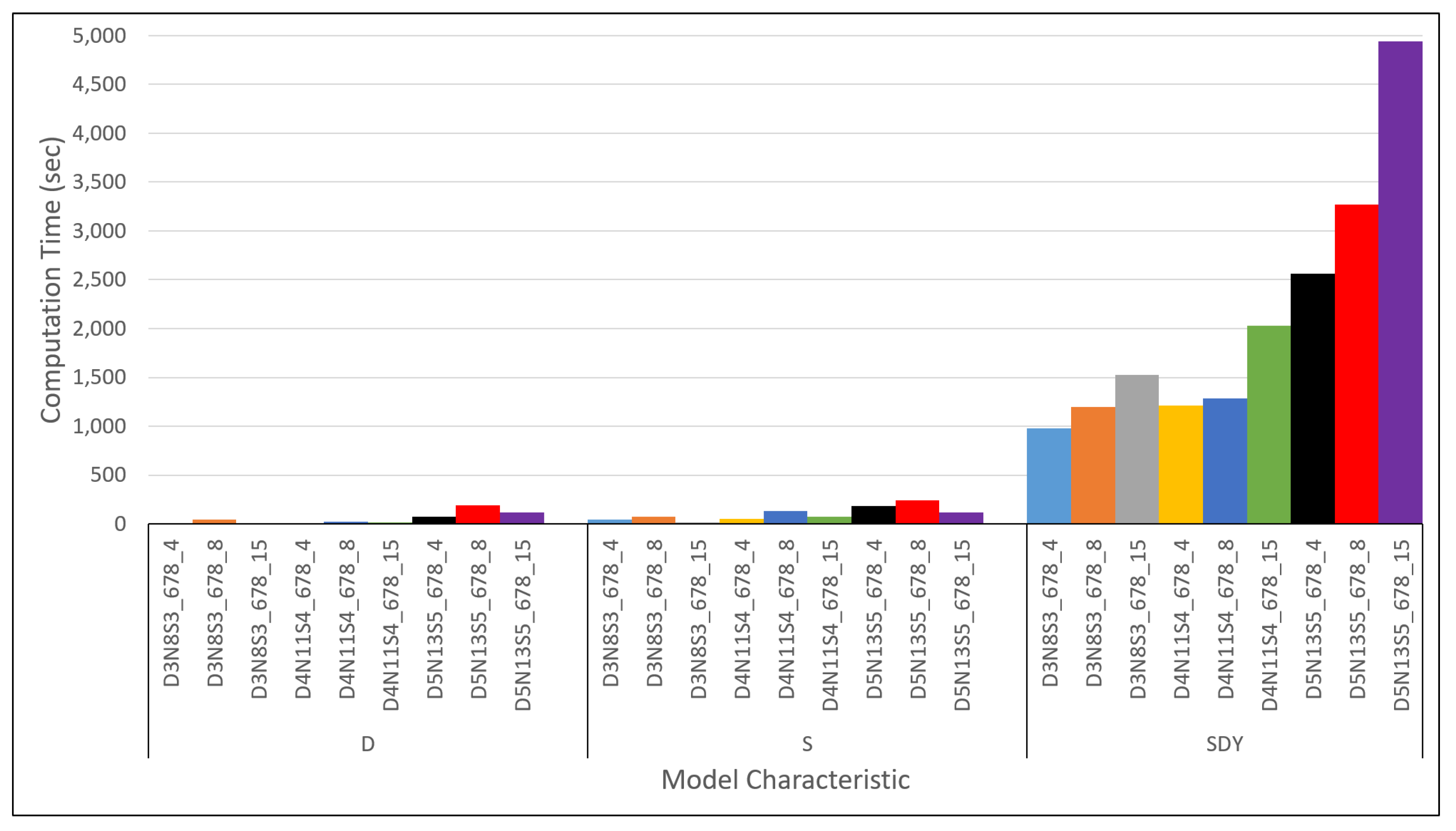Meanwhile, Figure A9 and Figure A10, as expected, show an overall increase of computation time for the D, S and SDY models in this order. An exception, however, is observed for a tighter maximum road capacity $(2,3,4)$. Here, the two-stage SILP model shows a huge jump in computation time for the smallest instance with 8 vehicles. This could be explained by a stochastic value of the road capacities based on the maximum capacity setting which might be sampled with small capacities where routing computation could be challenging.

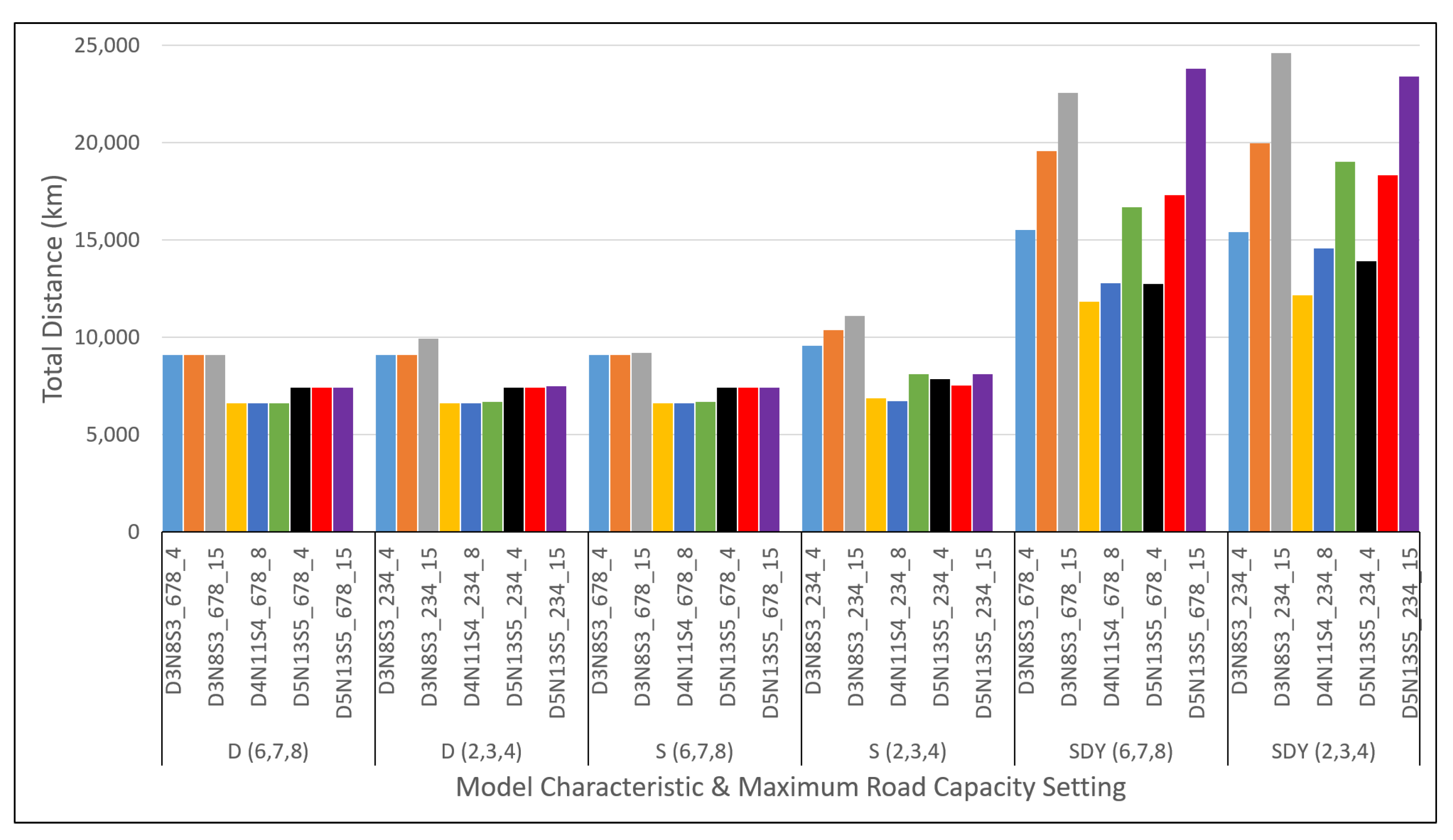
In Figure A11, Figure A12 and Figure A13, the assessment measurement values are compared side by side per instance, between the maximum road capacity settings $(6,7,8)$ and $(2,3,4)$. In general, the trend formed by the measured values could be said to be roughly similar where occasionally the setting $(2,3,4)$ would slightly increase the value of measurements. This is due to the consideration of the stochastic road capacity, which holds more influence for a tighter maximum road capacity setting. Roads with a maximum road capacity of two, for example, are more likely to be randomly sampled as zero during computation in comparison with roads with a maximum road capacity of six. Having one road perceived as unavailable for the offline computation would drastically deviate from the ideal optimal road configuration. This results in a slight difference in the value measured when compared to the results of the deterministic model. Here, it is also observed that an increase of vehicles for an instance with a tighter road capacity setting would also increase the total distance, especially for smaller instances. This is due to limited roads within the network (for smaller instances) that have a tighter capacity limit but need to accommodate a larger number of vehicles in order to reach the emergency shelters. For some vehicles, a direct or obvious route is not possible due to the capacity thus leading to a longer route detour resulting in an increase in total distance covered. Larger road networks, on the other hand, provided wider options for alternative routes even if a direct route is not possible.

Meanwhile, the counterparts of Figure A5, Figure A6, Figure A7, Figure A8, Figure A9 and Figure A10 (Figure A14, Figure A15, Figure A16, Figure A17, Figure A18 and Figure A19) are shown to observe the trends for all three instances, with increasing the amount of vehicles grouped by the model characteristics (D, S and SDY) for each maximum road capacity settings. Here, the general similarity of D and S model characteristics in terms of the results obtained for total distance, time travel as well as computation is even more apparent. Meanwhile, Figure A20, Figure A21 and Figure A22 are the counterparts of Figure A11, Figure A12 and Figure A13 where the trends obtained from Figure A14, Figure A15, Figure A16, Figure A17, Figure A18 and Figure A19 are put side by side based on their respective maximum road capacity settings. As discussed for the earlier figures, the MDVRPSRC-2S model tends to produce optimal assessment values similar to those of deterministic values when the stochastic sampling of random road capacity permits it. Otherwise, slight differences are observed, suggesting the limitation of ideal routes due to a tighter road capacity and thus road availability. It is also seen that the increase in the number of vehicles has close to no influence on decreasing the total distance travelled for the case of the two offline models. This is due to the flexibility of dispatching vehicles according to the total demand as well as the optimistic assumption that the vehicle dispatched will make it back to the depot.

6. Conclusions

This paper addressed the problem of Multi-Depot VRP with Stochastic Road Capacity during a post-disaster event for medical supplies’ delivery. Apart from multi-depot, split delivery is allowed to account for limited homogeneous vehicles when disaster strikes. The D-MDVRPRC model represents the deterministic version of the problem. The MDVRPSRC-2S model is based on the two-stage SILP in dealing with stochastic road capacity. Both of these models are validated by offline computations using CPLEX. Moreover, in this work, the reduced models from MDVRPSRC-2S: MDVRPSRC-2S1 and MDVRPSRC-2S2 are presented for iterative application during the rollout approach in ADP to solve MDDVRPSRC online. Through solving MDVRPSRC-2S1 or MDVRPSRC-2S2 for each vehicle at each decision point in the rollout, the base policy for rollout is thus constructed on the go.

All proposed models and the novel construction of the base policy in the rollout are validated through the results presented. From the results, the differences in the idealistic assumptions of the offline model and the more realistic online model are shown based on the solutions computed. Additionally, the dynamic consideration of deteriorating stochastic road capacity, which leads to difficulties in road navigation, is shown in the online computation of the problem. Based on the presented work, a few future research directions are noted. MDVRPSRC-2S addressed the problem by incorporating a recourse rule, which is to either to stay at the current position or to proceed with the computed route if the road capacity is available for the vehicle. This problem model could be extended with the option of navigating to other destinations instead of staying at the current position when the optimal path is not available. However, the model would be progressively complex as the extended version may need to be addressed by multi-stage stochastic programming instead of adapting to the multiple possible changes of routes at each route failure. Furthermore, the results obtained from the proposed rollout are based on a single vehicle rollout. More research can be carried out to study the practicality of such an approach (constructive matheuristic rollout) for the case of multiple-vehicle rollout in terms of reduced model complexity as well as additional computation time. The proposed solution approach, on the other hand, is shown to produce good results for a short rollout horizon and a minimal Monte Carlo simulation for this specific problem.

References

1. Zhao, B. April 2015 Nepal earthquake: Observations and reflections. Nat. Hazards 2016, 80, 1405–1410. [Google Scholar] [CrossRef]
2. Sharma, D.C. Nepal earthquake exposes gaps in disaster preparedness. Lancet 2015, 385, 1819–1820. [Google Scholar] [CrossRef]
3. Neupane, S.P. Immediate lessons from the Nepal earthquake. Lancet 2015, 385, 2041–2042. [Google Scholar] [CrossRef]
4. Menth, M.; Stamm, J.L.H. An agent-based modeling approach to improve coordination between humanitarian relief providers. In Proceedings of the Winter Simulation Conference (WSC), IEEE, Huntington Beach, CA, USA, 6–9 December 2015; pp. 3116–3117. [Google Scholar]
5. Radianti, J.; Hiltz, S.R.; Labaka, L. An overview of public concerns during the recovery period after a major earthquake: Nepal twitter analysis. In Proceedings of the System Sciences (HICSS), 2016 49th Hawaii International Conference on IEEE, Koloa, HI, USA, 5–8 January 2016; pp. 136–145. [Google Scholar]
6. Chiaro, G.; Kiyota, T.; Pokhrel, R.M.; Goda, K.; Katagiri, T.; Sharma, K. Reconnaissance report on geotechnical and structural damage caused by the 2015 Gorkha earthquake, Nepal. Soils Found. 2015, 55, 1030–1043. [Google Scholar] [CrossRef] [Green Version]
7. Archetti, C.; Savelsbergh, M.W.; Speranza, M.G. Worst-case analysis for split delivery vehicle routing problems. Transp. Sci. 2006, 40, 226–234. [Google Scholar] [CrossRef] [Green Version]
8. Ulmer, M.W. Approximate Dynamic Programming for Dynamic Vehicle Routing, 1st ed.; Operations Research/Computer Science Interfaces Series; Springer International Publishing: Berlin/Heidelberg, Germany, 2017; Volume 61. [Google Scholar]
9. Bellman, R.; Lee, E. History and development of dynamic programming. IEEE Control Syst. Mag. 1984, 4, 24–28. [Google Scholar] [CrossRef]
10. Bellman, R. The theory of dynamic programming. Bull. Am. Math. Soc. 1954, 60, 503–515. [Google Scholar] [CrossRef] [Green Version]
11. Anuar, W.K.; Lee, L.S.; Pickl, S.; Seow, H.V. Vehicle routing optimisation in humanitarian operations: A survey on modelling and optimisation approaches. Appl. Sci. 2021, 11, 667. [Google Scholar] [CrossRef]
12. Sepulveda, J.; Bull, J. A model-driven decision support system for aid in a natural disaster. In International Conference on Human Systems Engineering and Design: Future Trends and Applications; Springer: Berlin/Heidelberg, Germany, 2019; pp. 523–528. [Google Scholar]
13. Khorsi, M.; Chaharsooghi, S.K.; Bozorgi-Amiri, A.; Kashan, A.H. A multi-objective multi-period model for humanitarian relief logistics with split delivery and multiple uses of vehicles. J. Syst. Sci. Syst. Eng. 2020, 29, 360–378. [Google Scholar] [CrossRef]
14. Fragkos, M.E.; Zeimpekis, V.; Koutras, V.; Minis, I. Supply planning for shelters and emergency management crews. Oper. Res. 2020, 1–37. [Google Scholar] [CrossRef]
15. Vahdani, B.; Veysmoradi, D.; Shekari, N.; Mousavi, S.M. Multi-objective, multi-period location-routing model to distribute relief after earthquake by considering emergency roadway repair. Neural Comput. Appl. 2018, 30, 835–854. [Google Scholar] [CrossRef]
16. Ferrer, J.M.; Ortuño, M.T.; Tirado, G. A new ant colony-based methodology for disaster relief. Mathematics 2020, 8, 518. [Google Scholar] [CrossRef] [Green Version]
17. Yi, J.H.; Wang, J.; Wang, G.G. Using monarch butterfly optimization to solve the emergency vehicle routing problem with relief materials in sudden disasters. Open Geosci. 2019, 11, 391–413. [Google Scholar] [CrossRef] [Green Version]
18. Ferrer, J.M.; Martín-Campo, F.J.; Ortuño, M.T.; Pedraza-Martínez, A.J.; Tirado, G.; Vitoriano, B. Multi-criteria optimization for last mile distribution of disaster relief aid: Test cases and applications. Eur. J. Oper. Res. 2018, 269, 501–515. [Google Scholar] [CrossRef]
19. Wang, X.; Choi, T.M.; Liu, H.; Yue, X. A novel hybrid ant colony optimization algorithm for emergency transportation problems during post-disaster scenarios. IEEE Trans. Syst. Man Cybern. Syst. 2016, 48, 545–566. [Google Scholar] [CrossRef]
20. Nurprihatin, F.; Lestari, A. Waste collection vehicle routing problem model with multiple trips, time windows, split delivery, heterogeneous fleet and intermediate facility. Eng. J. 2020, 24, 55–64. [Google Scholar] [CrossRef]
21. Wang, L.; Kinable, J.; Van Woensel, T. The fuel replenishment problem: A split-delivery multi-compartment vehicle routing problem with multiple trips. Comput. Oper. Res. 2020, 118, 104904. [Google Scholar] [CrossRef]
22. Nugroho, S.; Nafisah, L.; Khannan, M.; Mastrisiswadi, H.; Ramdhani, M. Vehicle routing problem with heterogeneous fleet, split delivery, multiple product, multiple trip, and time windows: A case study in fuel distribution. In Proceedings of the IOP Conference Series: Materials Science and Engineering, Malang, East Java, Indonesia, 17–19 March 2020; Volume 847, p. 012066. [Google Scholar]
23. Hanum, F.; Hadi, M.; Aman, A.; Bakhtiar, T. Vehicle routing problems in rice-for-the-poor distribution. Decis. Sci. Lett. 2019, 8, 323–338. [Google Scholar] [CrossRef]
24. Yan, S.; Chu, J.C.; Hsiao, F.Y.; Huang, H.J. A planning model and solution algorithm for multi-trip split-delivery vehicle routing and scheduling problems with time windows. Comput. Ind. Eng. 2015, 87, 383–393. [Google Scholar] [CrossRef]
25. Artha, Y.E.B.; Santoso, S.; Liputra, D.T. Usulan Penentuan Rute Distribusi Dengan Multi Trip, Multi Product, dan Time Windows Menggunakan Algoritma Nearest Addition Heuristic. In Proceedings of the Seminar Nasional Teknik Industri Universitas Gadjah Mada, Yogyakarta, Indonesia, 5 October 2020; pp. 105–110. [Google Scholar]
26. Zhen, L.; Ma, C.; Wang, K.; Xiao, L.; Zhang, W. Multi-depot multi-trip vehicle routing problem with time windows and release dates. Transp. Res. Part Logist. Transp. Rev. 2020, 135, 101866. [Google Scholar] [CrossRef]
27. Khoukhi, S.; El Yaakoubi, O.; Bojji, C.; Bensouda, Y. A genetic algorithm for solving a multi-trip vehicle routing problem with time windows and simultaneous pick-up and delivery in a hospital complex. In Proceedings of the 3rd International Conference On Machine Learning and Soft Computing, Da Lat, Vietnam, 25–28 January 2019; pp. 76–80. [Google Scholar]
28. Jiang, Y.; Bian, B.; Liu, Y. Integrated multi-item packaging and vehicle routing with split delivery problem for fresh agri-product emergency supply at large-scale epidemic disease context. J. Traffic Transp. Eng. 2021, 8, 196–208. [Google Scholar]
29. Wang, D.; Zhu, J.; Wei, X.; Cheng, T.; Yin, Y.; Wang, Y. Integrated production and multiple trips vehicle routing with time windows and uncertain travel times. Comput. Oper. Res. 2019, 103, 1–12. [Google Scholar] [CrossRef]
30. Chen, R.M.; Guo, J.C. Optimal routing for split delivery vehicle routing problems. In Proceedings of the 2018 7th International Congress on Advanced Applied Informatics (IIAI-AAI), IEEE, Yonago, Japan, 8–13 July 2018; pp. 667–670. [Google Scholar]
31. Haghani, A.; Oh, S.C. Formulation and solution of a multi-commodity, multi-modal network flow model for disaster relief operations. Transp. Res. Part Policy Pract. 1996, 30, 231–250. [Google Scholar] [CrossRef]
32. Vogiatzis, C.; Yoshida, R.; Aviles-Spadoni, I.; Imamoto, S.; Pardalos, P.M. Livestock evacuation planning for natural and man-made emergencies. Int. J. Mass Emerg. Disasters 2013, 31, 25–37. [Google Scholar]
33. Shahabi, K.; Wilson, J.P. Scalable evacuation routing in a dynamic environment. Comput. Environ. Urban Syst. 2018, 67, 29–40. [Google Scholar] [CrossRef]
34. Tian, R.; Li, S.; Yang, G. Research on emergency vehicle routing planning based on short-term traffic flow prediction. Wirel. Pers. Commun. 2018, 102, 1993–2010. [Google Scholar] [CrossRef]
35. Zhan, S.L.; Chen, L.; Chen, P.K.; Ye, Y. A vehicle route planning method of two-phase large-scale crowd evacuation in typhoon relief activities. Math. Probl. Eng. 2019, 2019, 9539746. [Google Scholar] [CrossRef]
36. Shiripour, S.; Mahdavi-Amiri, N. Optimal distribution of the injured in a multi-type transportation network with damage-dependent travel times: Two metaheuristic approaches. Socio-Econ. Plan. Sci. 2019, 68, 100660. [Google Scholar] [CrossRef]
37. Yi, W.; Özdamar, L. A dynamic logistics coordination model for evacuation and support in disaster response activities. Eur. J. Oper. Res. 2007, 179, 1177–1193. [Google Scholar] [CrossRef]
38. Mohamed, R.E.; Kosba, E.; Mahar, K.; Mesbah, S. A framework for emergency-evacuation planning using GIS and DSS. In Information Fusion and Intelligent Geographic Information Systems (IF&IGIS’17); Springer: Berlin/Heidelberg, Germany, 2018; pp. 213–226. [Google Scholar]
39. Shiri, D.; Akbari, V.; Salman, F.S. Online routing and scheduling of search-and-rescue teams. OR Spectr. 2020, 42, 755–784. [Google Scholar] [CrossRef]
40. Ni, S.; Yu, J.; Zhong, Q. Routing design for emergency supplies based on multi-objective programming. In ICLEM 2014: International Conference of Logistics Engineering and Management; ASCE: Reston, VA, USA, 2014; pp. 463–469. [Google Scholar]
41. Zhou, X.; Tong, L.; Mahmoudi, M.; Zhuge, L.; Yao, Y.; Zhang, Y.; Shang, P.; Liu, J.; Shi, T. Open-source VRPLite package for vehicle routing with pickup and delivery: A path finding engine for scheduled transportation systems. Urban Rail Transit 2018, 4, 68–85. [Google Scholar] [CrossRef] [Green Version]
42. Lee, K.; Chae, J.; Song, B.; Choi, D. A model for sustainable courier services: Vehicle routing with exclusive lanes. Sustainability 2020, 12, 1077. [Google Scholar] [CrossRef] [Green Version]
43. Zhao, X.; Qian, W.w.; Huo, H. Multi-objective routing optimization for urban emergency rescue vehicles. In CICTP 2019: COTA International Conference of Transportation Professionals; ASCE: Reston, VA, USA, 2019; pp. 3855–3866. [Google Scholar]
44. Jiang, J.; Li, Q.; Wu, L.; Tu, W. Multi-objective emergency material vehicle dispatching and routing under dynamic constraints in an earthquake disaster environment. ISPRS Int. J. Geo Inf. 2017, 6, 142. [Google Scholar] [CrossRef] [Green Version]
45. Chen, D.; Yang, Z. Multiple depots vehicle routing problem in the context of total urban traffic equilibrium. J. Adv. Transp. 2017, 2017, 8524960. [Google Scholar] [CrossRef] [Green Version]
46. Dror, M.; Laporte, G.; Trudeau, P. Vehicle routing with stochastic demands: Properties and solution frameworks. Transp. Sci. 1989, 23, 166–176. [Google Scholar] [CrossRef]
47. Dror, M. Modeling vehicle routing with uncertain demands as a stochastic program: Properties of the corresponding solution. Eur. J. Oper. Res. 1993, 64, 432–441. [Google Scholar] [CrossRef]
48. Bertsekas, D.P.; Tsitsiklis, J.N.; Wu, C. Rollout algorithms for combinatorial optimization. J. Heuristics 1997, 3, 245–262. [Google Scholar] [CrossRef]
49. Secomandi, N. Comparing neuro-dynamic programming algorithms for the vehicle routing problem with stochastic demands. Comput. Oper. Res. 2000, 27, 1201–1225. [Google Scholar] [CrossRef]
50. Secomandi, N. Exact and Heuristic Dynamic Programming Algorithms for the Vehicle Routing Problem with Stochastic Demands. Ph.D. Thesis, University of Houston, Houston, TX, USA, 1998. [Google Scholar]
51. Secomandi, N. A rollout policy for the vehicle routing problem with stochastic demands. Oper. Res. 2001, 49, 796–802. [Google Scholar] [CrossRef]
52. Secomandi, N. Analysis of a rollout approach to sequencing problems with stochastic routing applications. J. Heuristics 2003, 9, 321–352. [Google Scholar] [CrossRef]
53. Novoa, C.M. Static and Dynamic Approaches for Solving the Vehicle Routing Problem with Stochastic Demands. Ph.D. Thesis, Lehigh University, Bethlehem, PA, USA, 2005. [Google Scholar]
54. Novoa, C.; Storer, R. An approximate dynamic programming approach for the vehicle routing problem with stochastic demands. Eur. J. Oper. Res. 2009, 196, 509–515. [Google Scholar] [CrossRef]
55. Fan, J.; Wang, X.; Ning, H. A multiple vehicles routing problem algorithm with stochastic demand. In Proceedings of the 2006 6th World Congress on Intelligent Control and Automation, IEEE, Dalian, China, 21–23 June 2006; Volume 1, pp. 1688–1692. [Google Scholar]
56. Goodson, J.C.; Ohlmann, J.W.; Thomas, B.W. Rollout policies for dynamic solutions to the multivehicle routing problem with stochastic demand and duration limits. Oper. Res. 2013, 61, 138–154. [Google Scholar] [CrossRef]
57. Powell, W.B. Approximate Dynamic Programming: Solving the Curses of Dimensionality; John Wiley & Sons: Hoboken, NJ, USA, 2007; Volume 703. [Google Scholar]
58. Goodson, J.C.; Thomas, B.W.; Ohlmann, J.W. Restocking-based rollout policies for the vehicle routing problem with stochastic demand and duration limits. Transp. Sci. 2016, 50, 591–607. [Google Scholar] [CrossRef]
59. Bertazzi, L.; Secomandi, N. Faster rollout search for the vehicle routing problem with stochastic demands and restocking. Eur. J. Oper. Res. 2018, 270, 487–497. [Google Scholar] [CrossRef]
60. Ulmer, M.W.; Mattfeld, D.C.; Hennig, M.; Goodson, J.C. A rollout algorithm for vehicle routing with stochastic customer requests. In Logistics Management; Springer: Berlin/Heidelberg, Germany, 2016; pp. 217–227. [Google Scholar]
61. Ulmer, M.W.; Goodson, J.C.; Mattfeld, D.C.; Hennig, M. Offline–online approximate dynamic programming for dynamic vehicle routing with stochastic requests. Transp. Sci. 2019, 53, 185–202. [Google Scholar] [CrossRef] [Green Version]
62. Bertazzi, L.; Bosco, A.; Guerriero, F.; Lagana, D. A stochastic inventory routing problem with stock-out. Transp. Res. Part Emerg. Technol. 2013, 27, 89–107. [Google Scholar] [CrossRef]
63. Moin, N.H.; Halim, H.Z.A. Solving inventory routing problem with stochastic demand. In AIP Conference Proceedings; AIP Publishing LLC: Melville, NY, USA, 2018; Volume 1974, p. 020104. [Google Scholar]
64. Zhao, Y.; Chen, X.; Jia, Q.S.; Guan, X.; Zhang, S.; Jiang, Y. Long-term scheduling for cascaded hydro energy systems with annual water consumption and release constraints. IEEE Trans. Autom. Sci. Eng. 2010, 7, 969–976. [Google Scholar] [CrossRef]
65. Bertazzi, L.; Bosco, A.; Laganà, D. Managing stochastic demand in an inventory routing problem with transportation procurement. Omega 2015, 56, 112–121. [Google Scholar] [CrossRef]
66. Dubois, F.; Renaud-Goud, P.; Stolf, P. Capacitated vehicle routing problem under deadlines. In Proceedings of the 2019 International Conference on Information and Communication Technologies for Disaster Management (ICT-DM), IEEE, Paris, France, 18–20 December 2019; pp. 1–8. [Google Scholar]
67. Goodson, J.C. Solution Methodologies for Vehicle Routing Problems with Stochastic Demand. Ph.D. Thesis, University of Iowa, Iowa City, IA, USA, 2010. [Google Scholar]
Figure 1. Damage Determination based on Interception on Edge due to Dispersion Radial Circle Representing Earthquake Tremor.
Mathematics 09 01572 g001
Figure 2. Proposed Matheuristic Rollout Concept for One Monte Carlo Episode.
Mathematics 09 01572 g002