Evaluation and Selection of the Quality Methods for Manufacturing Process Reliability Improvement—Intuitionistic Fuzzy Sets and Genetic Algorithm Approach

Abstract

The aim of this research is to propose a hybrid decision-making model for evaluation and selection of quality methods whose application leads to improved reliability of manufacturing in the process industry. Evaluation of failures and determination of their priorities are based on failure mode and effect analysis (FMEA), which is a widely used framework in practice combining with triangular intuitionistic fuzzy numbers (TIFNs). The all-existing uncertainties in the relative importance of the risk factors (RFs), their values, applicability of the quality methods, as well as implementation costs are described by pre-defined linguistic terms which are modeled by the TIFNs. The selection of quality methods is stated as the rubber knapsack problem which is decomposed into subproblems with a certain number of solution elements. The solution of this problem is found by using genetic algorithm (GA). The model is verified through the case study with the real-life data originating from a significant number of organizations from one region. It is shown that the proposed model is highly suitable as a decision-making tool for improving the manufacturing process reliability in small and medium enterprises (SMEs) of process industry.

1. Introduction

Nowadays, the problem of increasing reliability of manufacturing process, which represents the core of any industrial enterprise, affects the realization of business goals so that it is an interesting field of research for both researchers and practitioners. According to the results of the best practice, and literature sources [1], it can be said that failures have the greatest impact on the reliability of the manufacturing process. Although there is a significant number of production and organization concepts, such as world class manufacturing (WCM), just-in-time (JIT), the scope of this paper is set to the lean manufacturing and in compliance with that, failures leading to lean waste are identified. According to the lean concept [2], there are seven types of waste found in any process: transportation, inventory, motion, waiting, overprocessing, overproduction, and defect. Later, Liker [3] introduced waste related to underutilization of labor creativity, and it is denoted as Unused employee creativity. Reducing or eliminating the impact of identified failures can be performed by implementing various quality methods.

Quality methods are extremely important, because without reliable and complete information, it is practically impossible to undertake effective measures aimed at improving manufacturing processes [4,5].

There are many quality methods that are defined in the literature [6,7]. Application of these quality methods can lead to the simultaneous elimination or reduction of the impact of one or more identified failures of the manufacturing process. Respecting the limited resources (money, time, etc.), it can be concluded that it is almost impossible to implement a number of quality methods at the same time. In practice, the basic task of the reliability manager is how to choose a set of quality methods whose application of the considered problem can be effectively solved in the shortest possible time. Many authors suggest that the choice of quality methods should be based on the priority of failures [8,9,10,11]. Experiences of best practice show that decision makers (DMs), when choosing quality methods, respect many criteria besides the priority of failures. In this research, the authors suggest that in determining the set of quality methods, besides the mentioned, it is necessary to consider applicability of methods and implementation costs due to limited financial resources of small and medium enterprises in the manufacturing industry. Prioritization can be seen as a problem in itself. According to [12], the priority assessment under an uncertain environment is based on the failure mode and effect analysis (FMEA) which is combined with fuzzy sets theory [13], as in this research. In other words, evaluation of failures is performed by respecting to risk factors (RFs): severity, occurrence, and detection. According to suggestions of Liu [14], in this research, assumptions were introduced: (i) RFs have not equal the relative importance, and (ii) the relative importance of RFs and their values can be adequately described in linguistic terms, and (iii) the priority of failures is based on the rank of risk priority number (RPN) which is calculated as the product of these three RFs with respects to their weights.

Respecting the nature of human thinking, it can be said that DMs hardly give an accurate evaluation of uncertain data in practical decision problems. Hence, DMs express their assessments easier when using natural language words instead of the precise numbers. The development of theories of mathematics, such as the theory of intuitive fuzzy sets (IFSs) [15] allows vagueness to be represented fairly quantitatively. The advantages of using IFSs are: (1) transient stages during decision making can be rendered by intuitionistic indices, and (2) it is possible to foresee the best and worst results.

As it is known, in the manufacturing process management literature, it is almost impossible to find papers where the problem of choosing the quality methods set is considered as a combinatorial optimization problem. Since, in this research, the treated problem is stated as a rubber knapsack problem which represents the version of the classic 0–1 knapsack problem (0–1 KP) with the goal of finding, in a set of items of given values and weights, the subset of items with the highest total value, subject to a total weight constraint [16,17]. This can be marked as one of this paper’s novelties. Finding the optimal solution of the considered problem is based on using the genetic algorithm (GA) [18]. By using GAs, perform a search in complex, and large landscapes, and provide near-optimal solutions for objective function an optimization problem. In the literature, GA is a widely used metaheuristic method for solving difficult nondeterministic polynomial time (NP) problems from different domains [19,20,21], as in this research.

Motivation for this research comes from the fact that there are almost no literature sources that treat the selection of quality methods where uncertainties are given by exact ways.

The wider objective of this research may be interpreted as: (1) identification of failures in manufacturing process in SMEs of the process industry, (2) assessment identified failures based on FMEA, (3) modelling of the existing uncertainties are performed by using triangular intuitionistic fuzzy number (TIFN) [22,23], (4) the priority of failure is determined by applying the RPN with TIFNs with respects to RF weights, (6) selection of quality methods is stated as KP, and obtaining an adequate set of quality methods is based on the application of GA. The authors believe that the solution obtained in this way is significantly less burdened by the subjective attitudes of DMs, and therefore the effectiveness of solving the problem of reliability of the manufacturing process is significantly better.

The paper is organized in the following way: In Section 2, there is a literature review. Methodology is presented in Section 3. The proposed Algorithm is presented in Section 4. The case study is presented in Section 5. Conclusion and discussion are given in Section 6.

2. Literature Review

In the literature, there are no proposed procedures, rules, or recommendations on how to choose quality methods whose application improves the reliability of the manufacturing process. With the respect to the best industrial practice, it can be said that the choice of quality methods is always based on the knowledge and experience of reliability managers. In this way, the chosen set of quality methods is significantly burdened by the subjective attitudes of DMs. In order to increase the accuracy of the solution, in this research, the treated problem is stated as a discrete optimization problem and the solution is given by exact ways.

The classical KP can be defined as filling knapsack with a given set of objects with associated values, and space requirements associated with them although these problems have a simple structure, but they are known to be NP-hard. The KP has very important applications in the financial and industry domains, such as resource distribution, investment decision-making, items shipment, budget controlling, production planning [17], etc. There are many variants of KPs which are presented in the research literature.

In this research, the considered problem should be stated as KP which does not have a fixed value constraint. The knapsack constraint is not a specific value but a function of the number of solution elements. In the relevant literature, this version of KP is more complex than 0–1 KP and is relatively rarely investigated. The solution to this problem can be solved in different ways. In this paper, the solution to the considered problem is found by decomposing the given problem into subproblems with a certain number of solution elements. Each of the subproblems described above is a 2-dimensional KP. Each obtained solution can be further decomposed into several possible subversions due to the fact that many quality methods have the same applicability and/or implementation costs, so they are equivalent from the point of view of solution optimality.

Many researchers suggest applying GA for solving KPs [24,25]. Initially, GA generates randomly a population consisting of representative individuals (chromosomes) over which genetic operators of mutation, crossbreeding, and selection are successively applied. Fitness function is defined through the goal function of the considered problem. Based on the value of fitness function, a decision is made whether a representative individual remains in the population or not. In this way, a randomly selected population is transformed into a new population.

In classical KPs problems, all variables are described by precise numbers. In real life problems that exist in a changing environment, it is almost impossible to use precise measurement scales. Since, DMs better express their assessments of the relative importance and values of variables by using linguistic expressions. The development of theories of mathematics, such as the theory of fuzzy sets [13], has enabled these linguistic terms to be presented quantitatively in a sufficiently good way. In the literature, there are a large number of papers in which the relative importance of RFs and its values are modeled by: (i) type 1 fuzzy sets [26,27,28], (ii) the interval type 2 fuzzy numbers [10,29,30], and (iii) intuitionistic fuzzy sets [31,32,33]. The intuitionistic fuzzy set using two characteristic membership functions expressing the degree of membership and the degree of non-membership of elements of the universal set. It can cope with the presence of vagueness and hesitancy originating from imprecise [15]. It may be suggested that the natural language words can be adequately quantitatively described by using intuitionistic fuzzy sets.

Many authors suggest that the assessment of the relative importance of RFs should be set as a fuzzy group decision making problem. Aggregation DMs opinions into a single rating can be obtained by applying different operators, for instance: the intuitionistic fuzzy weighted average operator [34], intuitionistic fuzzy analytic hierarchy process [35,36], the utilized methods [37], fuzzy geometric mean [38], fuzzy averaging operator [39]. In this paper, all DMs originate from SMEs in which the same economic activity is realized, so to determine the aggregated value of the weight of risk RFs it is adequate to apply a fuzzy averaging operator as in [39].

3. Methodology

They base their assessments on knowledge and experience as well as data from records.

3.1. Basic Definitions of Intuitionistic Fuzzy Sets

Definition 1.

An intuitionistic fuzzy set A in the universe of discourse X is defined with the form [15]:

$$\tilde{A}=\left(x,{\mu }_{\tilde{A}}\left(x\right),{\vartheta }_{\tilde{A}}\left(x\right)|x\in X\right),$$

(1)

where:

The numbers${\mu }_{\tilde{A}}\left(x\right)\to \left[0,1\right]$and${\vartheta }_{\tilde{A}}\left(x\right)\to \left[0,1\right]$denote the membership degree and non-membership degree.

With the condition

$0\le {\mu }_{\tilde{A}}\left(x\right)+{\vartheta }_{\tilde{A}}\left(x\right)\le 1$, $\forall x\in X$

${\pi }_{\tilde{A}}\left(x\right)=1-{\mu }_{\tilde{A}}\left(x\right)-{\vartheta }_{\tilde{A}}\left(x\right)$

$0\le {\pi }_{\tilde{A}}\left(x\right)\le 1$, $\forall x\in X$

The value of${\pi }_{\tilde{A}}\left(x\right)$is called the degree of indeterminacy (or hesitation). The smaller${\pi }_{\tilde{A}}\left(x\right)$, more certain$\tilde{A}$.

Definition 2.

An IFS$\tilde{A}=\left(x, {\mu }_{\tilde{A}}\left(x\right),{\vartheta }_{\tilde{A}}\left(x\right)|x\in X\right)$of the real line is called an intuitonistic fuzzy number (IFN) whose membership function and non-membership function are defined as follows [40]:

$${\mu }_{\tilde{A}}\left(x\right)=\{\begin{array}{c}\begin{array}{ccc}\frac{x-a}{b-a}·{\mu }_{\tilde{A}}\left(x\right)& if& a\le x<b\\ {\mu }_{\tilde{A}}\left(x\right)& if& x=b\end{array}\\ \begin{array}{ccc}\frac{c-x}{c-b}·{\mu }_{\tilde{A}}\left(x\right)& if& b<x\le c\\ 0& & else\end{array}\end{array}$$

(2)

and

$${\vartheta }_{\tilde{A}}\left(x\right)=\{\begin{array}{c}\begin{array}{ccc}\frac{b-x+\left(x-a\right)·{\vartheta }_{\tilde{A}}\left(x\right)}{b-a}& if& a\le x<b\\ {\vartheta }_{\tilde{A}}\left(x\right)& if& x=b\end{array}\\ \begin{array}{ccc}\frac{x-b+\left(c-x\right)·{\vartheta }_{\tilde{A}}\left(x\right)}{c-b}& if& b<x\le c\\ 1& & else\end{array}\end{array}$$

(3)

where $a,b,c$ are real numbers, and $a\le b\le c$.

TIFN can be denoted as

$$\tilde{A}=\left(\left[a,b,c\right];{\mu }_{\tilde{A}}\left(x\right),{\vartheta }_{\tilde{A}}\left(x\right)\right),$$

(4)

Definition 3.

In compliance with the Definition 2, let$\tilde{A}=\left(\left[a_1,b_1,c_1\right];{\mu }_{\tilde{A}}\left(x\right),{\vartheta }_{\tilde{A}}\left(x\right)\right)$and$\tilde{B}=\left(\left[a_2,b_2,c_2\right];{\mu }_{\tilde{B}}\left(x\right),{\vartheta }_{\tilde{B}}\left(x\right)\right)$be two positive TIFNs. Additionally, λ is the real number. The operations of these TIFNs are given by [41]:

$$\tilde{A}+\tilde{B}=\left(\left[a_1+a_2,b_1+b_2,c_1+c_2\right];\min \left({\mu }_{\tilde{A}}\left(x\right),{\mu }_{\tilde{B}}\left(x\right)\right),\max \left({\vartheta }_{\tilde{A}}\left(x\right),{\vartheta }_{\tilde{B}}\left(x\right)\right)\right),$$

(5)

$$\tilde{A}-\tilde{B}=\left(\left[a_1-c_2,b_1-b,c_1-a_2\right];\min \left({\mu }_{\tilde{A}}\left(x\right),{\mu }_{\tilde{B}}\left(x\right)\right),\max \left({\vartheta }_{\tilde{A}}\left(x\right),{\vartheta }_{\tilde{B}}\left(x\right)\right)\right),$$

(6)

$$\tilde{A}·\tilde{B}=\left(\left[a_1·a_2,b_1·b_2,c_1·c_2\right];\min \left({\mu }_{\tilde{A}}\left(x\right),{\mu }_{\tilde{B}}\left(x\right)\right),\max \left({\vartheta }_{\tilde{A}}\left(x\right),{\vartheta }_{\tilde{B}}\left(x\right)\right)\right),$$

(7)

$$\mathsf{\lambda }·\tilde{A}=\left(\left[\mathsf{\lambda }·a_1,\mathsf{\lambda }·b_1,\mathsf{\lambda }·c_1\right];{\mu }_{\tilde{A}}\left(x\right),{\vartheta }_{\tilde{A}}\left(x\right)\right),$$

(8)

$${\tilde{A}}^{\mathsf{\lambda }}=\left(\left[a_1^{\mathsf{\lambda }},b_1^{\mathsf{\lambda }},c_1^{\mathsf{\lambda }}\right];{\mu }_{\tilde{A}}^{\mathsf{\lambda }}\left(x\right),\left(1-{\left(1-{\vartheta }_{\tilde{A}}\left(x\right)\right)}^{\mathsf{\lambda }}\right)\right),$$

(9)

$${\left(\tilde{A}\right)}^{-1}=\left(\left[\frac{1}{d_1},\frac{1}{c_1},\frac{1}{b_1},\frac{1}{a_1}\right];{\mu }_{\tilde{A}}\left(x\right),{\vartheta }_{\tilde{A}}\left(x\right)\right),$$

(10)

Definition 4.

A usual defuzzification method can be defined as mapping IFNs into scale value and taking the median [42], so that:

$$a=\frac{1}{12}·\left(a_1+4·b_1+c_1\right)·\left(1-{\vartheta }_{\tilde{A}}\left(x\right)+{\mu }_{\tilde{A}}\left(x\right)\right)$$

(11)

Definition 5.

Let$\tilde{A}=\left(\left[a_1,b_1,c_1\right];{\mu }_{\tilde{A}}\left(x\right),{\vartheta }_{\tilde{A}}\left(x\right)\right)$and$\tilde{B}=\left(\left[a_2,b_2,c_2\right];{\mu }_{\tilde{B}}\left(x\right),{\vartheta }_{\tilde{B}}\left(x\right)\right)$be two positive TIFNs. The Hamming distance [43] is:

$$d_H=\frac{1}{3}·\left(\left|a_1-a_2\right|+\left|b_1-b_2\right|+\left|c_1-c_2\right|\right)+\max \left(\left|{\mu }_{\tilde{A}}\left(x\right)-{\mu }_{\tilde{B}}\left(x\right)\right|,\left|\left({\vartheta }_{\tilde{A}}\left(x\right)-{\vartheta }_{\tilde{B}}\left(x\right)\right)\right|\right)$$

(12)

3.2. Definition of a Finite Set of Decision Makers

In this manuscript, the term DM means the FMEA team of each company. It is common for the FMEA team at the level of each company to be composed of: production manager, FMEA leader, and quality manager. It should be emphasized that they make the decision by consensus. DMs can be presented by the set e = {1, …, e, …E} The total number of considered DMs is marked with E, DM index e = 1, …, E.

3.3. Choice of Appropriate Linguistic Variables for Describing the Relative Importance of RFs

Defining a set of RFs against which failures are evaluated can be formally presented as a set $\left\{1,\dots ,k,\dots ,K\right\}$. Total number of RFs is denoted as K, and k, k = 1, ..., K is index of RF. In conventional FMEA [44] three RFs are defined: severity of consequence (k = 1), frequency of failure (k = 2), and possibility of detecting failure (k = 3), as in this research.

In compliance with the evidence from literature [10,14], the RFs may have different relative importance. The fuzzy rating of the relative importance of RFs are based on the pre-defined linguistic expressions and their corresponding TIFNs are presented in the Table 1.

Table 1. The relative importance of RFs.

	TIFNs
low importance (L)	$\left(\left[1,1,3.5\right];0.8,0.1\right)$
medium importance (M)	$\left(\left[1,3.5,5\right];0.6,0.3\right)$
high importance (H)	$\left(\left[2.5,5,5\right];0.7,0.2\right)$

The domains of these TIFNs are defined into real line into interval [1–5]. The value 1 indicates the lowest and the value 5 the highest relative importance of the considered RFs. The overlap of TIFNs describing the relative importance of RFs is large. This indicates a lack of knowledge of DMs about the importance of the considered criteria in SMEs of the manufacturing sector.

3.4. Choice of Appropriate Linguistic Variables for Describing the RF Values, Aplicability of Quality Methods, and Implementation Costs of Quality Methods

In the production process, numerous failures can occur, which can be formally represented by the set of indices $\left\{1, \dots , i,\dots ,I\right\}$, where I presents the total number of failures, and the index of each failure is denoted as i, I = 1, …, I. In this research, failures that are identified at the level of each observed SME are considered.

Analysis and reduction of the identified failures can be performed by applying numerous quality methods that can be formally represented by the set of indices $\left\{1, \dots , m,\dots ,M\right\}$. The total number of quality methods is denoted as M, and m, m = 1, ..., M is index of quality method. In this research, quality methods are selected according to [6].

The evaluation of the value of RFs, ${\tilde{v}}_{ik}$ is performed by DM at the level of each SME. Applicability of quality method m for failure analysis i, ${\tilde{v}}_{mi}$, I = 1, ..., I, are assessed by quality manager at the level of each considered SME and presented in Table 2.

Table 2. The RF values and degree of belief that quality methods are applicable.

	TIFNs
very low value (VLV)	$\left(\left[1, 1, 2.5\right];0.65,0.3\right)$
low value (LV)	$\left(\left[2, 3.5, 5\right];0.7,0.25\right)$
medium value (MV)	$\left(\left[3.5, 5, 6.5\right];0.5,0.45\right)$
high value (HV)	$\left(\left[6, 7.5, 9\right];0.75,0.2\right)$
very high value (VHV)	$\left(\left[7.5, 9, 9\right];0.8,0.15\right)$

The domains of these TIFNs are defined in the common measurement scale [1–9]. The value 1 indicates the lowest and the value 9 indicates the highest values of RFs.

Implementation costs of considered quality methods, ${\tilde{c}}_m$ were evaluated by the quality manager and presented in Table 3.

Table 3. Implementation costs.

	DESCRIPTION	TIFNs
Extremely low cost (C1)	Implementing quality methods requires almost no cost	$\left(\left[0, 0.1, 0.25\right];0.7,0.25\right)$
Very low value (C2)	The implementation of the quality method does not require equipment	$\left(\left[0.1, 0.3, 0.6\right];0.65,0.3\right)$
Medium value (C3)	Implementing the method requires standard equipment	([0.3,0.55,0.7];0.55,0.4)
High value (C4)	Implementation of quality methods requires the use of computer equipment	$\left(\left[0.5, 0.75, 0.9\right];0.6,0.3\right)$
Very high value (C5)	Implementation of quality methods requires expensive specialized equipment	$\left(\left[0.7, 0.95, 1\right];0.65,0.3\right)$

The domains of these TIFNs are defined in the common measurement scale [0, 1]. The value 0 indicates the lowest and the value 1 indicates the highest values of implementation costs.

4. The Proposed Algorithm

Step 1. The relative importance of RF k, k = 1, ..., K is assessed by each DM e, e = 1, .., E:

$${\tilde{W}}_k^e$$

(13)

Step 2. The aggregated relative importance of RF k, ${\tilde{W}}_k$, k = 1, ..., K, is given by using fuzzy averaging operator:

$${\tilde{W}}_k=\frac{1}{E}·{\tilde{W}}_k^e$$

(14)

Step 3. The representative scalar of TIFN, ${\tilde{W}}_k$, $W_k$, k = 1, ..., K is given by using the defuzzification procedure [42].

Step 4. Construct the weights vector of RFs, ${\left[{\omega }_k\right]}_{1\times K}$. The element of weights vector of RFs,${\omega }_k$ given by using the linear normalization procedure, so that:

$${\omega }_k=\frac{W_k}{{{\displaystyle \sum }}_{k=1,\dots ,K}{W}_k}$$

(15)

Step 5. The value of each RF, k = 1, ..., K for each failure i, I = 1, ..., I is assessed by DM and could be presented by TIFN, ${\tilde{v}}_{ik}$.

Step 6. Determine the priority index for each failure i, I = 1, ..., I by using fuzzy geometric mean:

$${\widetilde{RPN}}_i={\displaystyle \prod }_{k=1,\dots ,K}{\left({\tilde{v}}_{ik}\right)}^{{\omega }_k}$$

(16)

Step 7. Degree of beliefs that quality methods are applicable to the analysis of identified failure, ${\tilde{v}}_{mi}$ and costs of implementation of quality methods, ${\tilde{c}}_m$ are assessed by DM.

Step 8. Determine the applicability of the quality method, ${\tilde{z}}_{mi}$, to eliminate failure i, m = 1, ..., M; I = 1, ..., I:

$${\tilde{z}}_{mi}={\tilde{v}}_{mi}·{\widetilde{RPN}}_i$$

(17)

Step 9. The normalized value of applicability of the quality method m at the level of failure i, m = 1, ..., M; I = 1, ..., I, is:

$${\tilde{r}}_{mi}=\frac{{\tilde{z}}_{mi}}{{\tilde{z}}^{*}}$$

(18)

where, ${\tilde{z}}^{*}$ is the maximum applicability of the method, so that:

$${\tilde{z}}^{*}=VHV{\displaystyle \prod }_{k=1,\dots ,K}{\left(VHV\right)}^{{\omega }_k}$$

(19)

Step 10. The total applicability of the method m, m = 1, ..., M is obtained according to the expression:

$${\tilde{r}}_m=\underset{i=1,\dots ,I}{\max }\left({\tilde{r}}_{mi}\right)$$

(20)

Ranking of uncertain values, ${\tilde{r}}_{mi}$ is performed according to crisp values $r_{mi}$, so that:

$$r_m=\underset{i=1,\dots ,I}{\max }defuzz\left({\tilde{r}}_{mi}\right)$$

(21)

Step 11. Let us set the KP problem:

The fitness function:

$$\underset{j=1,\dots ,J}{\max }{\displaystyle \sum }_{}d{\left({\tilde{r}}_m,{\tilde{c}}_m\right)}_j,j\in \left\{1,\dots ,m,\dots ,M\right\}$$

(22)

where, $d\left({\tilde{r}}_m,{\tilde{c}}_m\right)$ is calculated as the Hamming distance between two TIFNs [43].

The objective to:

$$\frac{1}{J-1}·{\displaystyle \sum }_{j=1,\dots ,J}{\left(d\left({\tilde{c}}_m,\tilde{c}\right)\right)}^2\le \frac{1}{M-1}·{\displaystyle \sum }_{m=1,\dots ,M}{\left(d\left({\tilde{c}}_m,\tilde{c}\right)\right)}^2{}^{}$$

(23)

where:

$$\tilde{c}=\frac{1}{M}·{\displaystyle \sum }_{m=1,\dots ,M}{\tilde{c}}_m$$

And

$$d{\left({\tilde{r}}_m,{\tilde{c}}_m\right)}_j=\{\begin{array}{cc}1& ifobjectjisselected\\ 0& otherwise\end{array}$$

(24)

Step 12. The near optimal solution of the treated KP problem is found by using GA. The encoding schemes are differentiated according to the problem domain. The well-known encoding schemes are binary, octal, hexadecimal, value-based, and tree. Binary encoding is the used encoding scheme in this paper. Each chromosome is represented using a binary string. In binary encoding, every chromosome is 0 or 1. In knapsack problem, binary encoding is used in GA to show the presence of items, 1 for the presence of an item and 0 for the absence of an item.

The initial parameter setting with a population of 100 individuals was gradually reduced to 30 without loss in solution quality, also a further increase in the number of interactions over 1000 was not significant.

The parameters of the applied GA are: generational GA, roulette wheel parent selection, elitism 0.05%, number of individuals in the population 30, selection 0.95, mutation 0.02, and number of iterations 1000. Furthermore, a part of the code of the implemented GA is given, which provides the condition that the chromosome has a precisely determined number of units. In this way, the generation of correct units is ensured without the need for subsequent rejection of defective ones. The following part of the code is given below:

• public string Generate(int NumberOfAllMeasures, int NumberOfMeasures)
• {
• string ret = new String(‘0’, NumberOfAllMeasures);
• int[] measuresRB = new int[NumberOfAllMeasures];
• double[] measuresRand = new double[b NumberOfAllMeasures];
• for (int i = 1; i <= NumberOfAllMeasures; i++)
• {
• measuresRB[i-1] = i-1;
• measuresRand[i-1] = random.NextDouble();
• }
• Array.Sort(measuresRand, measuresRB);
• char[] ch = ret.ToCharArray();
• for (int i = 1; i <= NumberOfMeasures; i++)
• {
• ch[measuresRB[i-1]] = ‘1’;
• }
• return new string(ch);

5. Case Study

In this research, the research is realized in 24 manufacturing SMEs located in Bosnia and Herzegovina (B&H). Respecting the official data, it can be said that: (i) account of considered SMEs for more than 15% of total gross domestic product (GDP), (ii) about 20% of total employment in B&H, and (iii) almost 90% of exports, such as they have a significant impact on economic growth in B&H. Experiences of good practice show that one of the most important problems of an operational management team is to maintain the reliability of the manufacturing process over a long period of time. In this way, the defined business goals of the company can be realized to a high degree. Improving the reliability of the manufacturing process is realized through the accurate identification of potential failures and through the selection of adequate quality methods by which the identified failures are reduced and/or eliminated.

As is known in the literature, there are no procedures or recommendations on how to identify failures in manufacturing processes or how to choose quality methods, which leads to increased reliability of the manufacturing process. Experiences of best practice in the process industry show that failure identification is always based on evidence data and experience and knowledge of decision makers, as in this research. The set of quality methods that can potentially be applied is defined according to the recommendations from the relevant literature.

Assessment of the relative importance of RFs, their values, applicability of treated quality methods, as well as the costs of implementation were obtained using the interview method. Questionnaires were sent to the FMEA team asking them to express all estimates using the given pre-defied linguistic expressions. They also returned the completed questionnaires by e-mail.

The Illustration of the Proposed Model

Fuzzy assessment of the relative importance of RFs is performed by DM at the level of each SME (Step 1 of the proposed Algorithm). This is presented in Table 4.

Table 4. Fuzzy rating of the relative importance of RFs.

	E = 1	E = 2	E = 3	E = 4	E = 5	E = 6	E = 7	E = 8	E = 9	E = 10	E = 11	E = 12	E = 13	E = 14	E = 15	E = 16	E = 17	E = 18	E = 19	E = 20	E = 21	E = 22	E = 23	E = 24
K = 1	H	H	M	H	H	M	H	H	H	M	H	H	H	M	H	H	H	M	H	H	H	H	H	M
K = 2	H	M	M	M	M	M	M	H	H	L	M	M	M	M	M	M	M	L	H	M	H	H	M	M
K = 3	L	H	H	M	H	H	L	M	M	L	L	L	L	L	M	M	L	M	M	L	M	M	L	H

The proposed aggregation and defuzzification procedures (Step 2 to Step 3 of the proposed Algorithm) is illustrated for example (k = 1):

$${\tilde{W}}_1=\frac{1}{24}·\left(18·H+6·M\right)=\frac{1}{24}·\left(\left[51,111,120\right];0.6,0.3\right)=\left(\left[2.13,4.63,5\right];0.6,0.3\right)$$

The precise number of TIF ${\tilde{W}}_1$, $W_1$ is:

$$W_1=\frac{1}{12}·\left(2.13+4·4.63+5\right)·\left(1-0.3+0.6\right)=2.776$$

Similarity, the relative importance of the rest RFs are given:

$$\begin{gathered} {\tilde{W}}_2=\left(\left[1.375,3.666,4.875\right];0.6,0.3\right)\mathrm{and}{W}_2=2.266 \\ {\tilde{W}}_3=\left(\left[1.312,2.771,4.375\right];0.6,0.3\right)\mathrm{and}{W}_3=1.817 \end{gathered}$$

The weights vector (Step 4 of the proposed Algorithm) is:

$$\begin{gathered} {\omega }_k=\frac{W_k}{{{\displaystyle \sum }}_{k=1,\dots ,K}{W}_k} \\ \left[\begin{array}{ccc}0.40,& 0.33,& 0.26\end{array}\right] \end{gathered}$$

The assessment values of RFs for SME (e = 1) are given in a Table 5 (Step 5 of the proposed Algorithm):

Table 5. Fuzzy rating of the relative importance of RFs.

Lean Waste	Failures	S	O	D	Lean Waste	Failures	S	O	D
Overprocessing	Inadequate level of automation (I = 1)	HV	HV	VLV	Overproduction	Inadequate use of automation (I = 23)	VLV	VLV	HV
	Inadequate processing modes (I = 2)	MV	LV	MV		Poor assessment of market demands (I = 24)	MV	LV	MV
	Worker error (I = 3)	MV	MV	MV		Poor application of just in case logic (I = 25)	HV	MV	MV
	Product design requires too many processing steps (I = 4)	LV	VLV	VLV		Low knowledge and skills of employees (I = 26)	LV	MV	VLV
	Too many processing processes, too many iterations (I = 5)	MV	LV	VLV	Motion	Poor workplace ergonomics (I = 27)	VLV	HV	VLV
	Customer needs are not clear (I = 6)	VHV	LV	HV		Large distance between operations (I = 28)	MV	MV	VLV
Inventory	Imbalance of material flow (I = 7)	LV	LV	VLV		Frequent hand movements (I = 29)	HV	MV	LV
	The unreliability of suppliers (I = 8)	LV	VLV	VLV		Multiple taking the same piece (I = 30)	MV	HV	LV
	Excessive supply of raw materials (I = 9)	VHV	VLV	VLV		Employees have to move to get information (I = 31)	MV	MV	MV
	Poor communication (I = 10)	LV	LV	LV		Manual work to compensate for some shortcomings in the production process (I = 32)	MV	MV	MV
	Protection of the company from risk and unexpected event (I = 11)	MV	VLV	LV		Inexperience of the operator (I = 33)	HV	MV	LV
Transportation	Not understanding the process flow (I = 12)	VLV	VLV	LV	Waiting	Waiting for material between operations (I = 34)	LV	LV	VLV
	Inadequate layout of technological equipment (I = 13)	MV	LV	VLV		Interruption of the machine or system (I = 35)	MV	MV	VLV
	Large storage space (I = 14)	LV	VLV	VLV		Lack of work (I = 36)	HV	MV	VLV
	Communication failure (I = 15)	VLV	MV	LV		Waiting for the information needed to continue the process (I = 37)	MV	VLV	MV
	Using old layouts (I = 16)	VLV	VLV	VLV		Imbalance with subsequent processes (I = 38)	MV	MV	MV
Defect	Insufficient knowledge and skills of workers (I = 17)	MV	MV	MV		Long preparatory-final time (I = 39)	MV	VLV	MV
	Inaccuracies in the documentation (I = 18)	VHV	LV	LV	Unused employee creativity	Narrowly defined jobs (I = 40)	MV	LV	VLV
	Insufficient process control (I = 19)	HV	MV	MV		Not involving workers in creating new ideas (I = 41)	LV	MV	MV
	Design-construction omissions (I = 20)	MV	VLV	LV		Employees do not work in the appropriate position (I = 42)	MV	LV	LV
	Inadequate state of technical and technological equipment (I = 21)	MV	VLV	MV		Not involving all employees and their knowledge and skills in business and production processes (I = 43)	MV	MV	MV
Overproduction	Imbalance of production lines (I = 22)	MV	LV	LV		Workers’ absenteeism (I = 44)	MV	MV	MV

The proposed procedure (Step 6 of the proposed Algorithm) is illustrated for the failure (I = 1):

$$\begin{gathered} {\widetilde{RPN}}_1={\left(\left[6,7.5,9\right];0.75,0.2\right)}^{0.40}·{\left(\left[6,7.5,9\right];0.75,0.2\right)}^{0.33}·{\left(\left[1,1,2.5\right];0.65,0.3\right)}^{0.26} \\ {\widetilde{RPN}}_1=\left(\left[2.07,2.26,2.43\right];0.89,0.09\right)·\left(\left[1.81,1.95,2.07\right];0.91,0.07\right)·\left(\left[1,1,1.27\right];0.89,0.09\right) \\ =\left(\left[3.73,4.40,6.41\right];0.89,0.09\right) \end{gathered}$$

RPN values for all other failures were calculated in a similar way and shown in Appendix A.

According to the proposed procedure (Step 7 of the proposed Algorithm), the degree of beliefs is calculated.

Applicability of methods with respects to priority failures as well as calculation of normalized values (Step 8 to Step 9 of the proposed Algorithm) is illustrated in the following example:

$$\begin{gathered} {\tilde{z}}_{61}={\tilde{v}}_{61}·{\widetilde{RPN}}_1=\left(\left[6,7.5,9\right];0.75,0.2\right)·\left(\left[3.73,4.40,6.41\right];0.89,0.09\right) \\ =\left(\left[27.41,47.08,66.70\right];0.75,0.20\right) \end{gathered}$$

Let the maximum applicability of the method be given by using the expression (4.7):

$$\begin{gathered} {\tilde{z}}^{*}=\left(\left[7.5,9,9\right];0.8,0.15\right){\displaystyle \prod }_{k=1,\dots ,3}{\left(\left[7.5,9,9\right];0.8,0.15\right)}^{0.4}·{\left(\left[7.5,9,9\right];0.8,0.15\right)}^{0.33} \\ ·{\left(\left[7.5,9,9\right];0.8,0.15\right)}^{0.26}=\left(\left[55.12,79.24,79.24\right];0.8,0.15\right) \end{gathered}$$

So that, the normalized assessment of the applicability of the method (m = 6) at the level of failure (i = 1) is:

$${\tilde{r}}_{61}=\frac{\left(\left[27.41,47.08,66.70\right];0.75,0.20\right)}{\left(\left[55.12,79.24,79.24\right];0.8,0.15\right)}=\left(\left[0.35,0.59,1.21\right];0.75,0.20\right)$$

To apply the proposed procedure (Step 10 of the proposed Algorithm) it is necessary to determine representative scalars, so that:

$$r_{61}=\frac{1}{12}·\left(0.35+4·0.59+1.21\right)·\left(1-0.2+0.75\right)=0.506$$

Ranking of uncertain values, ${\tilde{r}}_{61}$ is performed according to crisp values $r_{61}$, so that:

$$\begin{gathered} r_6=\underset{i=1,\dots ,I}{\max }defuzz\left(\begin{array}{c}0.178;0.169;0.413;0.076;0.120;0.506;0.105;0.078;0.230;0.137;0.274;0.066;0.258;0.080;0.101;0.043;0.413;\\ 0.418;0.486;0.243;0.268;0.156;0.080;0.204;0.487;0.117;0.089;0.133;0.208;0.191;0.191;0.204;0.227;0.289;\\ 0.340;0.149;0.199;0.129;0.120;0.167;0.156;0.191;0.191\\ \end{array}\right) \\ =0.506 \end{gathered}$$

Therefore:

$${\tilde{r}}_{61}=\left(\left[0.35,0.59,1.21\right];0.55,0.4\right)$$

In the same way, each quality method m, m = 1 ,.., M is accompanied by the normalized total applicability shown in Table 6. The same table shows the other input data.

Table 6. Input data.

	${\tilde{\mathit{r}}}_{\mathit{m}}$	${\tilde{\mathit{c}}}_{\mathit{m}}$	$\mathit{d} \left({\tilde{\mathit{r}}}_{\mathit{m}}, {\tilde{\mathit{c}}}_{\mathit{m}}\right)$	${\left(\mathit{d}\left({\tilde{\mathit{c}}}_{\mathit{m}},\tilde{\mathit{c}}\right)\right)}^2$
M = 1	$\left(\left[0.34,0.59,1.21\right];0.5,0.45\right)$	C3	0.2467	0.0215
M = 2	$\left(\left[0.34,0.59,1.21\right];0.5,0.45\right)$	C3	0.2467	0.0215
M = 3	$\left(\left[0.09,0.22,0.62\right];0.5,0.45\right)$	C2	0.1867	0.0187
M = 4	$\left(\left[0.27,0.47,1.12\right];0.5,0.45\right)$	C2	0.4367	0.0187
M = 5	$\left(\left[0.27,0.47,1.12\right];0.5,0.45\right)$	C2	0.4367	0.0187
M = 6	$\left(\left[0.34,0.59,1.21\right];0.5,0.45\right)$	C2	0.5300	0.0187
M = 7	$\left(\left[0.43,0.71,1.28\right];0.5,0.45\right)$	C2	0.6233	0.0187
M = 8	$\left(\left[0.01,0.02,0.16\right];0.5,0.45\right)$	C2	0.4200	0.0187
M = 9	$\left(\left[0.01,0.02,0.16\right];0.5,0.45\right)$	C2	0.4200	0.0187
M = 10	$\left(\left[0.09,0.18,0.58\right];0.5,0.45\right)$	C2	0.2000	0.0187
M = 11	$\left(\left[0.06,0.10,0.41\right];0.5,0.45\right)$	C2	0.2933	0.0187
M = 12	$\left(\left[0.17,0.34,0.86\right];0.5,0.45\right)$	C2	0.2733	0.0187
M = 13	$\left(\left[0.22,0.42,1.03\right];0.5,0.45\right)$	C4	0.3967	0.1995
M = 14	$\left(\left[0.06,0.10,0.41\right];0.5,0.45\right)$	C2	0.2933	0.0187
M = 15	$\left(\left[0.10,0.16,0.57\right];0.5,0.45\right)$	C2	0.1867	0.0187
M = 16	$\left(\left[0.06,0.10,0.41\right];0.5,0.45\right)$	C2	0.2933	0.0187
M = 17	$\left(\left[0.10,0.16,0.57\right];0.5,0.45\right)$	C2	0.1867	0.0187
M = 18	$\left(\left[0.10,0.16,0.57\right];0.5,0.45\right)$	C1	0.3600	0.1627
M = 19	$\left(\left[0.43,0.71,1.28\right];0.5,0.45\right)$	C2	0.6233	0.0187
M = 20	$\left(\left[0.34,0.59,1.21\right];0.5,0.45\right)$	C2	0.5300	0.0187
M = 21	$\left(\left[0.43,0.71,1.28\right];0.5,0.45\right)$	C2	0.6233	0.0187
M = 21	$\left(\left[0.43,\mathrm{0.711.28}\right];0.5,0.45\right)$	C2	0.233	0.0187
M = 22	$\left(\left[0.34,0.59,1.21\right];0.5,0.45\right)$	C2	0.5300	0.0187
M = 23	$\left(\left[0.34,0.59,1.21\right];0.5,0.45\right)$	C5	0.4867	0.3762
M = 24	$\left(\left[0.12,0.19,0.57\right];0.5,0.45\right)$	C2	0.2033	0.0187
M = 25	$\left(\left[0.01,0.02,0.16\right];0.5,0.45\right)$	C2	0.4200	0.0187
M = 26	$\left(\left[0.34,0.59,1.21\right];0.5,0.45\right)$	C4	0.3600	0.1995
M = 27	$\left(\left[0.34,0.59,1.21\right];0.5,0.45\right)$	C2	0.5300	0.0187
M = 28	$\left(\left[0.20,0.39,0.92\right];0.5,0.45\right)$	C4	0.3767	0.1995
M = 29	$\left(\left[0.43,0.71,1.28\right];0.5,0.45\right)$	C2	0.6233	0.0187
M = 30	$\left(\left[0.01,0.02,0.16\right];0.5,0.45\right)$	C2	0.4200	0.0187
M = 31	$\left(\left[0.01,0.02,0.16\right];0.5,0.45\right)$	C2	0.4200	0.0187
M = 32	$\left(\left[0.01,0.02,0.16\right];0.5,0.45\right)$	C2	0.4200	0.0187
M = 33	$\left(\left[0.06,0.10,0.41\right];0.5,0.45\right)$	C3	0.3767	0.0215
M = 34	$\left(\left[0.01,0.02,0.16\right];0.5,0.45\right)$	C2	0.4200	0.0187
M = 35	$\left(\left[0.43,0.71,1.28\right];0.5,0.45\right)$	C2	0.6233	0.0187
M = 36	$\left(\left[0.34,0.59,1.21\right];0.5,0.45\right)$	C2	0.5300	0.0187
M = 37	$\left(\left[0.01,0.02,0.16\right];0.5,0.45\right)$	C2	0.4200	0.0187
M = 38	$\left(\left[0.34,0.59,1.21\right];0.5,0.45\right)$	C2	0.5300	0.0187
M = 39	$\left(\left[0.34,0.59,1.21\right];0.5,0.45\right)$	C2	0.5300	0.0187
M = 40	$\left(\left[0.34,0.59,1.21\right];0.5,0.45\right)$	C2	0.5300	0.0187
M = 41	$\left(\left[0.34,0.59,1.21\right];0.5,0.45\right)$	C2	0.5300	0.0187
M = 42	$\left(\left[0.34,0.59,1.21\right];0.5,0.45\right)$	C2	0.5300	0.0187
M = 43	$\left(\left[0.43,0.71,1.28\right];0.5,0.45\right)$	C2	0.6233	0.0187
M = 44	$\left(\left[0.34,0.59,1.21\right];0.5,0.45\right)$	C2	0.5300	0.0187
M = 45	$\left(\left[0.35,0.61,1.19\right];0.5,0.45\right)$	C2	0.5333	0.0187
M = 46	$\left(\left[0.43,0.71,1.28\right];0.5,0.45\right)$	C2	0.6233	0.0187
M = 47	$\left(\left[0.34,0.59,1.21\right];0.5,0.45\right)$	C2	0.5300	0.0187
M = 48	$\left(\left[0.34,0.59,1.21\right];0.5,0.45\right)$	C2	0.5300	0.0187
M = 49	$\left(\left[0.34,0.59,1.21\right];0.5,0.45\right)$	C1	0.8467	0.1627

Determine the mean value of implementation costs:

$$\tilde{c}=\frac{1}{49}·{\displaystyle \sum }_{m=1,\dots ,49}{\tilde{c}}_m=\left(\left[0.14,0.35,0.62\right];0.55,0.40\right)$$

And the variance of implementation costs:

$$\frac{1}{49-1}·{{\displaystyle \sum }}_{m=1,\dots ,49}d{\left(d\left({\tilde{c}}_m,\tilde{c}\right)\right)}^2=\frac{1}{48}·2.1117=0.044$$

Assumed that the reliability manager should select 10 quality methods. This assumption was introduced based on best practice experience. Under this assumption, the KP problem (Step 11 of the proposed Algorithm) is:

The objective function

$$\underset{j=1,\dots ,10}{\max }d{\left({\tilde{r}}_m,{\tilde{c}}_m\right)}_j,j\in \left\{1,\dots ,m,\dots ,M\right\}$$

The objective to:

$$\frac{1}{9}·{\displaystyle \sum }_{j=1,\mathrm{..10}}{\left(d\left({\tilde{c}}_m,\tilde{c}\right)\right)}^2\le 0.04$$

GA (Step 12 of the proposed Algorithm) was applied to find a near-optimal solution. The stop criterion is defined to have a number of iterations equal to 1000.

It has been shown that about 300 iterations are achieved near the optimal solution (see Figure 1).

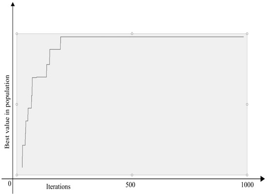
Figure 1. Value of fitness function by iterations.

For the near-optimal solution, the solution obtained in the last iteration was adopted:

By applying GA, the quality methods that the reliability manager in the considered company should implement in order to eliminate failures, or increase the reliability of the manufacturing process is:

solution 1: $\left\{m=7, m=19, m=21, m=29, m=35, m=38, m=43, m=45, m=46, m=49\right\}$

solution 2: $\left\{m=7, m=19, m=21, m=22, m=29, m=35, m=43, m=45, m=46, m=49\right\}$

It is worth to mention that the treated problem could be solved by the branch and bound algorithm [45] but it has a significant limitation since it is applicable to the lower size problems. In the presented case study, the output of the GA and branch and bound algorithm does not indicate output results deviation. As the number of quality methods in practice is increasing, the application of GA seems to be more adequate due to the nonpalatability of the branch and bound algorithm.

Based on the results of the survey, it can be concluded that most quality tools can be successfully applied to the analysis and identification of failures, which will ultimately lead to the elimination of failures, and thus lean waste. The obtained results show 10 methods that need to be applied in order to finally eliminate failures and increase the reliability of the manufacturing process. These methods can be implemented simultaneously. The period of implementation and education of employees for the implementation of these methods is not long. Another important fact is that the implementation of the above methods is not faced with the challenge of reorganization. The organizational culture of different SMEs will affect the effectiveness of the application of methods, so the effectiveness of the application should be observed at the level of each individual enterprise. In SMEs that have implemented the total quality management (TQM) and quality system according to the ISO 9001 standard, most of these tools are already in use and do not require additional investment and additional costs for the application of these methods.

This new problem-solving approach sets the standard for those who are just applying the problem-solving approach, as well as for those who are interested in continuously improving existing problem-solving methodologies.

6. Conclusions

As continuous changes that occur both in the company and in the environment impact the overall business performance, improving the reliability of the manufacturing process is one of the most important problems of operational management. This might be very significant since a reliable manufacturing process further positively impacts the stability of other business processes and enables competitive advantages in the long run. Experiences of best practice show that improving the reliability of the manufacturing process depends on the knowledge and experience of the FMEA team to identify failures as well as the knowledge of quality managers to choose quality methods by which identified failures can be eliminated or reduced leading to improved reliability of the manufacturing process.

In this research, identification of failures that can occur in manufacturing processes of considered SMES, is performed by FMEAs and based on their knowledge and experience as well as on best practice experience. The identified failures are assessed with respects to the RFs which are defined according to the FMEA framework. The set of possible quality methods are defined according to literature sources [6].

It is assumed that it is closer to the human way of thinking that the existing uncertainties into the relative importance of RFs, their values, application possibilities, as well as application costs of quality methods can be described better by using pre-defined linguistic expressions. These linguistic terms are modeled by the TIFNs. It can be said that the use of TIFNs does not require complex mathematical calculations and at the same time, linguistic terms are quantitatively described in a sufficiently good way.

Respecting to the results of the best practice, it can be said that the choice of quality methods depends on several variables. In this research, it is assumed that quality managers simultaneously consider the overall applicability of the method and implementation costs. The overall applicability of quality methods at the level of each failure is calculated as the product of the estimated degree of belief that the application of the quality method can lead to the reduction or elimination of failures and fuzzy weighted RPN with TIFNs associated with each failure. Determination weights of failures is sated as a fuzzy group decision making problem. In the literature, there are almost no papers in which procedures have been developed in which the choice of the quality method is made in an exact way. In this manuscript, the treated problem is stated as KP whose: (i) fitness function is defined as the distance between total applicability and implementation costs, and (ii) constraint is defined as a function of the number of solution elements. Near optimal solution with respect to fitness function and given constraints, simultaneously, may be efficiently achieved by small consumption of computation resources through the application of the GA.

The main advantage in theoretical terms of the presented model that combines FMEA, intuitive fuzzy sets [15], KP, and GA are: (i) that DMs can express their estimates using natural language words which in a good enough way can be quantitatively described by TIFNs, (ii) selection of a set of quality methods whose application can effectively increase the reliability of the manufacturing process while minimizing the consumption of financial resources. In this way, prioritizing quality methods is not significantly burdened by subjective attitudes of the quality manager, which would be one of the main advantages of this way of defining the improvement strategy.

The proposed model can be quickly and easily adjusted due to changes in the number of failures, number of quality methods, as well as their values.

The general limitations of the model are the need for a well-structured list of failures that can be realized in the manufacturing process in the production of SMEs.

Future research could include the extension of the proposed model in terms of: (1) increasing the number of variables on which fitness function depends and (3) applying other metaheuristic methods and comparing the obtained results.

References

- Karaulova, T.; Kostina, M.; Sahno, J. Framework of Reliability Estimation for Manufacturing Processes. Mechanics 2013, 18, 713–720. [Google Scholar] [CrossRef]
- Ohno, T. Toyota Production System: Beyond Large-Scale Production, 3rd ed.; CRC Press: New York, NY, USA, 1988. [Google Scholar]
- Liker, J. The Toyota Way: 14 Management Principles from the World’s Greatest Manufacturer; McGraw-Hill: New York, NY, USA, 2004. [Google Scholar]
- Starzyńska, B.; Hamrol, A. Excellence toolbox: Decision support system for quality tools and techniques selection and application. Total. Qual. Manag. Bus. Excel. 2013, 24, 577–595. [Google Scholar] [CrossRef]
- Anand, G.; Ward, P.T.; Tatikonda, M.V. Role of explicit and tacit knowledge in Six Sigma projects: An empirical examination of differential project success. J. Oper. Manag. 2009, 28, 303–315. [Google Scholar] [CrossRef]
- Tague, N.R. The Quality Toolbox; ASQ Quality Press: Milwaukee, WI, USA, 2005; Volume 600. [Google Scholar]
- Hagemeyer, C.; Gershenson, J.K.; Johnson, D.M. Classification and application of problem solving quality tools: A manufacturing case study. The TQM Magazine 2006, 18, 455–483. [Google Scholar] [CrossRef]
- Arunagiri, P.; Gnanavelbabu, A. Identification of Major Lean Production Waste in Automobile Industries using Weighted Average Method. Procedia Eng. 2014, 97, 2167–2175. [Google Scholar] [CrossRef]
- Gnanavelbabu, A.; Arunagiri, P. Ranking of MUDA using AHP and Fuzzy AHP algorithm. Mater. Today: Proc. 2018, 5, 13406–13412. [Google Scholar] [CrossRef]
- Aleksic, A.; Ristic, M.R.; Komatina, N.; Tadic, D. Advanced risk assessment in reverse supply chain processes: A case study in Republic of Serbia. Adv. Prod. Eng. Manag. 2019, 14, 421–434. [Google Scholar] [CrossRef]
- Nestic, S.; Lampón, J.F.; Aleksic, A.; Cabanelas, P.; Tadic, D. Ranking manufacturing processes from the quality management perspective in the automotive industry. Expert Syst. 2019, 36, 12451. [Google Scholar] [CrossRef]
- Huang, J.; You, J.-X.; Liu, H.-C.; Song, M.-S. Failure mode and effect analysis improvement: A systematic literature review and future research agenda. Reliab. Eng. Syst. Saf. 2020, 199, 106885. [Google Scholar] [CrossRef]
- Zadeh, L.A. The concept of a linguistic variable and its application to approximate reasoning. Part III Inf. Sci. 1975, 9, 43–80. [Google Scholar] [CrossRef]
- Liu, H.C. FMEA Using Uncertainty Theories and MCDM Methods. In FMEA Using Uncertainty Theories and MCDM Methods; Springer: Singapore, 2016; pp. 13–27. [Google Scholar]
- Atanassov, K. Intuitionistic Fuzzy Sets: Theory and Applications; Physica-Verlag: Wyrzburg, Germany, 1999. [Google Scholar]
- Mathews, G.B. On the Partition of Numbers. Proc. Lond. Math. Soc. 1896, s1-28, 486–490. [Google Scholar] [CrossRef]
- Kellerer, H.; Pferschy, U. Improved dynamic programming in connection with an FPTAS for the knapsack prob-lem. J. Comb. Optim. 2004, 8, 5–11. [Google Scholar] [CrossRef]
- Shanmugam, G.; Ganesan, P.; Vanathi, D.P. Meta heuristic algorithms for vehicle routing problem with stochastic demands. J. Comput. Sci. 2011, 7, 533. [Google Scholar] [CrossRef][Green Version]
- Senvar, O.; Turanoglu, E.; Kahraman, C. Usage of metaheuristics in engineering: A literature review. In Me-ta-Heuristics Optimization Algorithms in Engineering, Business, Economics, and Finance; IGI Global: Hershey, PA, USA, 2013; pp. 484–528. [Google Scholar]
- Lu, S.; Pei, J.; Liu, X.; Qian, X.; Mladenovic, N.; Pardalos, P.M. Less is more: Variable neighborhood search for inte-grated production and assembly in smart manufacturing. J. Sched. 2019, 23, 649–664. [Google Scholar] [CrossRef]
- Tadić, D.; Đorđević, A.; Aleksić, A.; Nestić, S. Selection of recycling centre locations by using the interval type-2 fuzzy sets and two-objective genetic algorithm. Waste Manag. Res. 2019, 37, 26–37. [Google Scholar] [CrossRef] [PubMed]
- Tian, Z.-P.; Wang, J.-Q.; Zhang, H.-Y. An integrated approach for failure mode and effects analysis based on fuzzy best-worst, relative entropy, and VIKOR methods. Appl. Soft Comput. 2018, 72, 636–646. [Google Scholar] [CrossRef]
- Mirghafoori, S.H.; Izadi, M.R.; Daei, A. Analysis of the barriers affecting the quality of electronic services of libraries by VIKOR, FMEA and entropy combined approach in an intuitionistic-fuzzy environment. J. Intell. Fuzzy Syst. 2018, 34, 2441–2451. [Google Scholar] [CrossRef]
- Spillman, R. Solving large knapsack problems with a genetic algorithm. In Proceedings of the 1995 IEEE International Conference on Systems, Man and Cybernetics, Intelligent Systems for the 21st Century, Vancouver, BC, Canada, 22–25 October 1995; Volume 1, pp. 632–637. [Google Scholar]
- Ezugwu, A.E.; Akutsah, F.; Olusanya, M.O.; Adewumi, A.O. Enhanced intelligent water drops algorithm for multi-depot vehicle routing problem. PLoS ONE 2018, 13, e0193751. [Google Scholar] [CrossRef]
- Fattahi, R.; Khalilzadeh, M. Risk evaluation using a novel hybrid method based on FMEA, extended MULTIMOORA, and AHP methods under fuzzy environment. Saf. Sci. 2018, 102, 290–300. [Google Scholar] [CrossRef]
- Panchal, D.; Mangla, S.K.; Tyagi, M.; Ram, M. Risk analysis for clean and sustainable production in a urea fertiliz-er industry. Int. J. Qual. Reliab. Manag. 2018, 35, 1459–1476. [Google Scholar] [CrossRef]
- Zimmermann, H.J. Fuzzy Set Theory—And Its Applications; Springer Science & Business Media: Berlin/Heidelberg, Germany, 2011. [Google Scholar]
- Wu, Q.; Zhou, L.; Chen, Y.; Chen, H. An integrated approach to green supplier selection based on the interval type-2 fuzzy best-worst and extended VIKOR methods. Inf. Sci. 2019, 502, 394–417. [Google Scholar] [CrossRef]
- Mendel, J.M. Type-2 Fuzzy sets. In Uncertain Rule-Based Fuzzy Systems; Springer: Cham, Switzerland, 2017; pp. 259–306. [Google Scholar]
- Can, G.F. An intuitionistic approach based on failure mode and effect analysis for prioritizing corrective and preven-tive strategies. Hum. Factors Ergon. Manuf. 2018, 28, 130–147. [Google Scholar] [CrossRef]
- Liu, H.-C.; You, J.-X.; Duan, C.-Y. An integrated approach for failure mode and effect analysis under interval-valued intuitionistic fuzzy environment. Int. J. Prod. Econ. 2019, 207, 163–172. [Google Scholar] [CrossRef]
- Tooranloo, H.S.; Ayatollah, A.S.; Alboghobish, S. Evaluating knowledge management failure factors using intui-tionistic fuzzy FMEA approach. Knowl. Inf. Syst. 2018, 57, 183–205. [Google Scholar] [CrossRef]
- Wan, S.P.; Wang, Q.Y.; Dong, J.Y. The extended VIKOR method for multi-attribute group decision making with triangular intuitionistic fuzzy numbers. Knowl.-Based Syst. 2013, 52, 65–77. [Google Scholar] [CrossRef]
- Xu, Z.; Liao, H. Intuitionistic Fuzzy Analytic Hierarchy Process. IEEE Trans. Fuzzy Syst. 2014, 22, 749–761. [Google Scholar] [CrossRef]
- Dutta, B.; Guha, D. Preference programming approach for solving intuitionistic fuzzy AHP. Int. J. Comput. Intell. Syst. 2015, 8, 977–991. [Google Scholar] [CrossRef]
- Ervural, B.C.; Oner, S.C.; Coban, V.; Kahraman, C. A novel Multiple Attribute Group Decision Making methodology based on Intuitionistic Fuzzy TOPSIS. In Proceedings of the 2015 IEEE International Conference on Fuzzy Systems (FUZZ-IEEE), Istanbul, Turkey, 2–5 August 2015; pp. 1–6. [Google Scholar]
- Wu, J.; Cao, Q.-W. Same families of geometric aggregation operators with intuitionistic trapezoidal fuzzy numbers. Appl. Math. Model. 2013, 37, 318–327. [Google Scholar] [CrossRef]
- Wan, S.-P. Power average operators of trapezoidal intuitionistic fuzzy numbers and application to multi-attribute group decision making. Appl. Math. Model. 2013, 37, 4112–4126. [Google Scholar] [CrossRef]
- Hao, Y.; Chen, X.; Wang, X. A ranking method for multiple attribute decision-making problems based on the possibility degrees of trapezoidal intuitionistic fuzzy numbers. Int. J. Intell. Syst. 2019, 34, 24–38. [Google Scholar] [CrossRef]
- Wang, J.Q.; Zhang, Z. Multi-criteria decision-making method with incomplete certain information based on intuitionistic fuzzy number. Control. Decis. 2009, 24, 226–230. [Google Scholar]
- Gupta, P.; Mehlawat, M.K.; Grover, N. Intuitionistic fuzzy multi-attribute group decision-making with an application to plant location selection based on a new extended VIKOR method. Inf. Sci. 2016, 370, 184–203. [Google Scholar] [CrossRef]
- Grzegorzewski, P. Distances between intuitionistic fuzzy sets and/or interval-valued fuzzy sets based on the Hausdorff metric. Fuzzy Sets Syst. 2004, 148, 319–328. [Google Scholar] [CrossRef]
- Stamatis, D.H. Risk Management Using Failure Mode and Effect Analysis (FMEA); Quality Press: Milwaukee, WI, USA, 2019. [Google Scholar]
- Shih, W. A branch and bound method for the multiconstraint zero-one knapsack problem. J. Oper. Res. Soc. 1979, 30, 369–378. [Google Scholar] [CrossRef]
Publisher’s Note: MDPI stays neutral with regard to jurisdictional claims in published maps and institutional affiliations. |
© 2021 by the authors. Licensee MDPI, Basel, Switzerland. This article is an open access article distributed under the terms and conditions of the Creative Commons Attribution (CC BY) license (https://creativecommons.org/licenses/by/4.0/).