Abstract
We study the principal component analysis based approach introduced by Reisinger and Wittum (2007) and the comonotonic approach considered by Hanbali and Linders (2019) for the approximation of American basket option values via multidimensional partial differential complementarity problems (PDCPs). Both approximation approaches require the solution of just a limited number of low-dimensional PDCPs. It is demonstrated by ample numerical experiments that they define approximations that lie close to each other. Next, an efficient discretisation of the pertinent PDCPs is presented that leads to a favourable convergence behaviour.
1. Introduction
This paper deals with the valuation of American-style basket options. Basket options constitute a popular type of financial derivatives and possess a payoff depending on a weighted average of different assets. In general, exact valuation formulas for such options are not available in the literature in semi-closed analytic form. Therefore, the development and analysis of efficient approximation methods for their fair values is of much importance.
In this paper, we consider the valuation of American basket options through partial differential complementarity problems (PDCPs). If d denotes the number of different assets in the basket, then the pertinent PDCP is d-dimensional. In this paper, we are interested in the situation where d is medium or large, say . It is well-known that this renders the application of standard discretisation methods for PDCPs impractical, due to the curse of dimensionality. For European- and Bermudan-style basket options, leading to high-dimensional partial differential equations (PDEs), an effective approach has been introduced by Reisinger and Wittum [1] and next studied in, e.g., Reisinger and Wissmann [2,3,4] and In ’t Hout and Snoeijer [5]. This approach is based on a principal component analysis (PCA) and yields an approximation formula for the value of the basket option that requires the solution of a limited number of only low-dimensional PDEs. In the literature, an alternative useful approach has been investigated that employs the idea of comonotonicity. For European basket options, this comonotonic approach has been developed notably by Kaas et al. [6], Dhaene et al. [7,8], Deelstra et al. [9,10] and Chen et al. [11,12]. Recently, an extension to American basket options has been presented by Hanbali and Linders [13], who consider a comonotonic approximation formula that requires the solution of just two one-dimensional PDCPs. In the present paper we shall study and compare the PCA-based and comonotonic approaches for the effective valuation of American basket options. To our knowledge, this is the first paper where these two, different but related, approaches are jointly investigated. In our subsequent analysis, we shall include also the (simpler) case of European basket options.
A European-style basket option is a financial contract that gives the holder the right to buy or sell a prescribed weighted average of d assets at a prescribed maturity date T for a prescribed strike price K. We assume in this paper the well-known Black–Scholes model. Thus, the asset prices () evolve according to a multidimensional geometric Brownian motion, which is given (under the risk-neutral measure) by the system of stochastic differential equations (SDEs)
Here is time, with representing the time of inception of the option, is the given risk-free interest rate, () are the given volatilities and () is a multidimensional standard Brownian motion with given correlation matrix . Further, the initial asset prices () are given. In essentially all financial applications, the correlation matrix is full.
Let be the fair value of a European basket option if at time till maturity the i-th asset price equals (). Financial mathematics theory yields that u satisfies the d-dimensional time-dependent PDE
whenever . The PDE (2) is also satisfied if for any given i, thus at the boundary of the spatial domain. At maturity time of the option its fair value is known and specified by the particular option contract. If is the given payoff function of the option, then one has the initial condition
whenever .
An American-style basket option is a financial contract that gives the holder the right to buy or sell a prescribed weighted average of d assets for a prescribed strike price K at any given single time up to and including a prescribed maturity time T. The fair value function u of an American basket option satisfies the (nonlinear) d-dimensional time-dependent PDCP
whenever . The PDCP (4a–c) is provided with the same initial condition (3). Further, (4a–c) also holds if for any given i.
In this paper, we shall consider the class of basket put options. These have a payoff function given by
with prescribed weights () such that .
An outline of our paper is as follows.
Following Reisinger and Wittum [1], in Section 2.1 a convenient coordinate transformation is applied to the PDE (2) for European basket options by means of a spectral decomposition of the covariance matrix. This way, a d-dimensional time-dependent PDE for a transformed option value function is obtained in which each coefficient is directly proportional to one of the eigenvalues. In Section 2.2, this feature is exploited to derive a principal component analysis (PCA) based approximation. The key property of this approximation is that it is determined by just a limited number of one- and two-dimensional PDEs. The presentation in Section 2.1 and Section 2.2 follows largely that in [5]. In Section 2.3, the PCA-based approximation approach is extended to American basket options. This gives rise to an approximation that is defined by a limited number of one- and two-dimensional PDCPs. In Section 3.1, an efficient discretisation of the one- and two-dimensional PDEs for European basket options is described, which employs finite differences on a nonuniform spatial grid followed by the Brian and Douglas Alternating Direction Implicit (ADI) scheme on a uniform temporal grid. This discretisation is adapted in Section 3.2 to the pertinent PDCPs for American basket options, where the basic explicit payoff (EP) approach as well as the more advanced Ikonen–Toivanen (IT) splitting technique are considered. Section 4 collects results from the literature on the comonotonic approach for valuing European and American basket options. We consider the same comonotonic approximation as Hanbali and Linders [13], which is determined by just two one-dimensional PDEs (for the European basket) or PDCPs (for the American basket). Section 5 contains the main contribution of our paper. In this section, we perform ample numerical experiments and obtain the positive result that the PCA-based and comonotonic approaches yield approximations to the option value that always lie close to each other for both European and American basket put options. We next study in detail the error in the discretisation described in Section 3 for the PCA-based and comonotonic approximations and observe a favourable, near second-order convergence behaviour. The final Section 6 presents our conclusions and outlook.
2. PCA Approximation Approach
2.1. Coordinate Transformation
In this preliminary section we apply two subsequent coordinate transformations to the PDE (2) for a European basket option. We assume here that the elementary functions ln, exp, tan, arctan are taken componentwise whenever their argument is a vector.
The covariance matrix is given by for . Let denote a real diagonal matrix of eigenvalues of and Q a real orthogonal matrix of eigenvectors of such that . Then, following [1], we apply the coordinate transformation
where with for . Let the function v be defined by
An easy calculation yields that v satisfies
whenever , . Clearly, (7) is a pure diffusion equation, without mixed derivative terms, and with a simple reaction term. Following [1], we apply a second coordinate transformation, which maps the spatial domain onto the d-dimensional open unit cube,
Let the function w be defined by
Then it is readily seen that
whenever , with
The PDE (9) is a convection-diffusion-reaction equation without mixed derivatives. Let denote the transform of the payoff function ,
whenever , . Then for (9) one has the initial condition
At the boundary of the spatial domain we shall consider a Dirichlet condition. As in [5], we make the minor assumption in this paper that each column of the matrix Q satisfies one of the following two conditions:
- (a)
- All its entries are strictly positive;
- (b)
- It has both a strictly positive and a strictly negative entry.
For any given such that the k-th column of Q satisfies condition (a) there holds
whenever with and . On the complementary part of a homogeneous Dirichlet condition is valid. For a short proof of this result, see [5].
2.2. PCA-Based Approximation for European Basket Option
Assume the eigenvalues of the covariance matrix are ordered such that . In many financial applications it holds that is dominant, that is, is much larger than . In view of this observation, Reisinger and Wittum [1] introduced a PCA-based approximation of the exact solution w to the d-dimensional PDE (9). To this purpose, regard w also as a function of the eigenvalues and write with . Let
Under sufficient smoothness, a first-order Taylor expansion of w at yields
The partial derivative (for ) can be approximated by a forward finite difference,
where denotes the l-th standard basis vector in . From (13) and (14), it follows that
Write
Then the PCA-based approximation reads
whenever and . By construction, satisfies the PDE (9) with being set to zero for all , and satisfies (9) with being set to zero for all . This is completed by the same initial and boundary conditions as for w, given above. We write
for the PCA-based approximation in the original coordinates.
In financial practice, one is often interested in the option value at inception in the single point , where is the vector of initial (spot) asset prices. Let
denote the corresponding point in the y-domain. Then can be acquired by solving a one-dimensional PDE on the line segment in the y-domain that is parallel to the -axis and passes through . Hence, can be fixed at the value whenever . Next, (for ) can be acquired by solving a two-dimensional PDE on the plane segment in the y-domain that is parallel to the -plane and passes through . Hence, in this case, can be fixed at the value whenever . Determining the PCA-based approximation thus requires solving just 1 one-dimensional PDE and two-dimensional PDEs. This clearly constitutes a major computational advantage, compared to solving the full d-dimensional PDE at once whenever d is medium or large. Notice further that the different terms in the approximation (15) can be computed in parallel independently of each other. Then the total computational cost equals that of solving just 1 two-dimensional PDE.
A rigorous error analysis of the PCA-based approximation relevant to European basket options has been given by Reisinger and Wissmann [3]. In particular, under mild assumptions, these authors showed that in the maximum norm.
2.3. PCA-Based Approximation for American Basket Option
Applying the coordinate transformation from Section 2.1 to the PDCP (4a–c) for the value function u of an American basket option, directly yields the following PDCP for the transformed function w,
whenever , with function defined by (10) and initial condition (11). As for European options, a Dirichlet condition is taken at the boundary of the spatial domain D. For any given such that the entries of the k-th column of Q are all strictly positive there holds
whenever with and . Notice that, compared to (12), the discount factor is absent in (17). On the complementary part of , a homogeneous Dirichlet condition is valid.
The PCA-based approximation for the American basket option value function w is given by (15), where by definition satisfies the PDCP (16a–c) with being set to zero for all , and satisfies (16a–c) with being set to zero for all .
3. Discretisation
3.1. Discretisation for European Basket Option
To numerically obtain the values and (for ) in the approximation of for a European basket option, we adopt the finite difference discretisation of the pertinent one- and two-dimensional PDEs on a Cartesian nonuniform smooth spatial grid constructed in [5].
Let be the number of (unidirectional) spatial grid points in the interval . Semidiscretisation of the PDE for on the plane segment as described in [5] yields a system of ordinary differential equations (ODEs) of the form
for . Here is a vector of dimension and , are given matrices that are tridiagonal (possibly up to permutation) and commute and correspond to, respectively, the first and the l-th spatial direction. Next, is a given vector of dimension , which is obtained from the Dirichlet boundary condition stated at the end of Section 2.1. The ODE system (18) is provided with an initial condition
where the vector is determined by on , with function defined by (10).
Since the payoff function given by (5) is continuous but not everywhere differentiable, the same holds for . It is well-known that this nonsmoothness can have an adverse impact on the convergence of the spatial discretisation. To mitigate this, we apply cell averaging near the points of nonsmoothness of in defining the initial vector , see, e.g., [14].
For the temporal discretisation of the ODE system (18), a common Alternating Direction Implicit (ADI) method is used. Let a step size with integer be given and define temporal grid points for . Then the familiar second-order Brian and Douglas ADI scheme for two-dimensional PDEs yields approximations that are successively defined for by
The two linear systems in each time step can be solved very efficiently by employing a priori factorisations of the pertinent two matrices. The number of floating-point operations per time step is then directly proportional to the number of spatial grid points , which is optimal.
As for the spatial discretisation, also the convergence of the temporal discretisation can be adversely affected by the nonsmooth payoff function. To alleviate this, we apply backward Euler damping at the initial time, also known as Rannacher time stepping, that is, the first time step is replaced by two half steps with the backward Euler method, see, e.g., [14].
Discretisation of the PDE for on the line segment is done analogously to the above. Then a semidiscrete system
is obtained with and vectors of dimension m and an tridiagonal matrix. Temporal discretisation is performed by the Crank–Nicolson scheme with backward Euler damping. Recall that the Crank–Nicolson scheme can be regarded as a special case of the Brian and Douglas scheme, which is seen upon setting and both equal to zero in (19).
Favourable rigorous stability results for the spatial and temporal discretisations discussed in this section have been proved in [5].
3.2. Discretisation for American Basket Option
Semidiscretisation of the pertinent one- and two-dimensional PDCPs in the case of American basket options follows along the same lines as described in Section 3.1 for the corresponding PDEs in the case of European basket options. The relevant boundary condition (17) is now independent of time, and hence, the same holds for g. Semidiscretisation of the PDCP for on the plane segment yields
for and . Here is a vector of dimension that is determined by the function on . Inequalities for vectors are to be understood componentwise.
For the temporal discretisation of the semidiscrete PDCP (21a–c) we consider two adaptations of the Brian and Douglas ADI scheme (19). They both generate successive approximations to for with .
The first adaptation is elementary and follows the so-called explicit payoff (EP) approach,
Here and the maximum of two vectors is to be taken componentwise. The adaptation (22) can be regarded as first carrying out a time step by ignoring the American constraint and next applying this constraint explicitly.
The second adaptation is more advanced and employs the Ikonen–Toivanen (IT) splitting technique [15,16,17],
with . The auxiliary vector is often called a Lagrange multiplier. For a useful interpretation of this adaptation we refer to [18]. The vector and the auxiliary vector are computed in two parts. In the first part, an intermediate vector is computed. In the second part, and are updated to and by a certain simple, explicit formula.
4. Comonotonic Approach
In a variety of papers in the literature, the concept of comonotonicity has been employed for arriving at efficiently computable approximations as well as upper and lower bounds for option values. For European-style basket options, relevant references to the comonotonic approach are, notably, Kaas et al. [6], Dhaene et al. [7,8], Deelstra et al. [9,10] and Chen et al. [11,12]. Recently, an extension to American-style basket options has been considered by Hanbali and Linders [13]. In this section, we review results obtained with the comonotonic approach and applied in loc. cit. Here the assumption has been made that the payoff function is convex, which is satisfied by (5), and that all correlations in the SDE system (1) are nonnegative.
It follows from [6] that an upper bound for the European basket option value function u is acquired by setting all correlations in (1) equal to one, i.e., for all . Denote this upper bound by . Consider the same coordinate transformations as in Section 2.1 and denote the obtained transformed functions by and . The pertinent covariance matrix has single nonzero eigenvalue . Hence, the function satisfies the one-dimensional PDE
whenever , . Next, the function satisfies the one-dimensional PDE
whenever , . The same initial and boundary conditions apply as in Section 2.1, using the pertinent function .
It turns out that the upper bound above is, in general, rather crude. In the comonotonic approach, accurate lower bounds for the European basket option value have been derived, however. We consider here the lower bound chosen in [13], which has been motivated by results obtained in [6,9]. Let be given by
The lower bound is acquired upon replacing the volatility by for and subsequently setting in (1) all correlations equal to one. Denote this bound by and the corresponding transformed functions by and . Then, with , the function satisfies the one-dimensional PDE
whenever , . Next, the function satisfies the one-dimensional PDE
whenever , . The same initial and boundary conditions apply as in Section 2.1, using the pertinent function .
Clearly, the comonotonic upper as well as lower bound can be viewed as obtained upon replacing in the PDE (2) the covariance matrix by a certain matrix of rank one. For the lower bound, this rank-one matrix is given by with (eigen)vector and single nonzero eigenvalue .
Based on a result by Vyncke et al. [19], a specific linear combination of the comonotonic lower and upper bounds has been considered in [13], which approximates the value of a European basket option. This comonotonic approximation reads
where is given by
with
In [13], the authors next proposed (25) as an approximation to the value of an American basket option, where and are now defined via the solutions and to the PDCP (16a–c) with replaced by and , respectively, and function replaced by and , respectively. We remark that, to our knowledge, it is an open question in the literature at present whether these functions and form actual lower and upper bounds for the American basket option value.
For the numerical solution of the pertinent PDEs and PDCPs, in [13] a finite difference method was applied in space and the explicit Euler method in time, with the EP approach for American basket options. In the following, we shall employ the spatial and temporal discretisations described in Section 3. In particular this allows for much less time steps than is required, in view of stability, by the explicit Euler method.
5. Numerical Experiments
In this section, we perform ample numerical experiments. Our main aims are to determine whether the PCA-based and comonotonic approaches define approximations to European and American basket put option values that lie close to each other, and next, to gain insight into the error of the discretisations described in Section 3 in computing these approximations.
We consider two parts of experiments, depending on the parameter sets chosen for the basket option and underlying asset price model. In the first part we choose the same six parameter sets A–F as considered in [5]. In the second part we shall select parameter sets similar to those in [13].
Commencing with the first part, Set A is taken from Reisinger and Wittum [1]. Here , , , and
The corresponding covariance matrix has eigenvalues
and it is clear that is dominant.
Sets B and C are obtained from Jain and Oosterlee [20] and possess dimensions and , respectively. Here , , and , , for . Sets B and C have and , respectively, and . Hence, is also dominant for these parameter sets.
Sets D, E, F possess dimensions , respectively, where , , and , , for with . The relevant correlation structure has been considered in for example Reisinger and Wissmann [2] and yields eigenvalues that decrease rapidly. Sets D, E, F have in particular
respectively.
It can be verified that for all Sets A–F the pertinent matrix of eigenvectors Q satisfies the assumption from Section 2.1.
Our first numerical experiment concerns the two adaptations of the temporal discretisation scheme to PDCPs by the EP and IT approaches as described in Section 3.2 for American-style options. Consider Set A and . For a fixed number of spatial grid points, given by , we study the absolute error in the two pertinent discretisations of the PCA-based and comonotonic approximations and in function of the number of time steps . Figure 1 displays the obtained errors with respect to the values computed for a large number of time steps, . Note that these errors do not contain the error due to spatial discretisation, but only due to the temporal discretisation. Figure 1 clearly illustrates that, in the PCA-based as well as the comonotonic case, the IT approach yields a (much) smaller error than the EP approach for any given N. Further, the observed order of convergence for IT is approximately 1.5, whereas for EP it is only approximately 1.0. The better performance of IT compared to EP is well-known in the literature, see, e.g., [14,17,18]. Accordingly, in the following, we shall always apply the IT approach.
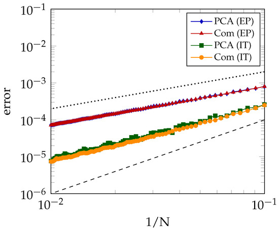
Figure 1.
Error with respect to the semidiscrete values for and if . Two reference lines included for first-order convergence (dotted) and second-order convergence (dashed).
Let as above. Table 1 displays our reference values for the PCA-based and comonotonic approximations and , respectively, as well as the lower bound for the European basket put option. These values have been obtained by applying the PDE discretisation from Section 3 with spatial and temporal grid points. Clearly, the positive result holds that, for each given set, the two approximations and the lower bound lie close to each other.

Table 1.
Reference values , , for European basket put option.
Similarly, Table 2 shows our reference values for , , for the American basket put option. These values have been obtained by applying the PDCP discretisation from Section 3 and . We find the favourable result that also in the American case, for each given set, the PCA-based and comonotonic approximations lie close to each other. Recall that, at present, it is not clear whether forms an actual lower bound in this case.
Table 2.
Reference values , , for American basket put option.
We next study, for European and American basket put options and Sets A–F, the absolute error in the discretisation described in Section 3 of the PCA-based and comonotonic approximations and in function of . To determine the error of the discretisation for the PCA-based and comonotonic approximations, the corresponding reference values from Table 1 and Table 2 are used.
Figure 2 and Figure 3 display for Sets A, B, C and D, E, F, respectively, the absolute error in the discretisation of and versus , where the left column concerns the European option and the right column the American option.
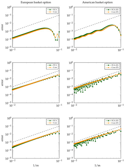
Figure 2.
Discretisation error for and in cases A (top), B (middle) and C (bottom). Left: European basket option. Right: American basket option. Reference line (dashed) included for second-order convergence.
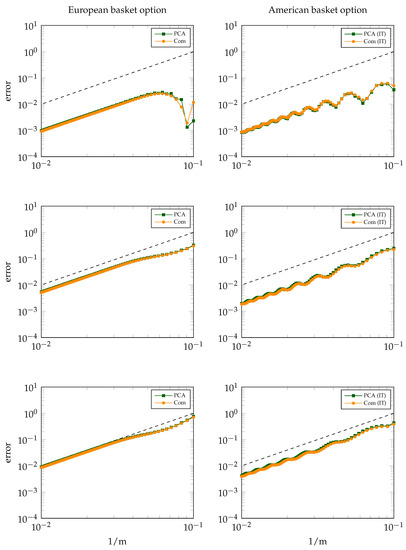
Figure 3.
Discretisation error for and in cases D (top), E (middle) and F (bottom). Left: European basket option. Right: American basket option. Reference line (dashed) included for second-order convergence.
As a main observation, Figure 2 and Figure 3 clearly indicate (near) second-order convergence of the discretisation error in all cases, that is, for all Sets A–F, for both the European and American basket options, and for both the PCA-based and comonotonic approximations. This is a very favourable result. Additional experiments indicate that the error stems essentially from the spatial discretisation (and not the temporal discretisation).
For the European option and Sets A and D, we remark that the error drop in the (less important) region corresponds to a change of sign. Besides this, in the case of the European basket option, the behaviour of the discretisation error is always seen to be regular.
For the American option, it is found that the discretisation error often behaves somewhat less regular, with oscillations occurring. A similar phenomenon has recently been observed and studied in [5] for Bermudan basket options and is attributed to the spatial nonsmoothness of the exact option value function at the early exercise boundary.
In the following we consider the second part of experiments and choose parameter sets inspired by those from [13]. Here a basket put option with equally weighted underlying assets is taken and . Next, the strike and the maturity time . For the interest rate we choose (this differs from [13] where the rate is taken, but then American option values are often close to their European counterpart, which is less interesting). Finally, the volatilities are given by
with . We select correlation for all . Then, for the pertinent two covariance matrices, the first eigenvalue is dominant. In particular, there holds
Further, the relevant matrices of eigenvectors Q satisfy the assumption from Section 2.1.
Table 3 and Table 4 show our reference values for , , for the European and American basket put option, respectively, which have been obtained in the same way as above. Again, we find the favourable result that, for each given parameter set and each given (European or American) option, these three values lie close to each other.
Table 3.
Reference values , , for European basket put option.
Table 4.
Reference values , , for American basket put option.
Figure 4 displays, analogously to Figure 2 and Figure 3, the absolute error in the discretisation of and for the (representative) three parameter sets given by , , . The outcomes again indicate a favourable, second-order convergence result. The regularity of the error behaviour is seen to decrease as the maturity time T increases. We note that for this behaviour is partly explained from a (near) vanishing error when .
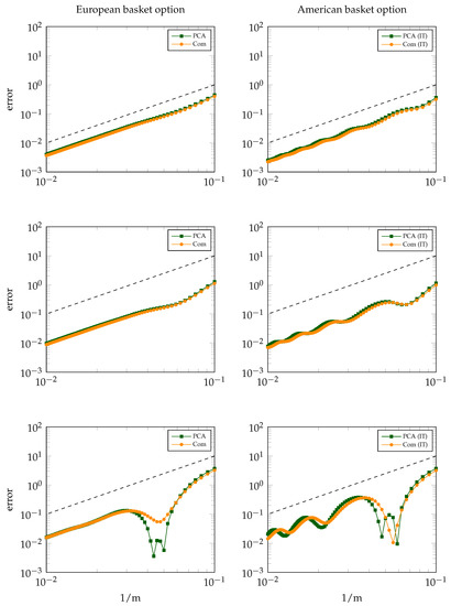
Figure 4.
Discretisation error for and in cases (top), (middle) and (bottom) where , . Left: European basket option. Right: American basket option. Reference line (dashed) included for second-order convergence.
6. Conclusions
The valuation of American basket options via d-dimensional PDCPs constitutes a notoriously challenging task whenever the number of assets d is medium or large. In this paper, we have studied an extension of the PCA-based approach by Reisinger and Wittum [1] to valuate American basket options. This approximation approach is highly effective, as the numerical solution of only a limited number of low-dimensional PDCPs is required. In addition, we have considered the comonotonic approach, which was developed for basket options notably in [6,7,8,9,10,11,12,19]. We have studied the comonotonic approximation formula for American basket option values recently examined in Hanbali and Linders [13]. The comonotonic approach is also highly effective, since it requires the numerical solution of just two one-dimensional PDCPs. To our knowledge, the present paper is the first in the literature where these two, different but related, approaches are jointly investigated.
For the discretisation of the pertinent PDCPs, we apply finite differences on a nonuniform spatial grid followed by the Brian and Douglas ADI scheme on a uniform temporal grid and selected the Ikonen–Toivanen (IT) technique [15,16,17] to efficiently handle the complementarity problem in each time step.
As a first main result, we find in ample numerical experiments that the PCA-based and comonotonic approaches always yield approximations to the value of an American (as well as European) basket option that lie close to each other.
As a next main result, we observe near second-order convergence of the discretisation error in all numerical experiments for both the PCA-based and comonotonic approaches for American (as well as European) basket options.
At this moment it is still open which (if any) of the two approaches, PCA-based or comonotonic, is to be preferred for the approximate valuation of American basket options on assets. In particular, whereas in our experiments the two approaches always define approximations that lie close to each other, it is not clear at present which approach (if any) generally yields the smallest error with respect to the exact option value. The comonotonic approach requires less computational work than the PCA-based approach, but both are computationally cheap.
A further investigation into the PCA-based and comonotonic approaches, both experimental and analytical, will be the subject of future research. This concerns the open question above as well as their fundamental properties, such as convergence, and their range of applications.
The following abbreviations are used in this manuscript:
Author Contributions
Methodology, K.J.i.H. and J.S.; software, K.J.i.H. and J.S.; investigation, K.J.i.H. and J.S.; writing—original draft preparation, K.J.i.H. and J.S.; supervision, K.J.i.H. All authors have read and agreed to the published version of the manuscript.
Funding
This research received no external funding.
Institutional Review Board Statement
Not applicable.
Informed Consent Statement
Not applicable.
Data Availability Statement
Restrictions apply to the availability of these data.
Conflicts of Interest
The authors declare no conflict of interest.
References
- Reisinger, C.; Wittum, G. Efficient hierarchical approximation of high-dimensional option pricing problems. SIAM J. Sci. Comp. 2007, 29, 440–458. [Google Scholar] [CrossRef]
- Reisinger, C.; Wissmann, R. Numerical valuation of derivatives in high-dimensional settings via partial differential equation expansions. J. Comp. Finan. 2015, 18, 95–127. [Google Scholar] [CrossRef]
- Reisinger, C.; Wissmann, R. Error analysis of truncated expansion solutions to high-dimensional parabolic PDEs. ESAIM M2AN 2017, 51, 2435–2463. [Google Scholar] [CrossRef][Green Version]
- Reisinger, C.; Wissmann, R. Finite difference methods for medium- and high-dimensional derivative pricing PDEs. In High-Performance Computing in Finance: Problems, Methods, and Solutions; Chapman and Hall/CRC: London, UK, 2018; pp. 175–196. [Google Scholar]
- in ’t Hout, K.; Snoeijer, J. Numerical valuation of Bermudan basket options via partial differential equations. Int. J. Comp. Math. 2021, 98, 829–844. [Google Scholar] [CrossRef]
- Kaas, R.; Dhaene, J.; Goovaerts, M. Upper and lower bounds for sums of random variables. Insur. Math. Econ. 2000, 27, 151–168. [Google Scholar] [CrossRef]
- Dhaene, J.; Denuit, M.; Goovaerts, M.; Kaas, R.; Vyncke, D. The concept of comonotonicity in actuarial science and finance: Theory. Insur. Math. Econ. 2002, 31, 3–33. [Google Scholar] [CrossRef]
- Dhaene, J.; Denuit, M.; Goovaerts, M.; Kaas, R.; Vyncke, D. The concept of comonotonicity in actuarial science and finance: Applications. Insur. Math. Econ. 2002, 31, 133–161. [Google Scholar] [CrossRef]
- Deelstra, G.; Liinev, J.; Vanmaele, M. Pricing of arithmetic basket options by conditioning. Insur. Math. Econ. 2004, 34, 55–77. [Google Scholar] [CrossRef]
- Deelstra, G.; Diallo, I.; Vanmaele, M. Bounds for Asian basket options. J. Comp. Appl. Math. 2008, 218, 215–228. [Google Scholar] [CrossRef][Green Version]
- Chen, X.; Deelstra, G.; Dhaene, J.; Vanmaele, M. Static super-replicating strategies for a class of exotic options. Insur. Math. Econ. 2008, 42, 1067–1085. [Google Scholar] [CrossRef][Green Version]
- Chen, X.; Deelstra, G.; Dhaene, J.; Linders, D.; Vanmaele, M. On an optimization problem related to static super-replicating strategies. J. Comp. Appl. Math. 2015, 278, 213–230. [Google Scholar] [CrossRef]
- Hanbali, H.; Linders, D. American-type basket option pricing: A simple two-dimensional partial differential equation. Quant. Fin. 2019, 19, 1689–1704. [Google Scholar] [CrossRef]
- in ’t Hout, K. Numerical Partial Differential Equations in Finance Explained; Financial Engineering Explained; Palgrave Macmillan: London, UK, 2017. [Google Scholar]
- Haentjens, T.; in ’t Hout, K. ADI schemes for pricing American options under the Heston model. Appl. Math. Fin. 2015, 22, 207–237. [Google Scholar] [CrossRef]
- Ikonen, S.; Toivanen, J. Operator splitting methods for American option pricing. Appl. Math. Lett. 2004, 17, 809–814. [Google Scholar] [CrossRef]
- Ikonen, S.; Toivanen, J. Operator splitting methods for pricing American options under stochastic volatility. Numer. Math. 2009, 113, 299–324. [Google Scholar] [CrossRef]
- in ’t Hout, K.; Valkov, R. Numerical Study of Splitting Methods for American Option Valuation. In Novel Methods in Computational Finance; Springer: Berlin/Heidelberg, Germany, 2017; pp. 373–398. [Google Scholar]
- Vyncke, D.; Goovaerts, M.; Dhaene, J. An accurate analytical approximation for the price of a European-style arithmetic Asian option. Finance 2004, 25, 121–139. [Google Scholar]
- Jain, S.; Oosterlee, C. The stochastic grid bundling method: Efficient pricing of Bermudan options and their Greeks. Appl. Math. Comp. 2015, 269, 412–431. [Google Scholar] [CrossRef]


Publisher’s Note: MDPI stays neutral with regard to jurisdictional claims in published maps and institutional affiliations. |
© 2021 by the authors. Licensee MDPI, Basel, Switzerland. This article is an open access article distributed under the terms and conditions of the Creative Commons Attribution (CC BY) license (https://creativecommons.org/licenses/by/4.0/).