Abstract
Fractional-order time and space derivatives are one way to augment the classical diffusion equation so that it accounts for the non-Gaussian processes often observed in heterogeneous materials. Two-dimensional phase diagrams—plots whose axes represent the fractional derivative order—typically display: (i) points corresponding to distinct diffusion propagators (Gaussian, Cauchy), (ii) lines along which specific stochastic models apply (Lévy process, subordinated Brownian motion), and (iii) regions of super- and sub-diffusion where the mean squared displacement grows faster or slower than a linear function of diffusion time (i.e., anomalous diffusion). Three-dimensional phase cubes are a convenient way to classify models of anomalous diffusion (continuous time random walk, fractional motion, fractal derivative). Specifically, each type of fractional derivative when combined with an assumed power law behavior in the diffusion coefficient renders a characteristic picture of the underlying particle motion. The corresponding phase diagrams, like pages in a sketch book, provide a portfolio of representations of anomalous diffusion. The anomalous diffusion phase cube employs lines of super-diffusion (Lévy process), sub-diffusion (subordinated Brownian motion), and quasi-Gaussian behavior to stitch together equivalent regions.
1. Introduction
Fractional calculus (non-integer order integration and differentiation) extends the local, memory-free concepts of Newton and Leibniz [1,2], but this growth entails a mosaic of non-integer derivatives whose diverse properties can overwhelm new users. Given the long history and distinguished pedigree of fractional calculus [3,4], one would think that by now it would have an established niche in mathematical physics (as have generalized functions and pseudo-differential operators [5]). Nevertheless, while widely used in electrochemistry, viscoelasticity, dielectric relaxation and anomalous diffusion, the tools of fractional calculus are often overlooked. This paradox suggests that we search for new ways to introduce the multiple forms of fractional-order derivatives (Grünwald–Letnikov, Riemann–Liouville, Caputo, Riesz–Weyl, etc.) to new investigators seeking to apply fractional calculus in their research.
In the field of magnetic resonance imaging (MRI), this question can be focused on the Bloch–Torrey equation [6], and on the selection of the proper fractional-order tools for generalizing relaxation and diffusion phenomena that occur in complex biological tissues. Incorporation of a fractional time derivative into a first order relaxation equation yields a single parameter Mittag–Leffler function that enhances the integer-order exponential decay model [7], while employing a fractional space derivative in the classical diffusion equation provides a stretched exponential solution that expands the Gaussian model to one of Lévy motion [8]. Selection of a particular fractional derivative for each case is based on anticipating how material composition, heterogeneity and, in some cases, fractal structure might be incorporated into the analysis [9,10].
What can guide the researcher in choosing one fractional derivative over another? When should the material parameters in the models be constants or functions of position and time? Why use only a linear model? These questions quickly take us beyond the scope of the current paper but provide context for this investigation. Specifically, here we will examine fractional-order models that generalize the classical Gaussian solution to the diffusion equation as it is encountered in MRI. The goal is not to apply a particular model to a given set of data, but to compare and contrast different models (e.g., integer-order, fractional-order; linear, non-linear; constant diffusion coefficients, variable diffusion coefficients). The comparison tool we have chosen will be a scaling analysis of the governing one-dimensional diffusion equation. We will illustrate the results using a phase diagram as a means of classifying the time-dependence of the mean-squared displacement of the underlying random motion. We will illustrate the behavior of each model by presenting the phase diagram as an orthogonal slice of a three-dimensional anomalous diffusion phase cube. Lines of super-diffusion (Lévy process) and sub-diffusion (subordinated Brownian motion, fractional Brownian motion, etc.) for each two-dimensional phase diagram will be seen to link different diffusion models—displaying corresponding regions of sub- and super-diffusion.
2. Background
There are now available more than one hundred books on fractional calculus, each describing specific aspects of the formulation, properties and applications of fractional derivatives in physics, chemistry, biology, and engineering (https://mechatronics.ucmerced.edu/fcbooks) (accessed on 20 May 2021). An annotated bibliography of books that we have found useful can be found in Chapter XII of the book, Fractional Calculus in Bioengineering [4]. In addition, for reference, the definitions and basic properties of the fractional operators used in this paper are listed in the Supplementary Materials (Tables S1 and S2) of this paper. These tables and Appendix A and Appendix B of this paper should help researchers who are not familiar with specific properties of different forms of fractional integration and differentiation.
In addition, it is an inconvenient truth that the Greek letters often used in fractional calculus to indicate, non-integer, fractional-order operations (α, β, γ, …) are not applied in a consistent manner for time and space derivatives but shift with the author’s preference and historical precedent. Since Jeremy Bentham’s ‘calculus of felicity’ (https://plato.stanford.edu/entries/) (accessed on 20 May 2021) is not part of fractional calculus, the operator notation in fractional calculus was not formulated to keep all users happy; hence, we must be ever wary of the local terminology. It should also be kept in mind that interchanging operations between fractional and integer-order calculus should be viewed with suspicion; one should not mix the tools and notation together any more carelessly than trying to assemble a motor using parts with both metric and British Standard Whitworth threads [11]. Consequently, in the results below we will employ a restricted set of fractional derivatives and identify the local notation in a consistent manner for each case.
3. Results
In this section two groups of fractional order diffusion equations, Section 3.1 and Section 3.2, are considered where β, denotes the order of the fractional time derivative, and α, indicates the order of the fractional space derivative. In the first group, Section 3.1, Table 1, we assume a linear diffusion equation with a diffusion coefficient that is a power law function of time, , where . The general solution for each of these equations can be expressed in terms of the Fox, H-function [10], and its Fourier transform has been used to model diffusion studies in MRI [12]. In the second group, Section 3.2, Table 2, we assume both linear and non-linear fractional order models of diffusion with a diffusion coefficient that is a power law function of both space and time, , where and . The general solution for this group is not available in a closed form and, only a few special cases have been used in MRI. For both groups we use scaling principles [13] to determine the mean squared displacement (MSD) for a multi-dimensional, Euclidean phase space, . Two-dimensional phase diagrams of each model are displayed, for convenience, as a slice of a three-dimensional anomalous phase cube, e.g., or . The MSD appears as a line of quasi-Gaussian behavior on the phase diagram separating regions of sub- and super-diffusion.

Table 1.
Anomalous diffusion with power law diffusion coefficient, .
Table 2.
Anomalous diffusion with power law diffusion coefficient, .
In the first group of equations, Section 3.1, we describe linear fractional time and space diffusion where the diffusion coefficient is assumed to vary as function of time, . The first diffusion example (Section 3.1.1) describes the floor of the phase cube as a two-dimensional phase diagram , for fractional time and space derivatives with a constant diffusion constant, , with dimensions, . The next two cases describe faces of the phase cube that intersect the fractional derivative floor along the line (fractional motion, Section 3.1.2), and along the line (fractional Kilbas–Saigo decay, Section 3.1.3). In both cases the diffusion coefficient varies with time as a power law.
In the second group of equations, Section 3.2, we describe linear fractional time diffusion with linear and non-linear space diffusion of degree, , where the diffusion coefficient is assumed to vary as function of space and time, . The first example (Section 3.2.1) is linear, , with , and describes the phase cube . The next example (Section 3.2.2) is a non-linear model of diffusion with a power law space diffusion coefficient, , and describes the phase cube . The last example (Section 3.2.3) is a linear diffusion model with a fractional order time and an integer order space derivative, and a diffusion coefficient that varies as a power law in both space and time, , so that corresponding to the phase polytope is a tesseract .
In the following, the diffusion equation will be described in terms of the particle density, P(x,t), with the units of , where the particle can be a molecule a microbe, or any object whose physical size is small compared to its surroundings.
3.1. Fractional Time and Space Derivatives with Power Law D(t)
Consider the one-dimensional fractional diffusion equation of P(x,t) that includes a time-varying power law diffusion coefficient with the Caputo time and symmetric Riesz space derivatives:
Here, the order of symmetric Riesz space derivative is α, (), the order of the Caputo time derivative is β, (), and the Greek letter ν, () is assigned to the assumed power law dependence of diffusion coefficient. The diffusion coefficient in this case is a constant, , multiplying . The units of are . The solution to Equation (1) for an initial value problem with a Dirac delta function concentration of material at the origin of an unbounded domain, is given in Appendix A.2. The result can be written as an inverse Fourier transformation of the Kilbas–Saigo function,
If we assume that Equation (2) can be written in the scaled form,
with , [14,15,16], then the corresponding mean squared displacement (MSD) is:
with for , where may not exist for all values of and (See Appendix A.1 for details). Analyzing the time behavior of the mean squared displacement in Equation (4) leads us to recognize sub-diffusion, normal diffusion, and super-diffusion when: , , and , respectively. The three fractional parameters of the anomalous phase cube {} describe: (i) Gaussian diffusion with a power law , (ii) fractional time and space diffusion (FTS) with a power law , (iii) fractional space diffusion (FS) with a power law , and (iv) fractional time diffusion (FT) with a power law , models of anomalous diffusion—all subsumed by Equation (1)—and displayed with the corresponding power law time-dependence of the MSD in Table 1.
Equation (1) has three separate power law relationships, two ( arising from the CTRW model (inverse power law tails of waiting times, , , and jump increments, , ) [17], and one coming from the power-law time behavior, , in the diffusion coefficient. An overview of regions of sub- and super-diffusion is displayed in Figure 1 as slices of the phase cube. When this is the fractional calculus model of anomalous diffusion, case (Section 3.1.1), when it becomes the fractional motion model, case (Section 3.1.2), and when it is the fractional power law model, case (Section 3.1.3). Each case will be briefly described below.
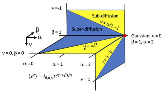
Figure 1.
Three faces of the phase cube are shown in this figure. Each face corresponds to the situation where one of the fractional parameters is fixed: and . The faces are divided by diagonal lines along which the mean squared displacement is a linear function of time (quasi-Gaussian diffusion). The regions of sub- and super-diffusion are displayed in yellow and blue, respectively.
3.1.1. Diffusion Equation with Fractional Time and Space Derivatives
The continuous time random walk (CTRW) model of anomalous diffusion is widely used because it provides a direct connection between the statistical properties of particle trapping and jump increments (inverse power laws) with the order of the time and space fractional derivatives in the associated diffusion equation [17,18].
Consider the one-dimensional diffusion equation for the CTRW model of P(x,t) expressed in terms of fractional time and space derivatives:
Here, the Greek letter , (), is used to designate the order of Caputo fractional time derivative, while the Greek letter , (), is used to designate the order of the symmetric Riesz fractional space derivative (both derivatives are defined in Supplementary Tables S1 and S2). The diffusion coefficient in this case, , is a constant, and has the units of .
The solution to Equation (5) when all particles are initially concentrated at the origin of an unbounded domain, , is a Fox, H-function [19,20], which can be written as:
where for we have,
The corresponding MSD is formally given by:
where , with the understanding that the MSD does not exist for the entire range of the fractional order parameters. Analyzing the behavior of the in Equation (8) leads us to recognize sub-diffusion, normal diffusion, and super-diffusion when: , , and , respectively.
The Fourier transformation of Equation (6), can be expressed as a one-parameter Mittag–Leffler function [20]:
This solution, which is the characteristic function of the P(x,t), also describes the time decay of each spatial frequency of the associated random motion. It yields particular cases for selected values of the fractional derivatives: Gaussian (), Lévy process (), and subordinated Brownian motion for (). These special cases of anomalous diffusion for the CTRW model are displayed in Figure 1 as a two-dimensional phase diagram. This phase diagram corresponds with the plane of the anomalous phase cube {} in Figure 1.
3.1.2. Integer Time Derivative and Fractional Space Derivative with Power Law D(t)
This anomalous diffusion model was defined by Eliazar and Shlesinger as ‘fractional motions’ [21]. It differs from the CRTW model by allowing persistence and anti-persistence in the jump increments of particle motion. This behavior is incorporated into a modified fractional diffusion equation by setting the order of the time derivative, , and introducing a time-dependent diffusion coefficient, which is assumed to be a power law. Eliazar and Shlesinger provide a complete description of this extended model of Brownian motion in [21] where the rare extremes of large jumps is described as the Noah exponent (α in our notation), while persistence, or anti-persistence of motion is characterized as the Joseph exponent (ν in our notation). They also show its connection to Lévy motion and the Hurst exponent (H). The utility of this diffusion model in MRI is illustrated by Fan and Gao [22] and by Karaman et al. [23,24].
Consider the one-dimensional diffusion equation for the fractional motions model of P(x,t) expressed in terms of the integer time derivative and fractional space derivative:
Here, the Greek letter , () is used to designate the order of the symmetric Riesz fractional space derivative, while the Greek letter , () is the assumed power law dependence of the time-dependent diffusion coefficient, . The diffusion coefficient in this case includes a constant, multiplying , where has the units of .
The solution to Equation (10) for an initial concentration of material at the origin of an unbounded domain is a fractional Lévy motion [21] can be written as:
where for we have,
The corresponding mean squared displacement is:
with , with the understanding that the MSD does not exist for the entire range of the fractional order parameters The Fourier transformation of Equation (11), has a simple stretched exponential solution:
This solution describes the time decay of each spatial frequency component. It yields particular cases for selected values of the fractional derivatives: Gaussian (), Cauchy (), Levy process ), and fractional Brownian motion for ). The governing diffusion equations for these cases are shown in the Supplementary Table S3.
Classification of this behavior in terms of sub- and super-diffusion in the plane is displayed in Supplementary Table S4. The MSD is expressed in terms of the Hurst fractal dimension (H) of the diffusion trajectory as , with This expression corresponds to quasi-diffusion (QD) when , H = ½, super-diffusion when 1/α < H < 1, and sub-diffusion when 0 < H < 1/α. This phase diagram corresponds with the plane on the back side of the anomalous phase cube {}, in Figure 1.
3.1.3. Fractional Time Derivative and Integer Space Derivative with Power Law D(t)
The fractional power law model complements the ‘fractional motions’ model by assuming a fractional time derivative, β, , but with the order of the space derivative, . In the context of the CTRW model, particle trapping is proscribed, while jump increments must have a finite second moment. Introducing a time-dependent diffusion coefficient provides an independent time-scaling parameter, one that has been associated with fractal properties of the medium [fractal/fractional model]. A complete description of this extended model of Brownian motion and its connection to CTRW motion is provided by Gorenflo et al. in [7]. The utility of this diffusion model in MRI is illustrated by Fan and Gao [22] and by Magin et al. [12].
Consider the one-dimensional diffusion equation of P(x,t) with a power law expressed in terms of a fractional time and an integer space derivative:
Here, the order of space derivative, α, is set to two, the order of the Caputo time derivative is β, (), and the Greek letter ν, () is assigned to the assumed power law dependence of diffusion coefficient. The diffusion coefficient in this case is a constant, , multiplying . The units of are . The solution, P(x,t), for an initial concentration of material at the origin of an unbounded domain is a Kilbas–Saigo function [10] (p. 21):
which may also be written as:
with,
The corresponding mean squared displacement is:
with for with the understanding that the MSD does not exist for the entire range of the fractional order parameters.
The Fourier transformation of Equation (17), is a Kilbas–Saigo function:
The Kilbas–Saigo function is a special form of the three parameter Mittag–Leffler function [20] that includes the exponential ( stretched single parameter Mittag–Leffer (), and stretched exponential () functions as special cases. The governing diffusion equations for these cases are shown in the Supplementary Table S5.
Classification of this behavior in terms of sub- and super-diffusion in the plane is displayed in Figure 1. The mean squared diffusion for this model of anomalous diffusion has a time dependence of the form . This expression corresponds to quasi-diffusion when , super-diffusion when , and sub-diffusion when . This phase diagram corresponds with the plane on the right side of the anomalous phase cube {} in Figure 1.
3.2. Fractional Time and Space Derivatives with Power Law D(x,t) and Non-Linear in P(x,t)
The classical derivation of the diffusion equation is a combination of a flux defined as the negative gradient of particle concentration, , where D is the diffusion constant (), with a continuity equation , which yields the diffusion equation in one dimension: [25]. Extending this derivation using fractional calculus suggests—in addition to introducing fractional operators for the time and space derivatives—that one might have reason to modify either the flux or the continuity equation (or both) [26,27]. This approach also introduces the notion of sequential fractional space derivatives [1,3], and the possibility of inserting a space or time dependent diffusion coefficient in the definition of the diffusion coefficient [10], as well as the possibility of a non-linear flux. Although the last step might seem arbitrary, it is consistent with the porous media model of the diffusion equation [28], the extension of diffusion from one to n dimensions [29], the characterization of diffusion across fractal interfaces [30], and the description of porous materials in terms of fractal dimensions [31]. In this section we will investigate a linear/non-linear model that describes fractional diffusion combined with an inverse power law time and space dependence diffusion coefficient.
Consider the one-dimensional, non-linear, fractional diffusion equation of P(x,t) that includes a time- and space-varying power law diffusion coefficient with the Caputo time and symmetric Riesz space derivatives:
Here, the order of symmetric Riesz space derivative is α, (), the order of the Caputo time derivative is β, (), [10], where , is a positive real number, while the Greek letter , (), is the degree of , and has the units of .
The general solution to Equation (21) for an initial value problem with a Dirac delta function concentration of material at the origin of an unbounded domain, is not available. If we assume that the normalized solution to Equation (21) can be written in the scaled form:
then by the approach used in [32,33] we find (Appendix B.1), .
The corresponding mean squared displacement (MSD) is:
where for and with the understanding that the MSD does not exist for the entire range of the fractional order parameters (see Appendix B.1 and [16] (Chapter 16) for details).
Analyzing the time behavior of the mean squared displacement in Equation (23) leads us to recognize sub-diffusion, normal diffusion, and super-diffusion when: , 2, and , respectively. In Table 2 we display special cases of Equation (21) that will be considered further: (i) linear anomalous diffusion with a power law, , in Section 3.2.1, (ii) non-linear anomalous diffusion with a power law diffusion coefficient, , in Section 3.2.2, and (iii) linear anomalous diffusion with a time- and space-varying diffusion coefficient, , in Section 3.2.3.
3.2.1. Fractional Time and Space Derivatives with Power Law, D(x), and Linear in P(x,t)
Consider the one-dimensional fractional diffusion equation of P(x,t) that includes a space-varying power law diffusion coefficient with the Caputo time and symmetric Riesz space derivatives:
The corresponding mean squared displacement is:
Here, the Greek letter, , (), is the order of the Caputo fractional time derivative, and the Greek letter , (), is the order of the symmetric Riesz fractional space derivative. The diffusion coefficient in this case, , is a constant and has the units of . The general solution to Equation (24) is not known. Solutions of this equation for an initial concentration of material at the origin of an unbounded domain are presented for specific cases in [10] and Appendix B.2.
For example, when , the integer order solution to Equation (24) is a stretched exponential [34,35]:
The corresponding mean squared displacement is:
Both Equations (26) and (27) condense to the Gaussian case when . When the MSD displays sub- and super-diffusion for , and for , respectively.
For the case, when all particles are initially concentrated at the origin, , the solution to Equation (24) in an unbounded domain is a Fox, H-function [36] (Appendix B.2), which can be written as:
where,
with , and,
In the general case, this model fills the anomalous phase cube {} with regions of sub- and super-diffusion that correspond to the situations where the exponent of the MSD, , is less than or greater than one. Classification of this behavior in terms of sub- and super-diffusion is displayed in Figure 2.
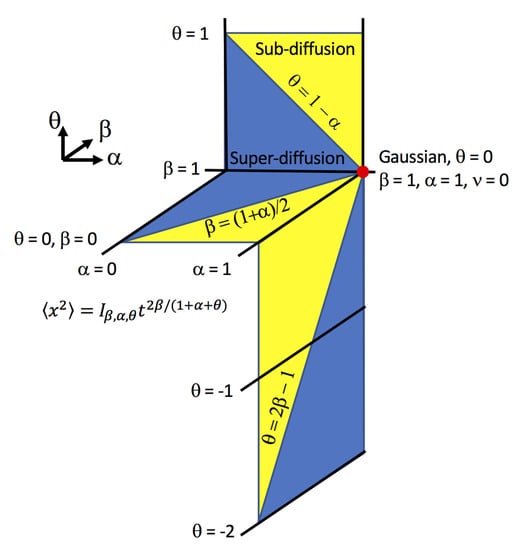
Figure 2.
Three faces of the phase cube are shown in this figure. Each face corresponds to the situation where one of the fractional parameters is fixed: , and . The faces are divided by diagonal lines along which the mean squared displacement is a linear function of time. Regions of sub- and super-diffusion are displayed in yellow and blue, respectively.
When , the super-diffusion domain of the plane merges with the fractional diffusion model (Lévy motion), while also for the sub-diffusion domain of the plane merges with the fractional diffusion model (subordinated Brownian motion). When , the vertical line, reflects the stretched exponential solution for , which is Gaussian for , and exhibits sub-diffusion when is positive and super-diffusion when is negative.
3.2.2. Integer Time Derivative with a Non-Linear Space Derivative and a Power Law D()
Diffusion in complex materials has been modeled using a non-linear version of the classical diffusion equation (porous media equation) where P(x,t) is raised to a power, ρ [37,38,39]. In this section we will outline the fractional order generalization of this non-linear model, largely following the work described in [37,39], and in Chapter 6 of the book on fractional diffusion equations and anomalous diffusion by Evangelista and Lenzi [10].
Consider the one-dimensional non-linear fractional diffusion equation for P(x,t) expressed in terms of the symmetric Riesz space derivative and a power law diffusion coefficient :
The corresponding mean squared displacement is derived from a scaling argument in Appendix B.3:
with for , and with the understanding that the MSD does not exist for the entire range of the fractional order parameters. Here the order of the fractional space derivative, is (), is a positive real number, and the range of the fractional power is (). The diffusion constant, has the units .
Using the scaling argument in Appendix B.3, and expressing in terms of with , as:
it is possible to simplify Equation (31) as:
For an initial concentration of material at the origin of an unbounded domain particular solutions to Equation (34) are [38]:
For the case of , and
in the case of , with
where and are a normalization factors, and a and b are chosen such that Equation (36) satisfies Equation (34). The parameter is chosen , depending on the behavior of the solution. In fact, for a compact behavior, we have and for a long-tailed behavior . Note that the solutions shown for the non-linear case are given in terms of power laws and may be related to the Levy distributions as discussed in [10,37,38,39].
In the general case, this model fills the anomalous phase cube {} with regions of sub- and super-diffusion that correspond to the situations where the exponent of the MSD, , is less than or greater than one. Classification of this behavior in terms of sub- and super-diffusion is displayed in Figure 3, which is one of the eight phase cubes that comprise the {} tesseract.
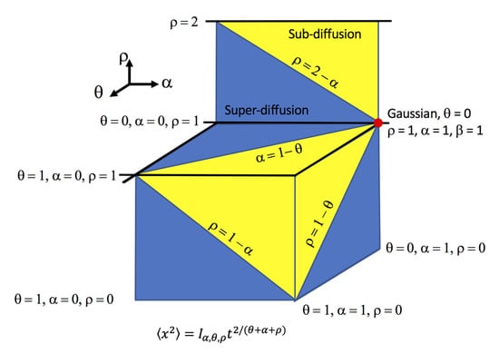
Figure 3.
Four faces of the phase cube are shown in this figure. Each face corresponds to the situation where one of the fractional parameters is fixed: , , , and . The faces are divided by diagonal lines along which the mean squared displacement is a linear function of time. Regions of sub- and super-diffusion are displayed in yellow and blue, respectively.
In Figure 3, the linear model of anomalous diffusion is displayed as the top of a phase cube (, as a two-dimensional , phase diagram that is divided into regions of super- and sub-diffusion by the line, , with the Gaussian diffusion case at the point . The plane is intersected by the and the planes illustrating complementary phase behavior for the non-linear model when . For the plane, the line of quasi-diffusion (, where the MSD is proportional to diffusion time), also has a negative slope when . Finally, the , , and planes slice off a corner of subdiffusion from the phase cube .
3.2.3. Fractional Time Derivative and Integer Space Derivatives with a Time and Space-Dependent Diffusion Coefficient, and Linear in P(x,t)
Consider the one-dimensional linear diffusion equation for P(x,t), with integer space derivatives and a Caputo time derivative, , ():
The corresponding mean squared displacement is derived from a scaling argument in Appendix B.4:
where for with the understanding that the MSD does not exist for the entire range of the fractional order parameters.
Here, the diffusion coefficient in this case, is a constant and has the units of . Solutions of this equation for an initial concentration of material at the origin of an unbounded domain are presented for specific cases (additional cases can be found in [10]).
The general solution to Equation (38) for an initial concentration of material at the origin of an unbounded domain [40] is derived in Appendix B.4 using:
with
In this case, the model reflects the anomalous phase cube {} with regions of sub- and super-diffusion that correspond to the situations where the exponent of the MSD, (, is less than or greater than one. Classification of this behavior in terms of sub- and super-diffusion is displayed in Figure 4, which is one of the eight phase cubes that comprise the {} tesseract.
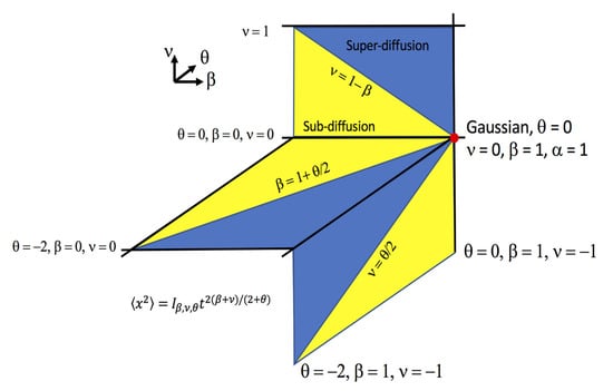
Figure 4.
Three faces of the phase cube are shown in this figure. Each face corresponds to the situation where one of the fractional parameters is fixed: , , and . The faces are divided by diagonal lines along which the mean squared displacement is a linear function of time. Regions of sub- and super-diffusion are displayed in yellow and blue, respectively.
In Figure 4, the linear model of anomalous diffusion is displayed on the top face of a phase cube , as a two-dimensional , phase diagram that is divided into regions of super- and sub-diffusion by the line, , with the Gaussian diffusion case appearing at the point . The plane is intersected by the plane and the plane (where the MSD does not exist). For the plane, the line of quasi-diffusion (, where the MSD is proportional to diffusion time), shows a negative slope when . Finally, the , and , planes slice off a wedge of sub-diffusion from the phase cube , while the , and , planes slice off a wedge of super-diffusion.
4. Discussion
The phase diagrams displayed in the results section (Figure 1, Figure 2, Figure 3 and Figure 4) depict models of anomalous diffusion (Table 1 and Table 2) as a slice of a three or n-dimensional solid (anomalous phase hypercube). The intent of this representation is to provide a perspective that connects the underlying mathematical models (fractional diffusion equations) with the expected regions of sub- and super-diffusion. Our overall goal is to present these diagrams as an aid in the interpretation of diffusion data collected from porous, heterogeneous material, such as, that acquired in diffusion-weighted MRI experiments.
Anomalous diffusion, typically characterized by asymptotic, power law tails for and a power law growth in time of the mean squared displacement (MSD) [41], sprouts from the deep root of Brownian motion in its many variegated forms. Here we classify these forms by comparing the power law exponent (R) of the MSD for each model () with the classical result for Brownian motion (, where R = ½). In Section 3.1, we combine the CTRW model of anomalous diffusion with a power-law form of the time-dependent diffusion coefficient, . For this model, Equation (1), we show that the MSD can be obtained directly from the analytical solution of specific cases (using Fox, H-functions) as well as from a scaling analysis of the governing fractional order differential equation (details in Appendix A). The results include the special cases of Lévy motion, fractional motion and subordinated fractional diffusion.
In Section 3.2, we consider a modified CTRW model of anomalous diffusion derived by assuming a fractional flux gradient, , acting in concert with an integer order divergence term in the continuity equation. The resulting diffusion equation is also allowed to be non-linear, and to include a power-law time- and space-dependent diffusion coefficient, . For this model, Equation (21), we do not have an analytical solution for all cases but use scaling analysis (Appendix B.1) to obtain the MSD for three situations: first, a linear anomalous diffusion equation with a fractional time and a fractional space derivative, and (Section 3.2.1); second a non-linear anomalous diffusion equation with an integer time derivative, a fractional space derivative, and (Section 3.2.2); and finally a linear anomalous diffusion equation that uses a fractional time derivative, an integer order space derivative, and includes a time- and space-dependent power law diffusion coefficient (Section 3.2.3). The so-called porous medium equation appears under the umbrella of the non-linear case when both the time and space derivatives are of integer order [42].
Although each model springs from a different physical or mathematical perspective [43,44] (linear/non-linear, fractional/fractal, deterministic/stochastic, and constant/varying diffusion coefficient), its parameter space (order of the time and space derivatives, power-law exponents of the diffusion coefficients, degree of non-linearity and fractal dimensions) is divided into zones of sub- and super-diffusion by considering the behavior of the mean squared displacement for each model. In the phase cube representation, these zones coalesce to a point for the Gaussian behavior of Brownian motion, a line along which Lévy motion or subordinated Brownian motion appear, and a plane where regions of sub- and super-diffusion diffusion are displayed.
Phase diagrams are used throughout physics and engineering to map the behavior of physical systems [45]. Pressure–temperature, pressure–volume, temperature–volume (gases) and material composition (liquids and solids) phase diagrams are widely used in metallurgy and chemistry to guide our understanding of phase changes, optimization of fractional distillation, and chemical extraction procedures. General principles such as the Gibb’s phase rule (F = C − P + 2; the degrees of freedom of a system at equilibrium (F) is equal to the number of components (C) minus the number of phases (P) plus 2) guide the expected changes of state when the temperature, pressure or composition are varied. The idea is easily generalized to binary systems at constant pressure and to eutectic mixtures as well as to alloys and amalgams. In such cases slices of a multidimensional phase volume provide a means of organizing the complex material using multiple perspectives.
Chemical phase diagrams of single and multiple components (e.g., water, salt-water, lead-tin, iron-iron carbide) capture reams of experimental data (melting, vaporization, sublimation) in regions representing solid, liquid, and gaseous phases [46]. The molecular configuration in each phase is verified by microscopy and spectroscopy, and the diagrams modified to account for new phenomena (polymorphic solids, glasses, compressible liquids, and supercritical fluids). The result is not just an equilibrium description of the material at a fixed specific volume, but a road map showing how the terrain will change when experiments alter the temperature, pressure or composition. Implied, but not displayed in the phase diagram are the consequences of changing the temperature or pressure on the mobility and configurations of molecules.
Mathematical phase diagrams of fractional derivative orders (β time; and α, space) in the diffusion equation describe a myriad of analytical, numerical and Monte Carlo simulation results for the normal (Gaussian) and anomalous (Levy, fractional Brownian, subordinated, ballistic) motion of ideal particles [27,28]. The particle motion in each phase reflects an underlying material configuration where the mobility is characterized by sub-diffusion, super-diffusion, or quasi-Gaussian motion. Association of experimental measurements of ‘anomalous’ diffusion in a complex, heterogeneous material with a specific model using fitted values of β and α is not a one-to-one map of fractional derivative order to molecular configuration; it is doubly degenerate. First, at least in nuclear magnetic resonance (NMR) and MRI [47], because there are multiple sets of parameters that can with high fidelity match the observed data, and second because there are integer and fractional-order models of diffusion, some employing a power-law diffusion coefficient , which also fit the data.
Here, we would like to suggest several ways to combine these models. One idea is to overlap chemical and mathematical phase diagrams, beginning with simple materials. As an example, in Figure 5 we have superimposed a portion Figure 5 (e.g., the plane for fractional time and space diffusion with a constant coefficient) on the phase diagram of pure water [45] (triple point, tp, to critical point, cp,). Taking inspiration from the Clausius–Clapeyron equation [46], we associate //)] with the pressure ratio, and with the temperature ratio so that the critical point of the {P, T} diagram corresponds with the Gaussian point of the anomalous diffusion phase diagram. We then see that overlap of the phase diagrams divides the liquid and vapor phases of water into regions of putative sub- and super-diffusion, respectively. The combined diagram also suggests and that the supercritical fluid phase corresponds with the domain of Brownian motion in the mathematical phase diagram. This inchoate connection can perhaps be extended to other single- and multi-phase situations where anomalous diffusion or behavior appears. It also has the potential of linking chemical composition and material structure—for a given material—with the most appropriate slice of the phase cube and thus could provide a basis for selection of one model versus another. This correspondence might be extended by applying fractional calculus to theoretical models of the vapor–liquid equilibria (Chapter IX in [5,48]).
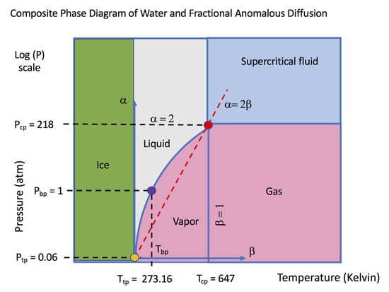
Figure 5.
Composite pressure-temperature {P, T} phase diagram of water with the fractional anomalous diffusion phase diagram. The critical point of water is taken to be equivalent with the Gaussian case of normal diffusion. In this example, the triple point of water appears near the origin of the anomalous diffusion diagram, while the boiling point is at the location, .
Alternatively, we can probe the underlying assumptions of kinetic, fractional order and stochastic models to establish how β and α reflect changes in kinetic theory concepts such as mean free path and the time between collisions with the CTRW probabilities of particle jumps and waiting times. The simplest compartmental representation of fractional derivatives is expressed in terms of a distribution of first order exponential decay processes. This approach, used by Berberan–Santos in luminescence studies [49], links lower order fractional derivatives with a broader distribution of compartments—a single compartment as the order approaches one. The CTRW model assumes particle jump and waiting time probabilities that by convolution embed material properties in the fractional order derivative operators. This correspondence was applied by Schumer and colleagues (see Figures 7 and 9 in [50]) to problems in erosion and groundwater contamination.
Classical diffusion theory links the time rate of change of particle concentration with the divergence of the flux, which is assumed to be proportional to the gradient of concentration. Here, we used the Caputo fractional time derivative to generalize the time rate of change and the symmetric Reisz fractional space derivative to generalize the flux (in Section 3.2, we have not modified the gradient operator in the continuity equation). The fractional time derivative affects particle dynamics by introducing memory in the time derivative, , while the fractional space derivative introduces non-locality, , [5,43]. Thus, memory and non-locality are introduced by convolution into mathematical physics when fractional order operators are employed.
Thinking of the classical diffusion problem as it might be affected by Maxwell’s demon—as William Thompson did in 1875 (see pages 57–60 in Reference [51])—the demon, is viewed as a batsman in cricket who sorts out pitches/particles entering a ‘control’ volume based on speed and direction. In the fractional calculus version of cricket, the bowler is also a ‘demon’, one who can release balls with multiple delays, all weighted by , and from different distances, , with each one weighted by .
Mathematically, the fractional time derivative can be thought of either as a convolution integral [52] or as a power law weighted sum of delay derivatives [53]. Rewriting, Equation (5), we can describe anomalous diffusion by:
Physically, this changes the complete memory of ordinary integration into a fractional integral [13] (Chapter 12, page 217). In a similar way, the fractional space derivative allows particles to jump into the control volume from any distance, with a likelihood decreasing as an inverse power law of distance [50].
The CTRW phase diagram is used in this paper as the basis for comparison between fractional-derivative and power law models. It was selected for convenience and its prior appearance in the literature [27,28,30]. There are other options (e.g., fractal derivative, Lévy walks). Even within the CTRW context, different choices of the waiting time and jump increment probabilities (independent, coupled, truncated, symmetric or anti-symmetric) introduce new sub-regions (ballistic, Gaussian, sub-diffusion, super-diffusion). The CTRW study by Weeks et al. [54], which uses separate decoupled and truncated particle flight and sticking time distributions shows 5 and 6 regions, for the symmetric and anti-symmetric models, each with a different MSD diffusion exponent.
Fractional-order time and space derivatives extend the classical diffusion equation in a way that accounts for the non-Gaussian diffusion often observed in heterogeneous materials. One criticism of fractional-order models is their apparent ad hoc nature that interpolates between the well understood integer order operations of calculus. This weakness is actually a strength as illustrated in two-dimensional phase diagrams—plots whose axes represent the fractional derivative order—and typically display points corresponding to distinct diffusion propagators (Gaussian, Cauchy), lines along which specific stochastic models apply (Lévy, subordinated Brownian motion, quasi-diffusion), and regions of super- and sub-diffusion where the mean squared displacement grows faster or slower than a linear function of diffusion time.
In addition to depicting the integer- and fractional-order operators of mathematical physics, anomalous diffusion phase diagrams provide a convenient way to classify different models of anomalous diffusion (continuous time random walk, fractal derivative). Specifically, each type of fractional derivative or assumed functional form of the diffusion coefficient corresponds to a difference picture of the underlying particle motion. The corresponding phase diagrams provide a portfolio of representations of anomalous diffusion. The anomalous phase cube employs lines of super-diffusion (Lévy process) and sub-diffusion (subordinated Brownian motion) to stitch together the different diffusion models displaying corresponding regions. In addition to the examples described in Section 3, the anomalous phase cube provides a framework for displaying other models and phenomena. For example, anomalous (non-linear growth of the MSD) behavior often exists only for a specific time window. This is also true for Brownian motion, which assumes that particle displacement is observed at times much greater than the time between collisions. Hence, in anomalous diffusion the MSD can be linear, sub-linear, and then linear again when plotted over 4 to 5 orders of magnitude in time [10]. Experimental examples and mathematical models typically involve one or more of the cases illustrated in Section 3.1 and Section 3.2, and therefore are amenable to phase cube representation.
In addition, the complete Lévy description of anomalous diffusion (e.g., the Feller–Takayasu representation of an asymmetric stable law where α is the Lévy index and β is not the fractional or fractal time derivative, but a symmetry index) can be inserted into the base of the anomalous phase cube to replace the CTRW model. In a similar manner the fractional/fractal extension of Hamiltonian dynamics on a fractal as described by Zaslavsky [55] has the same general form as case the CTRW model (Section 3.1 and Section 3.2) but for this model the order of the fractional time and space derivatives are directly connected with a fractal structure in time and distance in the underlying phase space (p, q) of the Hamiltonian system [43]. Another example, the generalized diffusion coefficient , discussed by Lenzi gives rise to anomalous diffusion depicted by stretched Bessel and Mittag–Leffler functions [10]. Finally, the power law diffusion coefficient model (Section 3.1), which can also be described as a stretched exponential is equivalent to with a time-dependent power law (in time) diffusion coefficient, and hence is similar to the Novikov model: , [56,57].
Additional studies brought to our attention during the review of this paper include the work modeling plasma dynamics using fractional calculus by Moradi et al. [58] and by del Castillo–Negrete [59]. Further information concerning the Kilbas-Saigo function can be found in the papers by Boudabsa and Simon [60] and by de Oliveira et al. [61]. Also, a recent mini review of anomalous diffusion in MRI is available in the work of Capuani and Palombo [62]. Furthermore, (i) details needed to evaluate the inverse Fourier transform of the Mittag–Leffler function can be found in [63], (ii) connections between anomalous diffusion and non-linear fractional diffusion equations are described in [64], and (iii) representations of the solution to fractional order anomalous diffusion equations in terms of the M-Wright function are given in [65].
The examples described in this paper do not exhaust the potential association of the phase cube with the wide variety of models for anomalous diffusion. Extensions using the Langevin, Fokker–Planck, and generalized Master equations are certainly possible, perhaps, as suggest by Bruce West under a new ‘complexity’ hypothesis [66]. As with all visual aids, the significance resides with the fidelity of the perspective with the experimental observations. The contribution of the phase cube is through its panoramic view of the disparate mathematical representations of anomalous diffusion, a view that can perhaps serve as a map for new explorations.
5. Conclusions
Three factors support the phase cube description of anomalous diffusion. First, is its successful portrayal of the variety of models (e.g., fractional, fractal, statistical) derived over the past 50 years. Second, is the visual comparison of the generalized diffusion equations with Gaussian and non-Gaussian cases as points, lines, and slices of the phase cube. Third, is the graphic presentation of regions of sub- and super-diffusion on each slice, which may suggest theoretical connections and experimental (or numerical) tests of the different models. The movement of material, such as exhaust gases, Li ions and anti-cancer agents in a porous, heterogeneous matrix is very likely to be non-Gaussian. Therefore, the continued refinement of anomalous diffusion models that capture this behavior is needed to advance our understanding of catalysis, battery storage capacity and drug delivery. Such insight can be placed into a physical and mathematical context using the anomalous phase cube.
Supplementary Materials
The following are available online at https://www.mdpi.com/article/10.3390/math9131481/s1, Table S1: Fractional Calculus Operators and Functions, Table S2: Additional Fractional Calculus Operators and Functions, Table S3: Continuous-Time Random Walk Model for Anomalous Diffusion, Table S4: Fractional Motion Model for Anomalous Diffusion, Table S5: Fractional-Power Law Model for Anomalous Diffusion.
Author Contributions
Both coauthors (R.L.M. and E.K.L.) shared equally in the conceptualization and methodology of this work. R.L.M. wrote the original draft of the text. E.K.L. wrote the original draft of the appendix. Both authors collaborated in the review and editing of the manuscript. All authors have read and agreed to the published version of the manuscript.
Funding
EKL was funded: in part, by the Conselho Nacional de Desenvolvimento Científico e Tecnológico (CNPq-Brazil) under Grant No. 302983/2018-0.
Institutional Review Board Statement
Not applicable.
Informed Consent Statement
Not applicable.
Data Availability Statement
Not applicable.
Conflicts of Interest
The authors declare no conflict of interest.
Appendix A. Solution to Fractional Diffusion Equation
Appendix A.1. Fractional Time and Space Derivatives with Power Law D(t)
In this appendix we provide the analytical solution of Equation (1), in Section 3.1, following the development presented in Garra et al. [14], and also show how a scaled form of the solution can be used to obtain the mean squared displacement. The fractional time and space diffusion equation with a time-dependent diffusion coefficient can be written as:
with the diffusion coefficient given by , where . We may use the Fourier transform, which when applied to Equation (A1) yields,
The solution of Equation (A2) may be found in terms of the Kilbas-Saigo function [1], which is solution of the following Cauchy problem [14]:
where , and . It is given by:
Thus, the solution for the fractional diffusion Equation (A2) with the time dependent coefficient , in the Fourier space, can be written as:
By applying the inverse of Fourier transform in Equation (A5), we obtain
We may perform the following change of variable in Equation (A6), in order to write the solution as follows:
It is worth mentioning that the Equation (A7) is written in a scaled form, i.e.,
with and
Notice that Equation (A8) has the same form of Equation (3) in Section 3.1 of the text with .
The time dependence of the mean square displacement, which for this case corresponds to the second moment for the previous initial condition, can be obtained by using Equation (A8) with a change of variables from x to z as follows:
and
where , , assuming exists.
Appendix A.2. Fractional Time and Space Derivatives with Fixed Diffusion Coefficient,
Now, we consider the fractional diffusion equation:
This is a particular case of the Equation (A1) with , i.e., a constant diffusion coefficient. Similar to the previous case, we can use the Fourier tranform to simplify the equation to obtain:
whose solution is given in terms of the Mittag-Leffler function,
By performing the inverse of Fourier transform, we obtain,
which can be written as
with
where . Note that to obtain the inverse of Fourier transform, we used the following result [15]:
and some properties of the Fox functions.
Appendix A.3. Integer Time Derivative and Fractional Space Derivative with Power Law D(t)
Another case that emerges from the Equation (A1) is obtained for , which yields:
The solution for the previous equation with an initial concentration of material at the origin of an unbounded domain is a fractional Lévy motion, and may be obtained using the previous procedure by applying the Fourier transform. In this case we find the equation:
whose solution is a stretched exponential, i.e.,
By performing the inverse of Fourier transform, we have,
which may also be written as:
with
where .
Appendix A.4. Fractional Time Derivative and Integer Space Derivative with Power Law D(t)
Another particular case of Equation (A1) is obtained for the case of , yielding,
with the diffusion coefficient given by , where .
We use the Fourier transform as in the previous cases. After applying the Fourier transform to Equation (A25), we obtain:
The solution for the fractional diffusion Equation (A26), in the Fourier space, can be written as:
By applying the inverse of Fourier transform in Equation (A27), we have,
We may perform the following change of variable in Equation (A6), in order to write the solution as follows:
It is worth mentioning that Equation (A8) is written in a scaled form, i.e.,
with and
Appendix B. Solution to Fractional Diffusion Equation
In this appendix we analyze the fractional non-linear diffusion equation and obtain solutions for some special cases. Before analyzing the solutions for particular cases of the equation
with the diffusion coefficient given by with .
Appendix B.1. Scaling Analysis
Using the approach employed in [32,33], we used variable scaling in Equation (A32) to determine the mean squared displacement. For this approach, we employ the following change of variables:
which yields
and, consequently,
Another relation among the parameters can be obtained from the condition:
which is related to the conservation of the probability. By performing the previous change of variables, we find,
By using Equations (A35) and (A37), it is possible to show that:
This analysis implies that the Equation (A32) admits as a solution the scaled form given by:
with . By using the previous equation is possible to obtain the time dependence for the second moment and, consequently, show the behavior of the system in terms of the parameters and . This feature can be verified by using the definition presented in Equation (A10), which yields:
and, consequently,
where , , assuming exists.
It is worth mentioning that the same time dependence for the second moment is obtained from the following equation:
with with . The difference between Equations (A42) and (A32) only involves the spatial dependence or , when solutions of the form given by Equation (A39) are considered.
Appendix B.2. Fractional Time and Integer Space Derivatives with Power Law, D(x), and Linear in P(x,t)
Let us consider a particular case of the Equation (A42). It is given by the equation:
with the diffusion coefficient given by . The solution for this case may be found by using the eigenfunctions of the spatial operator present in Equation (A43). They are obtained from the Sturm–Liouville problem:
subject to the conditions , which implies in:
In terms of these eigenfunctions, the solution can be written as:
where,
By using the orthogonality condition of the eigenfunctions in the fractional diffusion Equation (A43), it is possible to show that:
whose solution is given by in terms of the Mittag–Leffler function as follows:
Thus, for an arbitrary initial condition, we have:
which can be written as follows:
By using some properties and identities [15,36], Equation (A51) may be written in terms of a generalized H Fox function, i.e.,
with
And
For the initial condition , the previous solution may be simplified to:
Equation (A55) has a scaled form, i.e., it can be written as follows:
with
and . Similar to the previous cases, for example, Equation (A40), we may perform the same analysis to obtain the time behavior for the second moment related to the Equation (A56). In particular, after some calculations, it is possible to show that:
where , assuming exists. Note that for , Equation (A55) may be simplified to:
with the mean square displacement given by:
Appendix B.3. Integer Time Derivative with a Non-Linear Fractional Space Derivative with a Power Law D()
Now, we consider the non-linear version of Equation (A32) with . Following [37,38,39] and the above results, it is possible to simplify the partial differential Equation (A32) to an ordinary differential equation and to find solutions for some cases. In particular, by substituting Equation (A39) in Equation (A32), we obtain:
with and . In this manner, we simplify our non-linear partial differential equation to an ordinary differential equation as mentioned before. Note that as discussed in [37,39], we will use the Riemann-Liouville operator to obtain the exact solutions. In this case, we will work with the positive axis and, later on, we will use symmetry to extend the results to the entire real axis. Particular solutions of this equation can be found as shown in [38]. Two of them are:
for the case , and
for . Here a and b are chosen so that Equation (A63) satisfies Equation (A61), and
where and are normalization factors, which should be found for each case. The parameter is chosen , depending on the behavior of the solution with . In fact, for a compact behavior, we have and for a long-tailed behavior . Note that the solutions shown for the non-linear case are given in terms of power laws and may be related to the Levy distributions as discussed in [10,37,38,39].
Appendix B.4. Fractional Time Derivative and Integer Space Derivatives with a Time- and Space-Dependent Diffusion Coefficient, and Linear in P(x,t)
Let us consider some linear cases of the Equation (A32) for . The first one involves a fractional time diffusion equation with a power law, time- and space-dependent diffusion coefficient as follows:
with Note that Equation (A65) combines some of the cases worked out above, i.e., Equations (A32) and (A43). The solution for this case may be found by using the Kilbas–Saigo function given in Equation (A35) and the eigenfunctions of the spatial operator present in Equation (A56). In particular, they are defined in Equation (A45).
In terms of the eigenfunction the solution given in Equation (A45), the solution can be written as:
where,
By using the orthogonality condition of the eigenfunction in the fractional diffusion Equation (A65), it is possible to show that:
whose solution is given in terms of the Kilbas–Saigo function as follows:
Thus, the solution may be formally written as:
for an arbitrary initial condition. By considering the initial condition , Equation (A70) may be simplified to:
which can be written as:
and consequently,
with
The mean square displacement was derived in Equation (A41), and is given by:
where , assuming exists.
Now, we consider the Equation (A32) with and . For this case, it can be simplified to:
with the diffusion coefficient given by . By using the scaling arguments, it is possible to simplify Equation (A76) to an ordinary differential equation as follows:
where with . The solutions for this equation can be found by using the symmetries arguments used to find the solutions of the non-linear case and the Kilbas–Saigo function defined in Equation (A34). In particular, the solution for Equation (A77) is given by:
where is a normalization constant. A similar analysis has been performed in [40] by considering reaction terms. By using Equation (A78), it is possible to write the solution as follows:
By using the previous equation, we obtain the time behavior for the second moment, or the mean square displacement, for this case. In this direction, it is interesting to note that Equation (A79) may be written as follows:
Using Equation (A73), it is possible to show that , by assuming that exists.
References
- Kilbas, A.A.; Srivastava, H.M.; Trujillo, J.J. Theory and Applications of Fractional Differential Equations; Elsevier: Amsterdam, The Netherlands, 2006. [Google Scholar]
- Carpinteri, A.; Mainardi, F. Fractals and Fractional Calculus in Continuum Mechanics CISM Courses and Lectures No. 378; Springer: New York, NY, USA, 1997. [Google Scholar]
- Podlubny, I. Fractional Differential Equations; Academic Press: New York, NY, USA, 1999. [Google Scholar]
- Magin, R.L. Fractional Calculus in Bioengineering, 2nd ed.; Begell House: Danbury, CT, USA, 2020. [Google Scholar]
- Hilfer, R. (Ed.) Applications of Fractional Calculus in Physics; World Scientific: Singapore, 2007. [Google Scholar]
- Magin, R.L.; Hall, M.G.; Karaman, M.M.; Vegh, V. Fractional calculus models of magnetic resonance phenomena: Relaxation and diffusion. Crit. Rev. Biomed. Eng. 2020, 48, 285–326. [Google Scholar] [CrossRef] [PubMed]
- Gorenflo, R.; Kilbas, A.A.; Mainardi, F.; Rogosin, S.V. Mittag-Leffler Functions, Related Topics and Applications; Springer: Berlin, Germany, 2014. [Google Scholar]
- Meerschaert, M.M.; Sikorskii, A. Stochastic Models for Fractional Calculus. De Gruyter Studies in Mathematics 43; De Gruyter: Berlin, Germany, 2012. [Google Scholar]
- ben-Avraham, D.; Havlin, S. Diffusion and Reactions in Fractals and Disordered Systems; Cambridge University Press: Cambridge, UK, 2000. [Google Scholar]
- Evangelista, L.R.; Lenzi, E.K. Fractional Diffusion Equations and Anomalous Diffusion; Cambridge University Press: Cambridge, UK, 2018. [Google Scholar]
- Winchester, S. The Perfectionists: How Precision Engineers Created the Modern World; HarperCollins: New York, NY, USA, 2018. [Google Scholar]
- Magin, R.L.; Karani, H.; Wang, S.; Liang, Y. Fractional order complexity model of the diffusion signal decay in MRI. Mathematics 2019, 7, 348. [Google Scholar] [CrossRef]
- Balescu, R. Statistical Dynamics: Matter Out of Equilibrium; Imperial College Press: London, UK, 1997. [Google Scholar]
- Garra, R.; Orsingher, E.; Polito, F. Fractional Diffusions with Time-varying Coefficients. J. Math. Phys. 2015, 56, 093301. [Google Scholar] [CrossRef]
- Mathai, A.M.; Saxena, R.K. The H-Function with Application in Statistics and Other Disciplines; Wiley Eastern: New Delhi, India, 1978. [Google Scholar]
- Mainardi, F.; Luchko, Y.; Pagnini, G. The fundamental solution of the space-time fractional diffusion equation. Frac. Calc. Appl. Anal. 2001, 4, 153–192. [Google Scholar]
- Metzler, R.; Klafter, J. The Random Walk’s Guide to Anomalous Diffusion: A Fractional Dynamics Approach. Phys. Rep. 2000, 339, 1–77. [Google Scholar] [CrossRef]
- Metzler, R.; Klafter, J. The Restaurant at the End of the Random Walk: Recent Developments in the Description of Anomalous Transport by Fractional Dynamics. J. Phys. A Math. Gen. 2004, 37, R161–R208. [Google Scholar] [CrossRef]
- Saxena, R.K.; Mathai, A.M.; Haubold, H.J. Fractional Reaction-Diffusion Equations. Astrophys. Space Sci. 2006, 305, 289–296. [Google Scholar] [CrossRef]
- Haubold, H.J.; Mathai, A.M.; Saxena, R.K. Mittag-Leffler Functions and Their Applications. J. Appl. Math. 2011, 2011, 298628. [Google Scholar] [CrossRef]
- Eliazar, I.I.; Shlesinger, M.F. Fractional Motions. Phys. Rep. 2013, 527, 101–129. [Google Scholar] [CrossRef]
- Fan, Y.; Gao, J.H. Fractional Motion Model for Characterization of Anomalous Diffusion from NMR Signals. Phys. Rev. E 2015, 92, 012707. [Google Scholar] [CrossRef]
- Karaman, M.; Wang, H.; Sui, Y.; Engelhard, H.; Li, Y.; Zhou, X.J. A Fractional Motion Diffusion Model for Grading Pediatric Brain Tumors. NeuroImage Clin. 2016, 12, 707–714. [Google Scholar] [CrossRef]
- Karaman, M.; Zhou, X.J. A Fractional Motion Diffusion Model for a Twice-Refocused Spin-Echo Pulse Sequence. NMR Biomed. 2018, 31, e3960. [Google Scholar] [CrossRef]
- Crank, J. The Mathematics of Diffusion, 2nd ed.; Oxford University Press: Oxford, UK, 1975. [Google Scholar]
- Kimmich, R. Strange Kinetics, Porous Media, and NMR. Chem. Phys. 2002, 284, 253–285. [Google Scholar] [CrossRef]
- Klages, R.; Radons, G.; Sokolov, I.M. (Eds.) Anomalous Transport: Foundations and Applications; Wiley-VCH: Weinheim, Germany, 2008. [Google Scholar]
- Klafter, J.; Lim, S.C.; Metzler, R. Fractional Dynamics: Recent Advances; World Scientific Publishing: Singapore, 2012. [Google Scholar]
- West, B.J.; Bologna, M.; Griggolini, P. Physics of Fractal Operators; Springer: New York, NY, USA, 2003. [Google Scholar]
- Bouchaud, J.-P.; Georges, A. Anomalous Diffusion in Disordered Media: Statistical Mechanisms, Models and Physical Applications. Phys. Rep. 1990, 195, 127–293. [Google Scholar] [CrossRef]
- Vlad, M.O. Fractional Diffusion Equation on Fractals: Self-similar Stationary Solutions in a Force Field Derived from a Logarithmic Potential. Chaos Solitons Fractals 1994, 4, 191–199. [Google Scholar] [CrossRef]
- Costa, F.S.; Oliveira, D.S.; Rodrigues, F.G.; de Oliveira, E.C. The Fractional Space–time Radial Diffusion Equation in Terms of the Fox’s H-function. Physica A 2019, 515, 403–418. [Google Scholar] [CrossRef]
- Su, N.; Sander, G.C.; Liu, F.; Anh, V.; Barry, D.A. Similarity Solutions for Solute Transport in Fractal Porous Media Using a Time- and Scale-dependent Dispersivity. Appl. Math. Model. 2005, 29, 852–870. [Google Scholar] [CrossRef]
- Silva, A.T.; Lenzi, E.K.; Evangelista, L.R.; Lenzi, M.K.; Ribeiro, H.V.; Tateishi, A.A. Exact Propagator for a Fokker-Planck Equation, First Passage Time Distribution, and Anomalous Diffusion. J. Math. Phys. 2011, 52, 093301. [Google Scholar] [CrossRef]
- Fa, K.S.; Lenzi, E.K. Power Law Diffusion Coefficient and Anomalous Diffusion: Analysis of Solutions and First Passage Time. Phys. Rev. E 2003, 67, 061105. [Google Scholar] [CrossRef] [PubMed]
- Jiang, X.; Xu, M. The Time Fractional Heat Conduction Equation in the General Orthogonal Curvilinear Coordinate and the Cylindrical Coordinate Systems. Physica A 2010, 389, 3368–3374. [Google Scholar] [CrossRef]
- Bologna, M.; Tsallis, C.; Grigolini, P. Anomalous Diffusion Associated with Nonlinear Fractional Derivative Fokker-Planck-like Equation: Exact Time-dependent Solutions. Phys. Rev. E 2000, 62, 2213–2218. [Google Scholar] [CrossRef]
- Lenzi, E.K.; Malacarne, L.C.; Mendes, R.S.; Pedron, I.T. Anomalous Diffusion, Nonlinear Fractional Fokker–Planck Equation and Solutions. Phys. A 2003, 319, 245–252. [Google Scholar] [CrossRef]
- Tsallis, C.; Lenzi, E.K. Anomalous Diffusion: Nonlinear Fractional Fokker–Planck Equation. Chem. Phys. 2002, 284, 341–347, Erratum in 2003, 287, 295. [Google Scholar] [CrossRef]
- Ho, C.-L. Similarity Solutions for a Class of Fractional Reaction-Diffusion Equations. Chin. J. Phys. 2020, 68, 723–734. [Google Scholar] [CrossRef]
- Saichev, A.I. Fractional Kinetic Equations: Solutions and Applications. Chaos 1997, 7, 753–764. [Google Scholar] [CrossRef]
- Lenzi, E.K.; Mendes, R.S.; Tsallis, C. Crossover in Diffusion Equation: Anomalous and Normal Behaviors. Phys. Rev. E 2003, 67, 031104. [Google Scholar] [CrossRef]
- Zaslavsky, G.M. Hamiltonian Chaos & Fractional Dynamics; Oxford University Press: Oxford, UK, 2005. [Google Scholar]
- Balescu, R. V-Langevin Equations, Continuous Time Random Walks and Fractional Diffusion. Chaos Solitons Fractals 2007, 34, 62–80. [Google Scholar] [CrossRef]
- Laidler, K.J.; Meiser, J.H. Physical Chemistry; Benjamin/Cummings: Menlo Park, CA, USA, 1982. [Google Scholar]
- Predel, B.; Hoch, M.; Pool, M.J. Phase Diagrams and Heterogeneous Equilibria: A Practical Introduction; Springer: Berlin, Germany, 2004. [Google Scholar]
- Valiullin, R. (Ed.) Diffusion NMR in Confined Systems: Fluid Transport in Porous and Heterogeneous Materials; Royal Society of Chemistry: Cambridge, UK, 2017. [Google Scholar]
- Schöll-Paschingera, E.; Benavides, A.L.; Castañeda-Priego, R. Vapor-liquid Equilibrium and Critical Behavior of the Square-well Fluid of Variable Range: A Theoretical Study. J. Chem. Phys. 2005, 123, 234513. [Google Scholar] [CrossRef] [PubMed]
- Berberan-Santos, M.N.; Bodunov, E.N.; Valeur, B. Luminescence Decays with Underlying Distributions of Rate Constants: General Properties and Selected Cases. In Fluorescence of Supermolecules, Polymers and Nanosystems; Berberan-Santos, M.N., Bodunov, B.N., Valeur, M., Eds.; Springer: Berlin, Germany, 2008; pp. 67–103. [Google Scholar]
- Schumer, R.; Meerschaert, M.M.; Baeumer, B. Fractional Advection-dispersion Equations for Modeling Transport at the Earth Surface. J. Geophys. Res. 2009, 114, F00A07. [Google Scholar] [CrossRef]
- Canales, J. Bedeviled: A Shadow History of Demons in Science; Princeton University Press: Princeton, NJ, USA, 2020. [Google Scholar]
- Samko, S.G.; Kilbas, A.A.; Marichev, O.I. Fractional Integrals and Derivatives: Theory and Applications; Gordon and Breach: Amsterdam, The Netherlands, 1993. [Google Scholar]
- Driver, R.D. Ordinary and Delay Differential Equations (AMS vol.20); Springer: New York, NY, USA, 1997. [Google Scholar]
- Weeks, E.R.; Urbach, J.S.; Swinney, H.L. Anomalous Diffusion in Asymmetric Random Walks with a Quasi-geostrophic Flow Example. Physica D 1996, 97, 291–310. [Google Scholar] [CrossRef]
- Zaslavsky, G.M. Fractional Kinetic Equation for Hamiltonian Chaos. Physica D 1994, 76, 110–122. [Google Scholar] [CrossRef]
- Novikov, D.S.; Fieremans, E.; Jespersen, S.N.; Kiselev, V.G. Quantifying Brain Microstructure with Diffusion MRI: Theory and Parameter Estimation. NMR Biomed. 2019, 32, e3998. [Google Scholar] [CrossRef]
- Novikov, D.S.; Jensen, J.H.; Helpern Fieremans, E. Revealing Mesoscopic Structural Universality with Diffusion. Proc. Natl. Acad. Sci. USA 2014, 111, 5088–5093. [Google Scholar] [CrossRef] [PubMed]
- Moradi, S.; Anderson, J.; Romanelli Kim, H.-T. Global Scaling of the Heat in Fusion Plasmas. Phys. Rev. Res. 2020, 2, 013027. [Google Scholar] [CrossRef]
- del-Castillo-Negrete, D. Non-diffusive, Non-local Transport in Fluids and Plasmas. Nonlinear Process. Geophys. 2010, 17, 795–807. [Google Scholar] [CrossRef]
- Boudabsa, L.; Simon, T. Some Properties of the Kilbas-Saigo Function. Mathematics 2021, 9, 217. [Google Scholar] [CrossRef]
- de Oliveira, E.C.; Mainardi, F.; Vaz, J. Fractional Models of Anomalous Relaxation Based on the Kilbas and Saigo Function. Meccanica 2014, 49, 2049–2960. [Google Scholar] [CrossRef]
- Capuani, S.; Palombo, M. Mini Review of Anomalous Diffusion by MRI: Potential Advantages, Pitfalls, Limitations, Nomenclature, and Correct Interpretation of Literature. Front. Phys. 2020, 7, 248. [Google Scholar] [CrossRef]
- Iafrate, F.; Orsingher, E. On the Fractional Wave Equation. Mathematics 2020, 8, 874. [Google Scholar] [CrossRef]
- De Gregorio, A.; Orsingher, E. Random Flights Connecting Porous Medium and Euler-Poisson-Darboux Equations. J. Math. Phys. 2020, 61, 041505. [Google Scholar] [CrossRef]
- Mainardi, F.; Consiglio, A. The Wright Functions of the Second Kind in Mathematical Physics. Mathematics 2020, 8, 884. [Google Scholar] [CrossRef]
- West, B.J. Sir Isaac Newton Stranger in a Strange Land. Entropy 2020, 22, 1204. [Google Scholar] [CrossRef] [PubMed]
Publisher’s Note: MDPI stays neutral with regard to jurisdictional claims in published maps and institutional affiliations. |
© 2021 by the authors. Licensee MDPI, Basel, Switzerland. This article is an open access article distributed under the terms and conditions of the Creative Commons Attribution (CC BY) license (https://creativecommons.org/licenses/by/4.0/).