On the Convergence of Stochastic Process Convergence Proofs

Abstract

Convergence of a stochastic process is an intrinsic property quite relevant for its successful practical for example for the function optimization problem. Lyapunov functions are widely used as tools to prove convergence of optimization procedures. However, identifying a Lyapunov function for a specific stochastic process is a difficult and creative task. This work aims to provide a geometric explanation to convergence results and to state and identify conditions for the convergence of not exclusively optimization methods but any stochastic process. Basically, we relate the expected directions set of a stochastic process with the half-space of a conservative vector field, concepts defined along the text. After some reasonable conditions, it is possible to assure convergence when the expected direction resembles enough to some vector field. We translate two existent and useful convergence results into convergence of processes that resemble to particular conservative vector fields. This geometric point of view could make it easier to identify Lyapunov functions for new stochastic processes which we would like to prove its convergence.

1. Introduction

Along most practical research branches, the solution to a given problem is often entrusted to a function optimization problem, where the effectiveness of a solution is measured by a function to be optimized. Machine learning challenges are great examples of this situation. Therefore, optimization algorithms become crucial to solve such problems. Iterative optimization methods start at an initial point and move through parameter space towards trying to minimize the objective function. Its performance may dramatically vary depending on the initial point. This dependence is somewhat diminished if the algorithm is guaranteed to converge in the long term to a minimum. Furthermore, in stochastic optimization algorithms, the quality achieved varies randomly and sometimes there are chances that the algorithm fails to converge. As an example, the stochastic natural gradient descent (SNGD) of Amari [1] and its variants often show instability depending on the starting point and learning rate tuning. Even some experiments are proved to diverge with SNGD [2]. Clearly such issue weights considerably against its practical use.

Convergent algorithms are more stable with respect to both learning rate parameters and initial point estimations. For instance, in [3], the optimization method named convergent stochastic natural gradient descent (CSNGD) is proposed. CSNGD is designed to mimic SNGD but it is proven to be convergent. Sánchez-López and Cerquides show that, unlike SNGD, CSNDG shows stability in the experiments run.

As a consequence, we are interested in understanding better the conditions that make an algorithm convergent. Convergence proofs abound in the literature. In this work we concentrate on two apparently disconnected and well known convergence results. In [4] seminal work, Bottou proved the convergence of stochastic gradient descent (SGD). Later on in [5], Sunehag provided an extended result for variable metric modified SGD. The connection between the proofs of both results are not evident. It is not clear what they have in common, and, therefore, further generalizations seem not to be within reach.

To understand the convergence results (Both theorems are added in Appendix A. However, we alleviate the conditions of Theorem A2 in [5]. The alleviated conditions turn Theorem A2 into Theorem A3 found in the same appendix), it is helpful to take a look at their proofs. Bottou’s proof relies on the construction of a Lyapunov function [6]. On the other hand, Sunehag’s proof uses the Robbins–Siegmundtheorem [7] instead. It can be seen that the latter is proving that the function to optimize serves already as a Lyapunov function, similar to latter chapters in [4]. Therefore, both proofs share some similarity but it is not evident how to raise a connection. Establishing the connection and pointing out its relevance is the main contribution of this paper and results in a generalization from which both results can be easily proved as corollaries.

Stochastic optimization algorithms rely on observations extracted from some possibly unknown probability space. Algorithms subjected to random phenomena are stochastic process [8,9,10,11]. The generalized convergence result for stochastic processes in this article is obtained after 2 main concepts. Precisely, the first one is resemblance between a stochastic process and a vector field. The second one is the locally bounded property of a stochastic process by a function. These two ingredients are enough to state and prove our convergence theorem; a stochastic process Z converges if it is locally bounded by a convex real valued, twice differentiable function $\varphi$ with bounded Hessian and Zresembles to $\nabla \varphi$.

Two corollaries are extracted from this result, which we prove to be equivalent to Bottou’s and Sunehag’s convergence theorems. Moreover, we observe that convergence proof in [12] of the algorithm called discrete DSNGD can be addressed by our main theorem, since original convergence theorem of Sunehag is not general enough.

Resemblance concept involves the expected directions set of a stochastic process, that we define in Section 2, and the half-space of a vector field, a concept introduced in Section 3. Then, in Section 4 we state and prove our general result, which highlights the commonalities between Bottou and Sunehag theorems, proving convergence of a wider variety of algorithms.

2. Main Result. Director Process and the Expected Direction Set

Let $(\Omega ,\mathcal{F},P)$ be a probability space and $(S,\Sigma )$ be a measurable space. A discrete stochastic process on $(\Omega ,\mathcal{F},P)$ indexed by $\mathbb{N}$ is a sequence of random variables $Z={\left\{Z_t\right\}}_{t\in \mathbb{N}}$ such that $Z_t:\Omega \to S$. In this work, $S={\mathbb{R}}^k$ and $\Sigma$ is the corresponding Borel $\sigma$-algebra. As random variables are used to describe general random phenomena, stochastic processes indexed by $\mathbb{N}$ are usually used to model random sequences.

2.1. Locally Bounded Stochastic Processes and Objective of the Work

The difference between two random variables of a stochastic process is a random variable known as increment. We say that random variable $Z_{t+s}-Z_t$ with $1\ge s\in \mathbb{N}$ is an s-increment at time t. For example, the 1-increments of a stochastic process Z are

$$Z_t^{*}=Z_{t+1}-Z_t.$$

(1)

We focus our attention to a decomposition of $Z_t^{*}$ into $Z_t^{*}=-\gamma \left(t\right)·X_t$, such that $\gamma :\mathbb{N}\to {\mathbb{R}}^{+}$ is a positive real valued function and $X={\left\{X_t\right\}}_{t\in \mathbb{N}}$ is a stochastic process on $(\Omega ,\mathcal{F},P)$.

Definition 1.

Let Z and X be stochastic processes and $\gamma :\mathbb{N}\to {\mathbb{R}}^{+}$ a function. Then $(X,\gamma )$ is a decomposition of 1-increments of Z if

$$Z_{t+1}=Z_t-\gamma \left(t\right)·X_t.$$

(2)

Name X the director process of Z and γ the learning rate, and note it by $Z=(X,\gamma )$.

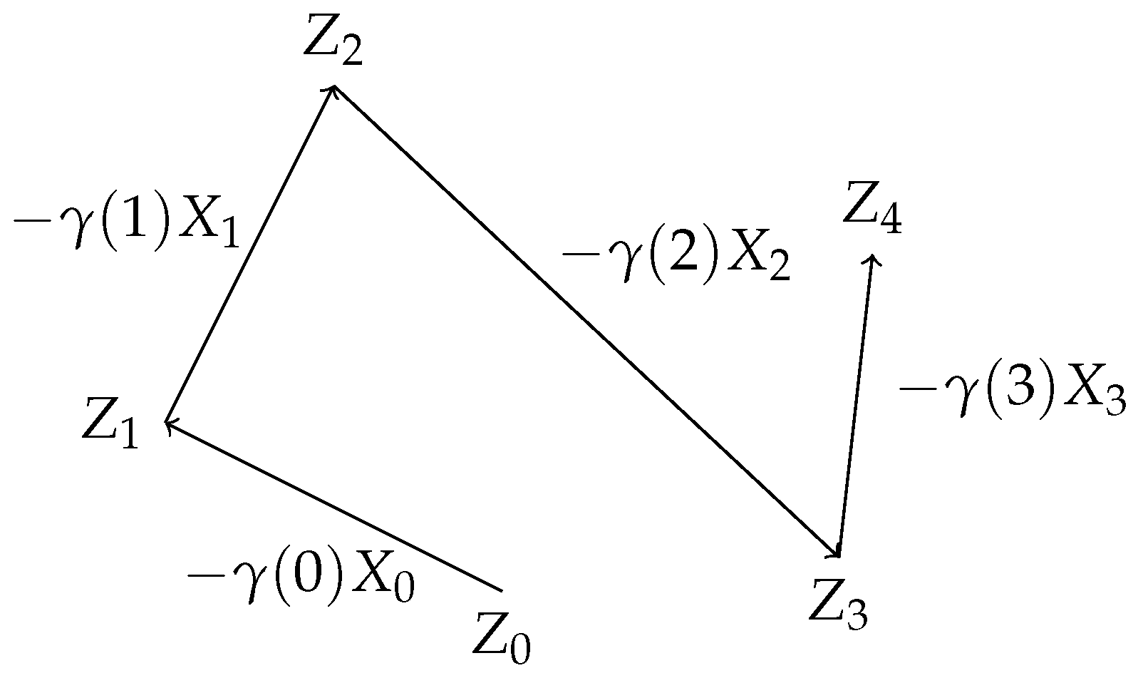
This way of expressing a process allows to define $Z_{t+1}$ with respect to $Z_t$, which gives us control of the difference between both values by means of $\gamma \left(t\right)X\left(t\right)$, as Figure 1 shows. This is very useful if we intend to analyse the convergence of a stochastic process.

Figure 1. Path of stochastic process Z with director process X and learning rate $\gamma$.

As represented in Figure 1, we can think of $Z_t$ as the value of the process at time t, while $-\gamma \left(t\right)X_t$ is the vector going from $Z_t$ to $Z_{t+1}$. For the article, it is important to remember this, since we are constantly referring to $Z_t$ as points in ${\mathbb{R}}^k$ while $X_t$ are managed as direction vectors in ${\mathbb{R}}^k$. This distinction is only practical for our purposes.

The trajectories of stochastic approximation algorithms, such as stochastic gradient descent (SGD), are indeed samples of stochastic processes. Furthermore, they are usually expressed by means of their decomposition of 1-increments, as can be seen in the following examples.

Example 1.

SGD [4] is the cornerstone of machine learning to solve the function optimization problem. The objective of SGD is to minimize an objective function $L\left(\eta \right)={\mathbb{E}}_{z\sim P^{*}}l(\eta ;z)$ for some unknown probability distribution $P^{*}$ and random variable $l\left(\eta \right)$ defined on $({\Omega }^{*},{\mathcal{F}}^{*},P^{*})$. This function l is known as loss function, and it is usually differentiable with respect to η, allowing the definition of SGD as

$$\begin{array}{cc}\hfill Z_{t+1}=& Z_t-\gamma \left(t\right){\nabla }_{\eta }l\left(Z_t\right),\hfill \\ \hfill \gamma \left(t\right)>& 0t\in \mathbb{N}\hfill \end{array}$$

(3)

where $Z_t$ are estimates of $\overline{\eta }$. We can see $Z={\left\{Z_t\right\}}_{t\in \mathbb{N}}$, and, therefore, SGD, as a stochastic process. Indeed, let

$$(\Omega =\prod _{t\in \mathbb{N}}{\Omega }^{*},\mathcal{F}=\prod _{t\in \mathbb{N}}{\mathcal{F}}^{*},P=\prod _{t\in \mathbb{N}}{P}^{*})$$

(4)

be the product probability space (This space is guaranteed to exist according to Kolmogorov extension theorem (see for example Theorem 2.4.4 and following examples in [13])) over infinite sequences. Hence we can define the stochastic process X on $(\Omega ,\mathcal{F},P)$ such that $X_t={\nabla }_{\eta }l\left(Z_t\right)$ where for every $\omega ={\left\{{\omega }_t\right\}}_{t\in \mathbb{N}}\in \Omega$ it is $X_t\left(\omega \right)={\nabla }_{\eta }l(Z_t;{\omega }_t)$. This implies that $(X,\gamma )$ is a decomposition of 1-increments of SGD.

In addition, we observe that $Z_{t+1}$ depends only on last observation $Z_t$ and t, which is known as a non-stationary Markov chain.

Example 2.

This example is worked in [5]. Again, we focus on the function optimization problem, using the same notation as in previous example. In this case, the estimation update of the minimum $\overline{\eta }$ is defined as

$$\begin{array}{cc}\hfill Z_{t+1}=& Z_t-\gamma \left(t\right)B_t·Y_t,\hfill \\ \hfill \gamma \left(t\right)>& 0t\in \mathbb{N}\hfill \end{array}$$

(5)

where $B_t$ is a matrix in ${\mathbb{R}}^{k\times k}$ known after information $Z_0,\cdots ,Z_t$ available at time t and $Y_t=Y\left(Z_t\right)$, where Y is a function mapping each $\eta \in {\mathbb{R}}^k$ to a random variable on the same probability space $({\Omega }^{*},{\mathcal{F}}^{*},P^{*})$.

Similarly as in previous example, Y can be thought as a random variable in the product probability space (Equation (4)) that depends on previous $Z_t$, such that for every $\omega \in \Omega$ it is $Y_t\left(\omega \right)=Y(Z_t;\omega )=Y(Z_t;{\omega }_t)$. If we define $X_t=B_t·Y\left(Z_t\right)$, then $Z=(X,\gamma )$ is a decomposition of 1-increments of Z with $X={\left\{X_t\right\}}_{t\in \mathbb{N}}$.

Here, Z is not a (non-stationary) Markov chain, since $B_t$ may depend on $Z_i$ for all $i<t$.

The naming of $\gamma$ as learning rate is commonly used in the machine learning research branch [4,14,15,16]. The director process X determines the direction $X_t$ at time t of the update Equation (1) with $Z_t$ as reference point, while $\gamma \left(t\right)$ specifies a certain distance to travel along that direction $X_t$. Moreover we demand some constraints to both factors. Condition imposed to $\gamma$ is usually found in the literature [3,4,5]. A learning rate $\gamma$ holds the standard constraint if;

$$\sum _t\gamma {\left(t\right)}^2<\infty ,\sum _t\gamma \left(t\right)=\infty .$$

(6)

Before we show the condition for the director process X, we fix some notation used throughout the article. Consider the natural filtration ${\mathcal{F}}_Z={\left\{{\mathcal{F}}_t\right\}}_{t\in \mathbb{N}}$ generated by stochastic process Z, that is, ${\mathcal{F}}_t=\sigma (Z_i^{-1}\left(A\right)\mid i\le t,A\in \Sigma )$ for all $t\in \mathbb{N}$. Then ${\mathcal{F}}_Z$ is a filtration and by definition Z is adapted to ${\mathcal{F}}_Z$.

Intuitively, every ${\mathcal{F}}_t$ of a filtration is a $\sigma$-algebra that classifies the elements of $\Omega$. For example, if $\Omega$ is the set of colours, ${\mathcal{F}}_t$ can gather warm and cold colours into separate and complementary sets. The fact that a random variable $Z_t$ is ${\mathcal{F}}_t$-measurable implies that $Z_t$ sends all warm colours to the same value and all cold colours also to the same value. Somehow $Z_t$ is then not providing any additional information about elements of $\Omega$ beyond the classification of ${\mathcal{F}}_t$. The sequence ${\mathcal{F}}_t$ is increasing, in the sense that ${\mathcal{F}}_t\subset {\mathcal{F}}_{t+1}$ for all t. Therefore, a filtration characterizes space $\Omega$ with sequentially higher levels of information or classification. Denote ${\mathbb{E}}_t=\mathbb{E}\left[·\mid {\mathcal{F}}_t\right]$ the conditional expectation given ${\mathcal{F}}_t$ [10]. Recall that if Y is a random variable in $(\Omega ,\mathcal{F},P)$ then ${\mathbb{E}}_t\left[Y\right]$ is in turn a ${\mathcal{F}}_t$-measurable random variable.

Hence, if $Z=(X,\gamma )$ then X is locally and linearly bounded by function $\varphi :{\mathbb{R}}^k\to \mathbb{R}$ if

$$(\exists A,B)(\forall t){\mathbb{E}}_t{\parallel X_t\parallel }^2\le A+B·\varphi \left(Z_t\right).$$

(7)

These two constraints are finally combined to present the kind of stochastic processes we are interested in.

Definition 2.

Let Z be a stochastic process and $\varphi :{\mathbb{R}}^k\to \mathbb{R}$ be a function. We say that Z is locally bounded by$\varphi$if there is a decomposition of 1-increments $(X,\gamma )$ with γ holding the standard constraint and X locally and linearly bounded by ϕ.

Furthermore, if $Z_0={\eta }_0$ a.s. we say ${\eta }_0$ is the initial point of Z.

For instance, Examples 1 and 2 observed in this section define Z as a locally bounded process. We see it below.

Example 3.

Recall Example 1. In the same reference [4], the optimization algorithm is asked to hold additional conditions in order to prove its convergence. We added the convergence theorem in Appendix A. Some of the conditions are

$$\begin{array}{c}\hfill \sum _t\gamma {\left(t\right)}^2<\infty ,\sum _t\gamma \left(t\right)=\infty ,\\ \hfill Z_0={\eta }_0\in {\mathbb{R}}^k,\\ \hfill (\exists A,B)(\forall t){\mathbb{E}}_t\parallel X_t{\parallel }^2\le A+B{\parallel Z_t-\overline{\eta }\parallel }^2\end{array}$$

(8)

where $\overline{\eta }\in {\mathbb{R}}^k$ is the optimal point of L. Standard constraint to γ is clearly asked. Moreover ${\eta }_0$ is a starting point. It remains to be seen if X is locally and linearly bounded by some function $\varphi :{\mathbb{R}}^k\to \mathbb{R}$. Indeed, if we define $\varphi \left(\eta \right)=\parallel \eta -\overline{\eta }{\parallel }^2$, then the property is easily checked. Hence Z is locally bounded by ϕ with initial point ${\eta }_0$.

Example 4.

Recall Example 2. Convergence theorem in [5], which is added in the Appendix A, demands below conditions;

$$\begin{array}{c}\hfill \sum _t\gamma {\left(t\right)}^2<\infty ,\sum _t\gamma \left(t\right)=\infty ,\\ \hfill Z_0={\eta }_0\in {\mathbb{R}}^k,\\ \hfill (\exists A,B)(\forall t){\mathbb{E}}_t{\parallel X_t\parallel }^2\le A+BL\left(Z_t\right)\end{array}$$

(9)

where L is a function to optimize. For this example, Z is then locally bounded by $\varphi =L$ with initial point ${\eta }_0$. Just as an observation, property of $B_t$ being determined after information available at time t, is the same as seeing $B_t$ as a ${\mathcal{F}}_t$-measurable random variable over the product probability space.

We are interested on studying the almost sure convergence of Z to a point $\overline{\eta }\in {\mathbb{R}}^k$. A stochastic process Z almost surely (a.s.) converges to a point $\overline{\eta }\in {\mathbb{R}}^k$ if

$$P\left[\omega \in \Omega :\underset{t\to \infty }{lim}{Z}_t\left(\omega \right)=\overline{\eta }\right]=1.$$

(10)

Examples 3 and 4 show us that we can understand the results in [4,5] as the almost sure convergence of some locally bounded processes. In this paper, we are interested in characterizing the almost sure convergence of locally bounded processes. The objective of this work is to create a theory that allows to prove the a.s. convergence of locally bounded processes that covers Examples 3 and 4 and whose applicability generalizes to a wider set of processes, such as the one described below:

Example 5.

Assume the function $f\left(\eta \right)={\parallel \eta \parallel }^2$ defined in ${\mathbb{R}}^k$, and the optimization method Z defined by its director process $X_t=G_1·G_2·Z_t$ where $G_1$ and $G_2$ are positive definite and symmetric matrices. For simplicity, this example shows a stochastic process with no random phenomena associated. We wonder about the convergence of process Z, and if so, whether it converges to the point of ${\mathbb{R}}^k$ that optimizes function f. From Theorems A1 and A2 found in the literature (included in Appendix A) it is not possible to prove a.s. convergence of Z, since conditionsBottou resemblance and C.3, respectively, are not satisfied. That is, because $Z_t{·}^{⊺}{G}_1·G_2·Z_t$ is possibly negative a.s.

Further on, Z is assumed to be locally bounded by $\varphi$ where $(X,\gamma )$ is its corresponding decomposition of 1-increments, unless otherwise indicated.

2.2. Main Result

The objective of the article is to proof below theorem, that we prove in Section 4.1.

Theorem 1.

Let Z be a stochastic process on probability space $(\Omega ,\mathcal{F},P)$. Then Z almost surely converges to a point $\overline{\eta }$ if there is a twice differentiable convex function ϕ with unique minimum $\overline{\eta }$ defined in ${\mathbb{R}}^k$ with bounded Hessian norm, such that

• Z is locally bounded by ϕ;
• Z resembles $\nabla \varphi$.

There is one concept of the theorem that needs a definition. That is, when a stochastic process resembles to a vector field. Next sections have that end, with our main definition that fills the gap appearing at Section 3.2. As we will see in Section 4.4, simple Example 5 finds a solution with our main theorem.

2.3. Expected Direction Set

We now define one key object of our work named the expected direction set. It focuses on gathering all directions that the update may take at time t conditioned to ${\mathcal{F}}_t$. Before the definition we provide some concepts and notation.

Random variable ${\mathbb{E}}_t\left[X_t\right]$ determines all expected directions of Z at time t that the stochastic process may follow assuming ${\mathcal{F}}_t$. For example, if $\omega \in \Omega$ is an observation, then ${\mathbb{E}}_t\left[X_t\right]\left(\omega \right)\in {\mathbb{R}}^k$ is a vector pointing to the expected update direction departing from point $Z_t\left(\omega \right)$ given ${\mathcal{F}}_t$. Denote the expected direction of Z at $\omega \in \Omega$ and time t as

$$D_Z(\omega ,t)={\mathbb{E}}_t\left[X_t\right]\left(\omega \right).$$

(11)

The expected direction from point $\eta =Z_t\left(\omega \right)$ of Equation (11) depends on $\omega$. That is, the path followed until reaching $\eta =Z_t\left(\omega \right)\in {\mathbb{R}}^k$ matters. For instance, if ${\omega }_1,{\omega }_2\in \Omega$ are different observations, such that $\eta =Z_t\left({\omega }_1\right)=Z_t\left({\omega }_2\right)$, then possibly $D_Z({\omega }_1,t)\ne D_Z({\omega }_2,t)$. We collect all expected directions at $\eta =Z_t\left(\omega \right)$ and time t in the vector set below;

$$S_Z(\eta ,t)=\{D_Z(\omega ,t)\mid \omega \in \Omega ,Z_t\left(\omega \right)=\eta \}.$$

(12)

The tools to define the expected direction set at $\eta \in {\mathbb{R}}^k$ after time $T\in \mathbb{N}$ are given, so we proceed to its formal definition.

Definition 3.

Let $Z=(X,\gamma )$. Define the expected directions set of Z at $\eta \in {\mathbb{R}}^k$ after time $T\in \mathbb{N}$ as

$$ED{S}_Z(\eta ,T):=\bigcup _{t\ge T}{S}_Z(\eta ,t).$$

(13)

With a few words, $ED{S}_Z(\eta ,T)$ is a vector set containing all expected directions (provided by the director process X) conditioned to ${\mathcal{F}}_t$ for every outcome $\omega$ such that $Z_t\left(\omega \right)=\eta$ where $t\ge T$. In Definition 3, $EDS$ depends on T. That is because to assess the convergence of an algorithm it is not important to consider all expected directions throughout all the process. For example, if an algorithm converges we can modify randomly all directions of the director process for just a particular time $T\in \mathbb{N}$, and the resulting algorithm still converges. Roughly speaking, only the tail of a process matters to determine the convergence property. This concept is better addressed with Definition 4 in next section.

Example 6.

Recall Example 1. Assume that Z is then SGD. Then $ED{S}_Z(\eta ,T)$ is a singleton. Indeed, $D_Z(\omega ,t)$ is the same vector for all $t\in \mathbb{N}$ and all ω with $Z_t\left(\omega \right)=\eta$ and hence $S_Z(\eta ,t)=\left\{D_Z(\omega ,t)\right\}$ with any $\omega \in \Omega$ with $Z_t\left(\omega \right)=\eta$. Finally

$$ED{S}_Z(\eta ,T)=\left\{{\mathbb{E}}_t\left[X_t\right]\left(\omega \right)\right\}forany\omega \in \Omega andt\ge Twith{Z}_t\left(\omega \right)=\eta .$$

(14)

This is the case of any non-stationary Markov chain.

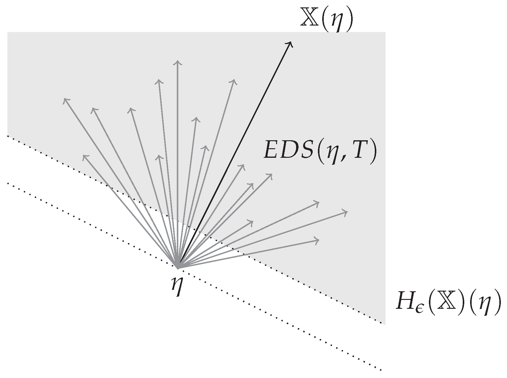
2.4. Essential Expected Direction Set

Convergence property of an algorithm relates closely to directions followed after time $T\in \mathbb{N}$ as T tends to infinity. Equivalently, the direction set appearing repeatedly through the whole optimization process matters, while directions set only contemplated for a finite amount of iterations changes nothing, in terms of convergence guarantee. This direction set is named the essential expected directions set in this article.

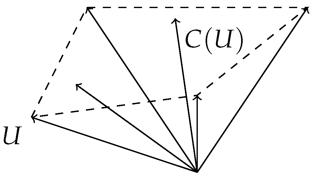
To define properly the essential expected directions set, we will use the convex vector subspace of a given vector set. Given a vector set U in ${\mathbb{R}}^k$, let $C\left(U\right)$ be the smallest convex vector subspace containing U. See Figure 2 as an illustrative example. Observe that $C\left(U\right)$ is always closed, but it may be unbounded.

Figure 2. Set of vectors U and its convex vector subspace $C\left(U\right)$ in ${\mathbb{R}}^2$.

Definition 4.

Let $Z=(X,\gamma )$. Define the essential expected directions set of Z at η as

$$EED{S}_Z\left(\eta \right):={\cap }_{T}C\left(ED{S}_Z(\eta ,T)\right).$$

(15)

Example 7.

Assume Z is any non-stationary Markov chain, such that SGD in Example 1. Then $EED{S}_Z\left(\eta \right)=ED{S}_Z(\eta ,T)$ for any T. Indeed, we have seen in Example 6 that $ED{S}_Z(\eta ,T)=\left\{{\mathbb{E}}_t\left[X_t\right]\left(\omega \right)\right\}$ for any $\omega \in \Omega$ and $t\ge T$ where $Z_t\left(\omega \right)=\eta$. Hence

$$EED{S}_Z\left(\eta \right)={\cap }_{T}C\left(ED{S}_Z(\eta ,T)\right)=C\left(\left\{{\mathbb{E}}_t\left[X_t\right]\left(\omega \right)\right\}\right)=\left\{{\mathbb{E}}_t\left[X_t\right]\left(\omega \right)\right\}=ED{S}_Z(\eta ,T),$$

(16)

for any $\omega \in \Omega$ with $Z_T\left(\omega \right)=\eta$.

Definition of $EED{S}_Z\left(\eta \right)$ delimits the smallest subspace where all directions at $\eta$ tend to. Clearly, $EED{S}_Z\left(\eta \right)$ is also convex and closed (possibly empty). Deeper properties of this set lead to identify divergence symptoms. For example, if it is empty or unbounded, we face instability of the process at $\eta$. To see this, observe below result. The proof can be found in the Appendix B.

Corollary 1.

Let $\eta \in {\mathbb{R}}^k$. Then $EED{S}_Z\left(\eta \right)$ is a non-empty bounded set if, and only if, there exists $T\in \mathbb{N}$, such that $C\left(ED{S}_Z(\eta ,T)\right)$ is bounded.

This result relates $EED{S}_Z\left(\eta \right)$ with instability properties of Z. If $EED{S}_Z\left(\eta \right)$ is empty or unbounded, then the algorithm is unstable at $\eta$, since expected directions with arbitrarily large norms exist after enough iterations. Clearly, if this situation is found for all points near the optimum, the algorithm can not converge to the solution. It is desirable instead that $C\left(ED{S}_Z(\eta ,T)\right)$ is compact (bounded) for some T for every $\eta \in {\mathbb{R}}^k$, or equivalently, that $EED{S}_Z\left(\eta \right)$ is compact (bounded) and not empty.

In fact, since we are interested in the case where Z is locally bounded by $\varphi$ (recall Definition 2), we can assume that $EED{S}_Z\left(\eta \right)$ is a non empty compact set, by virtue of below results.

Proposition 1.

Let stochastic process Z be locally bounded by ϕ. Then $C\left(ED{S}_Z(\eta ,0)\right)$ is a non-empty compact set.

Proof. 

We know that X is locally and linearly bounded. Hence, applying Jensen’s inequality

$$\parallel {\mathbb{E}}_t\left[X_t\right]{\parallel }^2\le {\mathbb{E}}_t{\parallel X_t\parallel }^2\le A+B·\varphi \left(Z_t\right).$$

(17)

Let $\eta \in {\mathbb{R}}^k$ and $\omega \in \Omega$, such that $Z_t\left(\omega \right)=\eta$ for some $t\ge 0$. Therefore, every $v={\mathbb{E}}_t\left[X_t\right]\left(w\right)\in ED{S}_Z(\eta ,0)$ has bounded norm by $A+B·\varphi \left(\eta \right)$, implying that $C\left(ED{S}_Z(\eta ,0)\right)$ is a non-empty compact set. □

Below corollary is a consequence of Proposition 1 and Corollary 1.

Corollary 2.

Let stochastic process Z be locally bounded by ϕ. Then $EED{S}_Z\left(\eta \right)$ is a non-empty compact set for all $\eta \in {\mathbb{R}}^k$.

3. Vector Field Half-Spaces and Stochastic Processes. Resemblance

This section defines the main concept of this work; the property of resemblance between a stochastic process and a vector field. The definition highlight some commonalities between Theorems A1 and A3. Both of them prove the convergence of stochastic processes that resemble to particular vector fields. A geometric interpretation and explanation of convergence theorems conditions is established in next Section 4.

Some previous definitions are needed and stated before introducing the main concepts of the article, such as $ϵ$-acute vector pair sets and the half-space of a vector field. The section starts with some basic concepts about vectors.

Definition 5.

Let $u,v\in {\mathbb{R}}^k$ be two vectors. The pair $(u,v)$ is acute if u and v form an acute angle, that is, if $u^{⊺}·v>0$. Furthermore, if $u^{⊺}·v\ge ϵ>0$ then $(u,v)$ is ϵ-acute.

Proposition 2.

Let $u,v\in {\mathbb{R}}^k$ be two vectors. Then the pair $(u,v)$ is ϵ-acute if, and only if, there exists a symmetric positive-definite matrix B, such that $B·u=v$ and $u^{⊺}·B·u\ge ϵ$.

A vector pair set V is a set of vector pairs $V=\{(u_i,v_i)\in {\left({\mathbb{R}}^k\right)}^2\mid i\in I\}$ where I is an index set.

Definition 6.

Let V be a vector pair set. V is ϵ-acute if every vector pair $(u,v)\in V$ is ϵ-acute.

Next result is a direct consequence.

Proposition 3.

Let V be a vector pair set, indexed by I. Then, V is ϵ-acute for some $ϵ>0$ if, and only if;

$$\underset{\begin{array}{c}i\in I\\ (u_i,v_i)\in V\end{array}}{inf}{u}_i^{⊺}{v}_i>0.$$

(18)

Proposition 4.

Let V be a vector pair set, indexed by I. Then, V is ϵ-acute for some $ϵ>0$ if, and only if, there exist a set of symmetric positive-definite matrices $B=\{B_i\mid i\in I\}$ such that

$$\begin{array}{cc}\hfill \underset{\begin{array}{c}i\in I\\ (u_i,v_i)\in V\end{array}}{inf}{u}_i^{⊺}{B}_i{u}_i& >0,\hfill \\ \hfill B_i{u}_i& =v_i.\hfill \end{array}$$

(19)

Proof. 

Prove, first, that if there exist a set of matrices $B=\{B_i\mid i\in I\}$ holding Equation (19) then V is $ϵ$-acute for some $ϵ>0$. Observe that after Equation (19);

$$\underset{i\in I}{inf}{u}_i^{⊺}{v}_i=\underset{i\in I}{inf}{u}_i^{⊺}{B}_i{u}_i>0.$$

(20)

Then, Proposition 3 implies that V is $ϵ$-acute and finishes this part of the proof.

Now assume that V is $ϵ$-acute, prove then that there exist a set of matrices $B=\{B_i\mid i\in I\}$ holding Equation (19). Since V is $ϵ$-acute, in particular, the pair $(u_i,v_i)\in V$ is $ϵ$-acute for every $i\in I$. Apply Proposition 2: for every $i\in I$ there exists a symmetric positive-definite matrix $B_i$, such that $B_i{u}_i=v_i$ and $u_i^{⊺}·B_i·u_i\ge ϵ$. This finishes the proof. □

3.1. The Half-Space of a Vector Field

The half-space determined by a vector u is the set of vectors that conform an acute angle with u. This region clearly occupies half of the total space. Additionally, the $ϵ$-half-space of u with $ϵ>0$ is the set of vectors v, such that the vector pair $(u,v)$ is $ϵ$-acute. This object is needed for afterwards defining the half-space of a vector field. We define these concepts below and illustrate the $ϵ$-half-space of a vector u in Figure 3.

Figure 3. Shaded area representing $H_{ϵ}\left(u\right)$.

Definition 7.

Let u be a vector of ${\mathbb{R}}^k$. The half-space of u is the set

$$H\left(u\right)=\{v\in {\mathbb{R}}^k\mid u^{⊺}·v>0\}.$$

(21)

Similarly, the ϵ-half-space of u with $ϵ>0$ is the set

$$H_{ϵ}\left(u\right)=\{v\in {\mathbb{R}}^k\mid u^{⊺}·v\ge ϵ\}.$$

(22)

A vector field $\mathbb{X}$ over ${\mathbb{R}}^k$ is a function assigning to every $\eta \in {\mathbb{R}}^k$ a vector of ${\mathbb{R}}^k$, that is $\mathbb{X}:{\mathbb{R}}^k\to {\mathbb{R}}^k$. For example, if $l:{\mathbb{R}}^k\to \mathbb{R}$ is a twice differentiable function, we can consider the vector field consisting of the gradient vectors at each point $\eta$. Precisely, denote the gradient vector field (GVF) as ${\mathbb{X}}_{\nabla l}$, where ${\mathbb{X}}_{\nabla l}\left(\eta \right)=\nabla l\left(\eta \right)$.

We are ready to define the half-space of a vector field.

Definition 8.

Let $\mathbb{X}$ be a vector field over ${\mathbb{R}}^k$. The half-space of $\mathbb{X}$ is a function $H\left(\mathbb{X}\right)$ mapping every η to $H\left(\mathbb{X}\right)\left(\eta \right)=H\left(\mathbb{X}\left(\eta \right)\right)$. Similarly, the ϵ-half-space of $\mathbb{X}$ with $ϵ>0$ is a function $H_{ϵ}\left(\mathbb{X}\right)$ mapping every η to $H_{ϵ}\left(\mathbb{X}\right)\left(\eta \right)=H_{ϵ}\left(\mathbb{X}\left(\eta \right)\right)$.

3.2. Resemblance between a Stochastic Process and a Vector Field

The convergence of any locally bounded process can be proved comparing the expected directions set of the algorithm with some vector fields. When the expected directions resemble the vector field we compare it to, then we can ensure the almost sure convergence to a point of the stochastic process, after some reasonable conditions. By resemblance, we mean that the expected directions set after some time T is a subset of the $ϵ$-half-space of $\mathbb{X}$, among other things explained later. Therefore, resemblance asks for every $\eta \in {\mathbb{R}}^k$ that every vector $D_Z(\omega ,t)$ with $t\ge T$ and every $\omega \in \Omega$ with $\eta =Z_t\left(\omega \right)$ form an acute angle with the vector field at $\mathbb{X}\left(\eta \right)$.

However, if the vector field sends a specific point $\eta$ to $0\in {\mathbb{R}}^k$, then no direction can be set by the $D_Z(\omega ,t)$ to form an acute vector pair. Therefore, resemblance property is evaluated outside the neighborhood of these annulled points. That is why we must consider now the set of annulled points of a vector field and the neighborhoods around the points of this set.

Formally, let $\mathbb{X}$ be a vector field defined in ${\mathbb{R}}^k$. The set $K_{\mathbb{X}}$ is the set of points of ${\mathbb{R}}^k$ annulled by $\mathbb{X}$, that is, $K_{\mathbb{X}}:=\{\eta \in {\mathbb{R}}^k\mid \mathbb{X}\left(\eta \right)=0\}$. Moreover, consider the closed ball centered on $K_{\mathbb{X}}$ of radius $\delta$ as $B_{\delta }\left(K_{\mathbb{X}}\right):={\cup }_{\eta \in K_{\mathbb{X}}}{B}_{\delta }\left(\eta \right)$ where $B_{\delta }\left(\eta \right)$ is the closed ball of radius $\delta$ centered on $\eta$.

We also use the notation $A^{\prime }={\mathbb{R}}^k\setminus A$ for the compliment set of subset $A\subset {\mathbb{R}}^k$. We say that Zϵ-resembles to $\mathbb{X}$ at $\eta$ from T on if $ED{S}_Z(\eta ,T)\subset H_{ϵ}\left(\mathbb{X}\right)\left(\eta \right)$. Observe an illustrative example in Figure 4.

Figure 4. A stochastic process Z that $ϵ$-resembles to $\mathbb{X}$ at $\eta$ from T on, since vector set $ED{S}_Z(\eta ,T)$ of all expected directions of Z at $\eta$ after time T belongs to $H_{ϵ}\left(\mathbb{X}\right)\left(\eta \right)$.

This intuition is naturally extended to ϵ-resemblance at sets, when the property is satisfied for every $\eta$ in the set. With this in mind we can define the key concept of this article.

Definition 9.

Let $Z=(X,\gamma )$ be a stochastic process and $\mathbb{X}$ be a vector field over ${\mathbb{R}}^k$. We say that Z resembles to $\mathbb{X}$ from $T\in \mathbb{N}$ on, if;

$$(\forall \delta >0)(\exists ϵ>0)Zϵ-\mathrm{resembles}\mathrm{to}\mathbb{X}\mathrm{at}{B}_{\delta }{\left(K_{\mathbb{X}}\right)}^{\prime }\mathrm{from}T\mathrm{on}$$

(23)

We say that Z resembles to $\mathbb{X}$ if there is $T\in \mathbb{N}$ such that it resembles to $\mathbb{X}$ from T on.

Everything is set up to accomplish the goal of this paper. We refresh the main theorem of this article in next section and show its proof.

4. Proof of Main Result. Reinterpretation of Convergence Theorems

The objective of the article is within reach now. That is, proving main Theorem 1. Moreover, this section addresses afterwards the task of proving that Theorems A1 and A3 are particular examples of our main Theorem 1.

4.1. Resemblance to Conservative Vector Fields and Convergence

Recall main Theorem 1 and observe that it asks the stochastic process Z to be locally bounded by some function $\varphi$ and Z to resemble to $\nabla \varphi$. Therefore, $\nabla \varphi$ is a particular type of vector field called conservative vector field. That is, a vector field that appears from derivation of a function. That is why we understand our main theorem as a convergence result of locally bounded processes of resemblance to conservative vector field.

In the theorem statement, it says that $\varphi$ has bounded Hessian norm. Similarly to Theorem A3, it means that:

$$(\exists K)(\forall \eta )\parallel {\nabla }_{\eta }^2\varphi \left(\eta \right)\parallel \le K^{\prime }.$$

We are ready to prove the main result of the paper.

Proof of main Theorem 1.

Observe that $\varphi$ is bounded from below. Indeed, $\overline{\eta }$ is a minimum and $\varphi$ is convex with $\mathbb{X}\left(\overline{\eta }\right)=0$ where $\mathbb{X}=\nabla \varphi$. Therefore, there exists a constant $m\ge 0$ such that $\varphi \left(\eta \right)+m\ge 0$ for all $\eta$. Define $\psi \left(\eta \right)=\varphi \left(\eta \right)+m$. Clearly, $\nabla \psi =\nabla \varphi =\mathbb{X}$, and, therefore, Zresembles to $\nabla \psi$. Moreover, Z is locally bounded by $\psi$ and $\psi$ clearly satisfies the Hessian norm bound.

From here, the prove follows the steps of Theorem A2’s proof. Taylor inequality and Hessian norm bound;

$$\begin{array}{cc}\hfill \psi \left(Z_{t+1}\right)& =\psi (Z_t-{\gamma }_t{X}_t)\hfill \\ \hfill & \le \psi \left(Z_t\right)-{\gamma }_t\mathbb{X}{\left(Z_t\right)}^{⊺}{X}_t+{\gamma }_t^{2}K{\parallel X_t\parallel }^2\hfill \end{array}$$

(24)

where $K=\frac{K^{\prime }}{2}$. Apply expectation conditioned to information until time t and then use that Z is locally bounded by $\psi$;

$$\begin{array}{cc}\hfill {\mathbb{E}}_t\psi \left(Z_{t+1}\right)& \le \psi \left(Z_t\right)-{\gamma }_t\mathbb{X}{\left(Z_t\right)}^{⊺}{\mathbb{E}}_t\left[X_t\right]+{\gamma }_t^{2}K{E}_t\left[\parallel X_t{\parallel }^2\right]\hfill \\ \hfill & \le \psi \left(Z_t\right)-{\gamma }_t\mathbb{X}{\left(Z_t\right)}^{⊺}{\mathbb{E}}_t\left[X_t\right]+{\gamma }_t^{2}K(A+B\psi \left(Z_t\right))\hfill \\ \hfill & \le (1+{\gamma }_t^{2}KB)\psi \left(Z_t\right)-{\gamma }_t\mathbb{X}{\left(Z_t\right)}^{⊺}{\mathbb{E}}_t\left[X_t\right]+{\gamma }_t^{2}KA.\hfill \end{array}$$

(25)

Use now that Zresembles to $\mathbb{X}$. Then, there exists T such that for every $t\ge T$, the term $-{\gamma }_t\mathbb{X}{\left(Z_t\right)}^{⊺}{\mathbb{E}}_t\left[X_t\right]$ is negative. All other conditions of Robbins–Siegmund theorem (in [7], added in Appendix A) also hold for the algorithm after time T, thanks to learning rate constraints. Apply it and deduce that random variables $\psi \left(Z_t\right)$ converge almost surely to a random variable (and so does $\varphi \left(Z_t\right)$) and that;

$$\sum _t{\gamma }_t\mathbb{X}{\left(Z_t\right)}^{⊺}{\mathbb{E}}_t\left[X_t\right]<\infty \mathrm{a}.\mathrm{s}.$$

(26)

Prove now that stochastic process $\varphi \left(Z_t\right)$ converges almost surely to value $\varphi \left(\overline{\eta }\right)$. Proceed by contradiction. Assume that for ${\delta }_1>0$

$$P\left[\omega \in \Omega \mid \underset{t}{lim}\varphi \left(Z_t\left(w\right)\right)\in B_{{\delta }_1}{\left(\varphi \left(\overline{\eta }\right)\right)}^{\prime }\right]>0$$

(27)

this implies, by continuity and convexity of function $\varphi$, that there exists $\delta$

$$P\left[A=\{\omega \in \Omega \mid \underset{t}{lim}{Z}_t\left(w\right)\in B_{\delta }{\left(\overline{\eta }\right)}^{\prime }\}\right]>0.$$

(28)

By resemblance and definition of the limit, there exists T and $ϵ$ such that $ED{S}_Z(\eta ,T)\subset H_{ϵ}\left(\mathbb{X}\right)\left(\eta \right)$ for every $\eta \in B_{\delta }{\left(\overline{\eta }\right)}^{\prime }$. This leads to a contradiction, since using learning rate standard constraint we have

$$\sum _{t\ge T}{\gamma }_t\mathbb{X}{\left(Z_t\left(\omega \right)\right)}^{⊺}{\mathbb{E}}_t\left[X_t\right]\left(\omega \right)>\sum _{t\ge T}{\gamma }_t·ϵ=\infty$$

(29)

for every $\omega \in A$, which has measure different to 0 by Equation (28). This clearly contradicts Equation (26).

Hence, $\varphi \left(Z_t\right)$ converges almost surely to $\varphi \left(\overline{\eta }\right)$ and $Z_t$ converges almost surely to $\overline{\eta }$ as wanted. □

4.2. Reinterpretation of Bottou’s Convergence Theorem

The goal now is to deduce Theorem A1 as a direct consequence of main Theorem 1. Consider a particular case of main Theorem 1 where $\varphi \left(\eta \right)=\parallel \eta -\overline{\eta }{\parallel }^2$, that reads as follows.

Corollary 3.

Let $\varphi \left(\eta \right)=\parallel \eta -\overline{\eta }{\parallel }^2$ and Z be a stochastic process on probability space $(\Omega ,\mathcal{F},P)$. Then Z almost surely converges to $\overline{\eta }$ if

• Z is locally bounded by ϕ;
• Z resembles $\nabla \varphi$.

Additional conditions to $\varphi$, such as Hessian bound or twice differentiability, are not specified in the corollary since with the particular definition of $\varphi$ all those conditions are already satisfied.

To see that Corollary 3 proves Theorem A1 statement, we need to prove that Theorem A1 is assuming that Z is locally bounded by $\varphi$ and that Z resembles $\nabla \varphi$. Example 3 already proves that Bottou is assuming that Z is locally bounded by $\varphi$. Therefore, it remains to check that Z resembles to $\nabla \varphi$. To that end, see below proposition proved in Appendix C.

Proposition 5.

Let $Z=(X,\gamma )$ be a stochastic process and $\mathbb{X}$ be a vector field over ${\mathbb{R}}^k$. Then Z resembles to $\mathbb{X}$ if, and only if,

$$(\exists T\in \mathbb{N})(\forall \delta >0)\underset{\begin{array}{c}\eta \in {\mathbb{R}}^k\setminus B_{\delta }\left(K_{\mathbb{X}}\right)\\ v\in ED{S}_Z(\eta ,T)\end{array}}{inf}\mathbb{X}{\left(\eta \right)}^{⊺}·v>0.$$

(30)

Observe condition Bottou resemblance of Theorem A1 and Proposition 5. Deduce from it, that the algorithm Z of the theorem resembles to vector field $\nabla \varphi$.

Corollary 4.

Let $Z=(X,\gamma )$ be a stochastic process and $\overline{\eta }\in {\mathbb{R}}^k$. Then Z resembles to $\nabla \varphi$ with $\varphi \left(\eta \right)=\parallel \eta -\overline{\eta }{\parallel }^2$ if, and only if,Bottou resemblanceholds.

4.3. Reinterpretation of Sunehag’s Convergence Theorem

Theorem A3 is deduced from main Theorem 1. Similarly to previous section, we provide a version of our main theorem for the case where $\varphi =l$ is a function that we aim to minimize.

Corollary 5.

Let $l:{\mathbb{R}}^k\to \mathbb{R}$ be a twice differentiable cost function with a unique minimum $\overline{\eta }$ and bounded Hessian norm, and let Z be a stochastic process on probability space $(\Omega ,\mathcal{F},P)$. Then Z converges to the minimum $\overline{\eta }$ of l almost surely if

• Z is locally bounded by l;
• Z resembles $\nabla l$.

The stochastic process described in Theorem A3 has some more properties, such as $X_t=B_t·Y_t$. However, if we prove that Z of that theorem is locally bounded by l and that Zresembles$\nabla l$, then it is clear that Corollary 5 deduces Theorem A3. Recall Example 4 and notice that we already proved that Z is locally bounded by l. The remaining property is acquired after below proposition that we prove in Appendix D.

Proposition 6.

Let $Z=(X,\gamma )$ be a stochastic process and $\mathbb{X}$ be a vector field over ${\mathbb{R}}^k$. Then Z resembles to $\mathbb{X}$ if, and only if, there exists T, such that for every $t\ge T$ there are random vectors $Y_t$ to ${\mathbb{R}}^k$ and symmetric and positive-definite ${\mathcal{F}}_t$-measurable random matrices $B_t$ such that

$$B_t·Y_t=X_t,$$

(31)

$${\mathbb{E}}_t\left[Y_t\right]=\mathbb{X}\left(Z_t\right)Z_t\left(\omega \right)\notin K_{\mathbb{X}},$$

(32)

$$(\forall \delta >0)\underset{\begin{array}{c}\eta \in {\mathbb{R}}^k\setminus B_{\delta }\left(K_{\mathbb{X}}\right)\\ t\ge T\\ \omega \in \Omega ,Z_t\left(\omega \right)=\eta \end{array}}{inf}\mathbb{X}{\left(\eta \right)}^{⊺}·B_t\left(\omega \right)·\mathbb{X}\left(\eta \right)>0.$$

(33)

It is only necessary to put together Proposition 6 and condition C.1 and Sunehag resemblance to finish our objective with the following corollary

Corollary 6.

Let l be a differentiable function and $Z=(X,\gamma )$ be a stochastic process. Then Z resembles to $\nabla l$ if, and only if, there exist T such that for every $t\ge T$ there are random vectors $Y_t$ to ${\mathbb{R}}^k$ and symmetric and positive-definite ${\mathcal{F}}_t$-measurable random matrices $B_t$ such that $B_t·Y_t=X_t$ and conditionsC.1andSunehag resemblancehold.

Corollaries 4 and 6 nicely show the value of Theorem 1 for proving convergence. To reinforce this, we notice that the convergence of algorithm DSNGD in [12] is easily proved by means of Corollary 5, by combining both Theorem A3 and Corollary 6. This shows that Theorem 1 allows to prove convergence of a wider set of stochastic processes and function optimization methods.

4.4. Convergence of Process in Example 5

Our theorem solves question proposed by Example 5. To see it, just define

$$\varphi \left(\eta \right)=\frac{1}{2}{\eta }^{⊺}·G_2·\eta .$$

(34)

Twice differentiable and convex function $\varphi$ has bounded Hessian norm, since its Hessian is the constant matrix $G_2$. Moreover, Z is clearly locally bounded by $\varphi$. Indeed, recall Equation (7) and observe;

$$\parallel G_1·G_2·Z_t{\parallel }^2\le B·\varphi \left(Z_t\right)$$

(35)

where $B=\frac{2{\lambda }_1^2·{\lambda }_2^2}{{\mu }_2}$ such that ${\lambda }_i$ is the greatest eigenvalue of $G_i$ and ${\mu }_i$ is the least eigenvalue of $G_i$.

Finally, check that Zresembles to $\nabla \varphi \left(\eta \right)=G_2\eta$. Observe that $ED{S}_Z(\eta ,T)=\left\{G_1{G}_2\eta \right\}$ is a singleton for every T. Then for all $\delta >0$ and all $\eta \in B_{\delta }\left(K_{\nabla \varphi }\right)$ it is

$$\nabla \varphi {\left(\eta \right)}^{⊺}·G_1{G}_2\eta ={\eta }^{⊺}{G}_2·G_1{G}_2\eta \ge ϵ,$$

(36)

where $ϵ={\mu }_1·{\mu }_2^2·{\delta }^2$. Hence Z resembles to $\nabla \varphi$ and by virtue of our main Theorem 1 process Z converges a.s. to 0, and, therefore, minimizes function f as wanted.

5. Conclusions

We have presented a result that allows us to prove the convergence of stochastic processes. We have proven that two useful convergence results in the literature are a consequence of our theorem. This is made after a new theory that compares the expected directions of the algorithm to conservative vector fields. If the expected directions at a point $\eta$ resemble enough to vector $\mathbb{X}\left(\eta \right)$ with $\nabla \varphi =\mathbb{X}$ a conservative vector field, then the process is stable at that point. If this happens for every $\eta \in {\mathbb{R}}^k$, and in addition the process is locally bounded by $\varphi$, then the process is globally stable and converges.

Some inspiring paths remain unexplored after this work. For example, finding $\varphi$ function is the key to prove convergence, and it is asked to be a convex twice differentiable function. It is interesting to study how function $\varphi$ can be obtained, for instance as a sum of other convex twice differentiable functions ${\varphi }_i$.

Another promising research line is a deeper analysis of $EDS$ and $EEDS$ objects, which may guarantee the existence of a function $\varphi$ without the need of finding it. If sufficient conditions are established for a stochastic process to ensure resemblance to some unknown conservative vector field, then $\varphi$ searching can be dodged. Even proving the non-existence of such function after a wider study of $EDS$ and $EEDS$ is useful, forbidding the use of our theorem.

It is also interesting to study the converse implication. Specifically, investigating the conditions that lead to divergent instances after ground theory explained in the article. In this sense, Lyapunov characterization of convergent processes becomes a helpful and key theory, since great similarities arise between these two techniques.

Furthermore, in many occasions the function $\varphi$ to optimize can be established beforehand (convex and twice differentiable). Therefore, the opposite process can be considered, that is, generating a set of stochastic processes that resemble to $\nabla \varphi$, assuring in consequence the convergence of such candidates.

In [17], one finds another relevant convergence result. It assures the convergence in probability of a stochastic process, instead of almost sure convergence worked in this article. We wonder about the existing commonalities with our theorem, and the possibility to relax the conditions our theorem imposes, yet ensuring convergence in probability of a process.

We are currently working on two weaker resemblance properties, that we name weak and essential resemblance. The intention is to deduce almost sure convergence of a process by only studying its essential expected direction set (EEDS).

References

- Amari, S.I. Natural Gradient Works Efficiently in Learning. Neural Comput. 1998, 276, 251–276. [Google Scholar] [CrossRef]
- Thomas, P.S. GeNGA: A generalization of natural gradient ascent with positive and negative convergence results. In Proceedings of the 31st International Conference on Machine Learning, ICML 2014, Beijing, China, 21–26 June 2014; Volume 5, pp. 3533–3541. [Google Scholar]
- Sánchez-López, B.; Cerquides, J. Convergent Stochastic Almost Natural Gradient Descent. In Proceedings of the Artificial Intelligence Research and Development-Proceedings of the 22nd International Conference of the Catalan Association for Artificial Intelligence, Mallorca, Spain, 23–25 October 2019; Volume 319, pp. 54–63. [Google Scholar]
- Bottou, L. Online Algorithms and Stochastic Approximations. In Online Learning and Neural Networks; Saad, D., Ed.; Cambridge University Press: Cambridge, UK, 1998; Revised, October 2012. [Google Scholar]
- Sunehag, P.; Trumpf, J.; Vishwanathan, S.V.N.; Schraudolph, N. Variable Metric Stochastic Approximation Theory. In Proceedings of the Artificial Intelligence and Statistics, Clearwater, FL, USA, 16–19 April 2009; pp. 560–566. [Google Scholar]
- Lyapunov, A.M. The general problem of the stability of motion. Int. J. Control 1992, 55, 531–534. [Google Scholar] [CrossRef]
- Robbins, H.; Siegmund, D. A convergence theorem for non negative almost supermartingales and some applications. In Optimizing Methods in Statistics; Rustagi, J.S., Ed.; Academic Press: Cambridge, MA, USA, 1971; pp. 233–257. [Google Scholar]
- Karlin, S.; Taylor, H.M. Elements of stochastic processes. In A First Course in Stochastic Processes, 2nd ed.; Karlin, S., Taylor, H.M., Eds.; Academic Press: Boston, MA, USA, 1975; Chapter 1; pp. 1–44. [Google Scholar] [CrossRef]
- Ross, S.M.; Kelly, J.J.; Sullivan, R.J.; Perry, W.J.; Mercer, D.; Davis, R.M.; Washburn, T.D.; Sager, E.V.; Boyce, J.B.; Bristow, V.L. Stochastic Processes; Wiley: New York, NY, USA, 1996; Volume 2. [Google Scholar]
- Bass, R.F. Stochastic Processes; Cambridge University Press: Cambridge, UK, 2011; Volume 33. [Google Scholar]
- Grimmett, G.; Stirzaker, D. Probability and Random Processes; OUP Oxford: Oxford, UK, 2020. [Google Scholar]
- Sánchez-López, B.; Cerquides, J. Dual Stochastic Natural Gradient Descent and convergence of interior half-space gradient approximations. arXiv 2021, arXiv:2001.06744. [Google Scholar]
- Tao, T. An Introduction to Measure Theory; Graduate Studies in Mathematics, American Mathematical Society: Providence, RI, USA, 2011. [Google Scholar]
- Duchi, J.; Hazan, E.; Singer, Y. Adaptive Subgradient Methods for Online Learning and Stochastic Optimization. J. Mach. Learn. Res. 2011, 12, 2121–2159. [Google Scholar]
- Zeiler, M.D. ADADELTA: An Adaptive Learning Rate Method. arXiv 2012, arXiv:1212.5701. [Google Scholar]
- Kingma, D.P.; Ba, L.J. Adam: A Method for Stochastic Optimization. In Proceedings of the 3rd International Conference on Learning Representations (ICLR), San Diego, CA, USA, 7–9 May 2015. [Google Scholar]
- Robbins, H.; Monro, S. A Stochastic Approximation Method. Ann. Math. Stat. 1951, 22, 400–407. [Google Scholar] [CrossRef]
Publisher’s Note: MDPI stays neutral with regard to jurisdictional claims in published maps and institutional affiliations. |
© 2021 by the authors. Licensee MDPI, Basel, Switzerland. This article is an open access article distributed under the terms and conditions of the Creative Commons Attribution (CC BY) license (https://creativecommons.org/licenses/by/4.0/).