1. Introduction
Manufacturing is a process of material transformation to partly finished or finished products. Besides material, its indispensable inputs are information, energy, production equipment, human labor, and money, while generating outputs, such as the product, waste, information, and a financial result [
1]. The manufacturing industry is of significant importance for the economic growth of countries. More specifically, the economy of a country depends on its competitive industries and well-planned and controlled facilities that ensure quality and profitability [
2], with serial production lines playing a major role in the modern manufacturing industry.
The serial production line is a combination of machines and buffers that are mutually connected in a serial arrangement by transportation devices. The main purpose of such a line is to ensure a smooth and effective manufacturing process, resulting in a gained profit. Production lines can be run by fully automated, semi-automated, or manually operated machines depending on the volume of the entire production. The layout of a production line and the combination of machines and buffer capacities have a deep impact on the profit that can be generated. Consequently, aspects such as improvability and the design of production lines are of great interest.
The improvement of production lines can be achieved using two different approaches. The first one is the heuristic approach, which is based on the modification of the actual parameters of a production line to increase its benefit. Unfortunately, such an approach does not offer possibilities to check the impact of modifications on the line’s output, which means that the modifications will not necessarily yield better results. This is the reason why the systematic approach, called production system engineering (PSE), should be introduced. PSE consists of different methods that enable the evaluation of stochastic systems’ various performance parameters. Until now, it was successfully applied across different manufacturing industries; however, it was predominantly used in the case of the automobile industry. The main goals of PSE are to design new processes or to improve the already established production processes [
3] by analyzing their performance measures and associated production costs, by evaluating its energy consumption [
4], or by measuring and analyzing the impact of the production on the environment [
5].
To achieve these goals, several PSE models can be applied, namely, numerical, semi-analytical, and analytical models. Today, numerical modeling is the common way to describe production processes. However, it requires a significant database and well-trained staff preparing and running simulations for 1–3 months before achieving some improvements [
6]. The semi-analytical approach employs simplified models, such as the decomposition, aggregation, and finite-state methods, which evaluate production lines much faster as compared to numerical models. The decomposition method employs a line decomposition into two-machine–single-buffer lines to enable efficient evaluation of the line properties [
7]. On the other hand, the aggregation approach lumps a complete serial production line into a single machine using iterative forward and backward aggregation [
8]. The recently developed finite-state method (FSM) discretizes the system’s state space using an analytical solution of a well-known two-machine–single-buffer problem at the level of finite-state elements [
9]. Finally, a closed-form analytical solution of the Chapman–Kolmogorov equation yields an exact solution to the problem using a concept of the generalized transition matrix. However, to date, the analytical approach remains extremely time-consuming and not applicable in the case of the everyday factory-floor practice [
10].
Some of these mathematical models, such as the numerical or decomposition and aggregation models, were presented in the PSE literature more than a decade ago, while the FSM approach and the analytical solution were introduced relatively recently. However, according to the authors’ best knowledge, a thorough validation and comparison of the results obtained using different approaches were never systematically presented, except in some limited cases. Such cases include only several theoretical production lines composed of up to five machines with predefined reliabilities and buffers of even capacity. Unfortunately, such an approach does not sufficiently justify the accuracy validation since it omits, to a great extent, the context of real industrial surroundings. Therefore, the main goal of the present study was to provide a systematic and comprehensive validation of semi-analytical and numerical models of the Bernoulli serial production systems using a closed-form analytical solution. Such a comparison will provide critical insight into the validity and computational burden of each method. From this, we expected to retrieve crucial feedback on the applicability range of the semi-analytical methods, particularly regarding the evaluation of the production systems’ performance measures.
The remainder of the paper is structured as follows. A brief literature review is presented in
Section 1.1. Mathematical models are outlined in
Section 2, including the analytical solution, the finite state method, the aggregation procedure, and the numerical modeling approach. The main results of the research are presented in
Section 3 based on the extensive data provided in the
Supplementary Materials. Finally, the main conclusions and the prospect of future research are summarized in
Section 4.
1.1. Brief Literature Review
As already stressed earlier in the Introduction, the mathematical modeling of stochastic systems was the focus of the present study. Various stochastic systems can be characterized as dynamic or static, stationary or non-stationary, linear or non-linear, discrete or time-continuous, and time-event-driven or time-driven [
11]. To model them, one can apply the theory of Markov chains as a powerful mathematical tool that is capable of capturing the trajectories of a stochastic system within a pertaining state space. Presently, the wide application of Markov chains ranges from the financial sector and credit risks [
12] to computing networks, biology [
13], and manufacturing processes. Concerning the time domain, Markov chains can be classified into discrete-time and continuous-time models [
14]. Here we consider only discrete-time problems. More specifically, we consider only a problem of the performance evaluation of serial Bernoulli production lines.
The fundamental research on Bernoulli production lines was published in 1962 by Sevast’yanov [
15], where the problem of the steady-state response of a two-machine single buffer line was solved analytically using Markov chains and integral equations [
16]. Due to the complexity of such an approach, an analytical solution was reserved for a quite long time only for the case of a line composed of two or three machines under specific circumstances [
8]. Therefore, semi-analytical approaches, namely, the aggregation and decomposition methods, were developed to enable the evaluation of the performance measures in the case of longer serial lines, [
17].
The decomposition method models a serial production line using a set of two-machine–single-buffer lines and solves the systems’ equations via a decomposition algorithm published by Gershwin in 1986 [
7]. The decomposition algorithm was improved twice. In 1988 and 1989, the authors provided new algorithms that resulted in higher computational efficiency [
18,
19]. In 1999, the algorithm was further developed by Dallery and Bihan, including an assumption of the exponential distribution of the time to repair that yielded results that were comparable to real production lines [
20]. The aggregation method is based on a backward–forward aggregation of the whole production line conditioned to the convergence of the results [
8]. The classical aggregation method can evaluate large state spaces of the Bernoulli serial lines very quickly. It was, therefore, used extensively throughout the literature.
The aggregation procedure was introduced as an asymptotic analysis technique for simplified models of serial production lines in [
21], where it was applied successfully in the case of the problem of an automobile paint shop facility. The problem of bottleneck identification concerning the serial Bernoulli production lines was evaluated using the same approach in [
22], where an ‘arrow-based rule’ was introduced as a simplified bottleneck indicator, depending on the probabilities of blockage and starvation. A similar approach was extended later on to problems involving improvability issues [
23], lean design, maintenance policy, exponential production lines, production lines with rework, and quality inspection [
24]. In addition to serial lines, the production systems involving splitting or merging (assembly) operations were evaluated using a similar, recursive, approach [
25]. A problem of multiple bottlenecks prediction using the aggregation method was addressed recently and an improved aggregation algorithm was presented. This algorithm is based on small-scale and large-scale units that represent segments between two bottleneck machines [
26].
In 2019, the analytical solution for a Bernoulli serial line composed of an arbitrary number of machines and buffers of arbitrary capacities was formulated using constitutive matrices, the generalized transition matrix, and an eigenvalue problem [
10]. Unfortunately, such an approach requires significant processing time, particularly if more complex state spaces are considered. Finally, a new semi-analytical method called the finite state method (FSM) was presented recently in [
9]. The FSM performs a discretization of the system’s state space using finite-state elements and an analytical solution of the two-machines–single-buffer problem. As compared to the analytical solution, the FSM enables a CPU effective evaluation of the performance measures using a CPU, along with recovery of the system’s state probability distribution.
Although proven to be quite effective, the semi-analytical approaches were never validated thoroughly using extensive sampling, simulations, or benchmarks, except in some selected cases. The main reason for this was an absence of an analytical solution to the problem for a long time. It was, therefore, the purpose of this study to create a set of benchmark examples that enable a systematic, thorough, and analytically based validation method for semi-analytical approaches to retrieve the range of their applicability and accuracy.
2. Mathematical Models
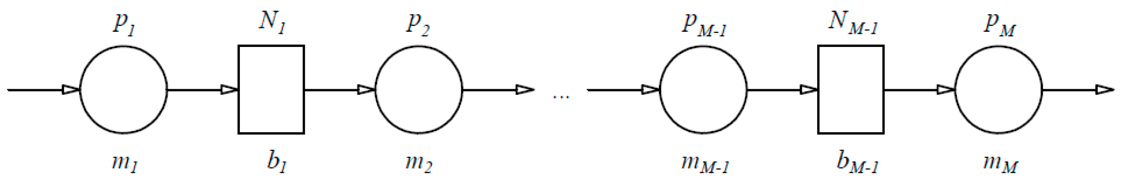
Mathematical models are the backbone of every approach exploited within the PSE framework. In this study, different approaches to the mathematical modeling of serial Bernoulli lines were considered and compared. To do this, it is convenient to depict a production line using circles, rectangles, and arrows representing machines, buffers, and material flow direction, respectively (
Figure 1). Each machine
mi, where
i = 1, 2, …,
M and
M is the total number of machines, has Bernoulli reliability, i.e., it is in the state {up} with the associated probability
pi and in the state {down} with probability 1-
pi. Every buffer
bi, where
i = 1, 2, …,
M − 1, is placed between two adjacent machines and is of the capacity
Ni, where
Ni ∈ ℕ
0. In addition to this, a usual set of assumptions applied in each of the models considered are as follows [
8]:
The status of each machine is determined independently from the status of other machines;
The status of each machine is determined at the beginning and the state of the buffer at the end of each time slot;
Failures are time-dependent;
The first machine is never starved, the last machine is never blocked.
Such a mathematical model can be considered using an analytical, semi-analytical, or numerical approach, while the main outputs of the evaluation usually focus on the Bernoulli serial line’s performance measures, namely, the production rate,
PR; the work-in-process at the
ith buffer,
WIPi; the probability of blockage of the
ith machine,
BLi; and the probability of starvation of the
ith machine,
STi [
8,
10]. The production rate,
PR, stands for the expected number of pieces per cycle time produced by the last machine and is defined as the intersection of events:
The work-in-process,
WIPi, as the average number of semi-products at the
ith buffer, is determined using the following relation:
where
hi (
i = 1, 2, …,
M − 1) is the number of semi-products at the
ith buffer and
is the steady-state probability of the system being in the state
h1h2h3…
hM−1. The average number of semi-products at the level of the complete line can be expressed using Equation (2):
Given the assumption that the last machine can never be blocked, the probability of blockage of the
ith machine
BLi is defined separately for the penultimate machine as the intersection of events:
while in the case of machines
m1,
m2, …,
mM−2, it is equal to
Finally, by taking into account the assumption that the first machine can never be starved, the probability of starvation of the
ith machine,
STi, is equal to the intersection of events that the
i-1 buffer is empty and that the subsequent machine is in the up state, i.e.,
2.1. The Analytical Approach
According to Equations (1)–(6), the key parameter yielding the performance measures is the steady-state probability
of a system being in the state
h1h2h3…
hM−1. Therefore, it is of great importance to enable its formulation. The first possibility is to use the analytical approach by solving the Chapman–Kolmogorov equations using an eigenvalue problem [
27]:
where [
P] and [
I] are the system’s transition matrix and the identity matrix, respectively;
is the first eigenvalue of the transition matrix; and {
P1} is the eigenvector associated with the first eigenvalue composed of the steady-state probabilities
. This problem can be solved by using the definition of a transition matrix via the multiplication of the constitutive matrices defined for each machine in the line, i.e.,
A detailed algorithm for the formulation of the constitutive matrices is available in [
10]. Unfortunately, the analytical approach quickly becomes rather cumbersome and CPU demanding, particularly as the system’s state space grows in the number of possible states. Therefore it is not applicable in cases such as when daily or weekly factory-floor analysis is required. However, it is extremely valuable in the case when the validation of semi-analytical or numerical approaches is required.
2.2. The Semi-Analytical Approach
2.2.1. The Finite-State Method
The finite state method is a recently developed method that bypasses the demanding CPU problem of the analytical solution by discretizing the system’s state space using the two-machine–one-buffer finite-state elements and the associated analytical solution. Here, we provide only a brief outline of the method as it is presented in detail in [
9].
The main idea of the finite state method is to discretize the system’s state space using the finite state elements that are defined concerning the weakest machine in the production line,
mm (
Figure 2). In such a way, a set of
m − 1 upstream and
M −
m downstream elements can be defined, depending on the properties of the serial production line. The total number of finite-state elements modeling the steady-state behavior of the Bernoulli serial line amounts to
M − 1. Each upstream element
e, where
e <
m, is composed of the machine
me, the weakest machine in the line
mm, and the buffer
be placed in between them. Similarly, each downstream element
e, where
m <
e <
M − 1, is formulated using the weakest machine in the line
mm, the machine
me, and the buffer
be placed in between them.
Once defined, a distribution of the steady-state probabilities can be expressed at the level of each finite-state element using a well-known analytical solution of the two-machine–one-buffer problem [
8] depending on the upstream and downstream arrangement. Such a distribution in the case of the upstream elements is equal to
where
e <
m − 1;
pe and
pm are the probabilities that machines
e and
m are in the state {up}, respectively;
Ne is the capacity of the buffer
be; and
ae =
pe (1 −
pm)/
pm(1 −
pe). In the same way, the steady-state distribution in the case of the downstream elements is equal to
where,
m <
e <
M − 1,
pe+1 is the probability that the machine
e + 1 is in the state {up}, and
ae =
pm (1 –
pe + 1)/
pe + 1 (1 −
pm). Finally, the distribution of the steady-state probabilities for a complete system can be approximated using the intersection of independent events at each buffer [
9], i.e.,
Once the distribution is known, all of the considered performance measures can be determined using Equations (1)–(6).
The main advantage of the finite state method as compared to the analytical approach is the significantly lower CPU requirement. To be more precise, the CPU requirement in the case of the analytical formulation of long lines can reach up to weeks or months, depending on the number of machines involved and the capacities of buffers. However, the same problem can be solved using the FSM approach in a matter of seconds, which is a considerable advantage. In addition to that, the FSM is the only available semi-analytical method that enables the recovery of the distribution of the steady-state probabilities, , along with the formulation of the performance measures.
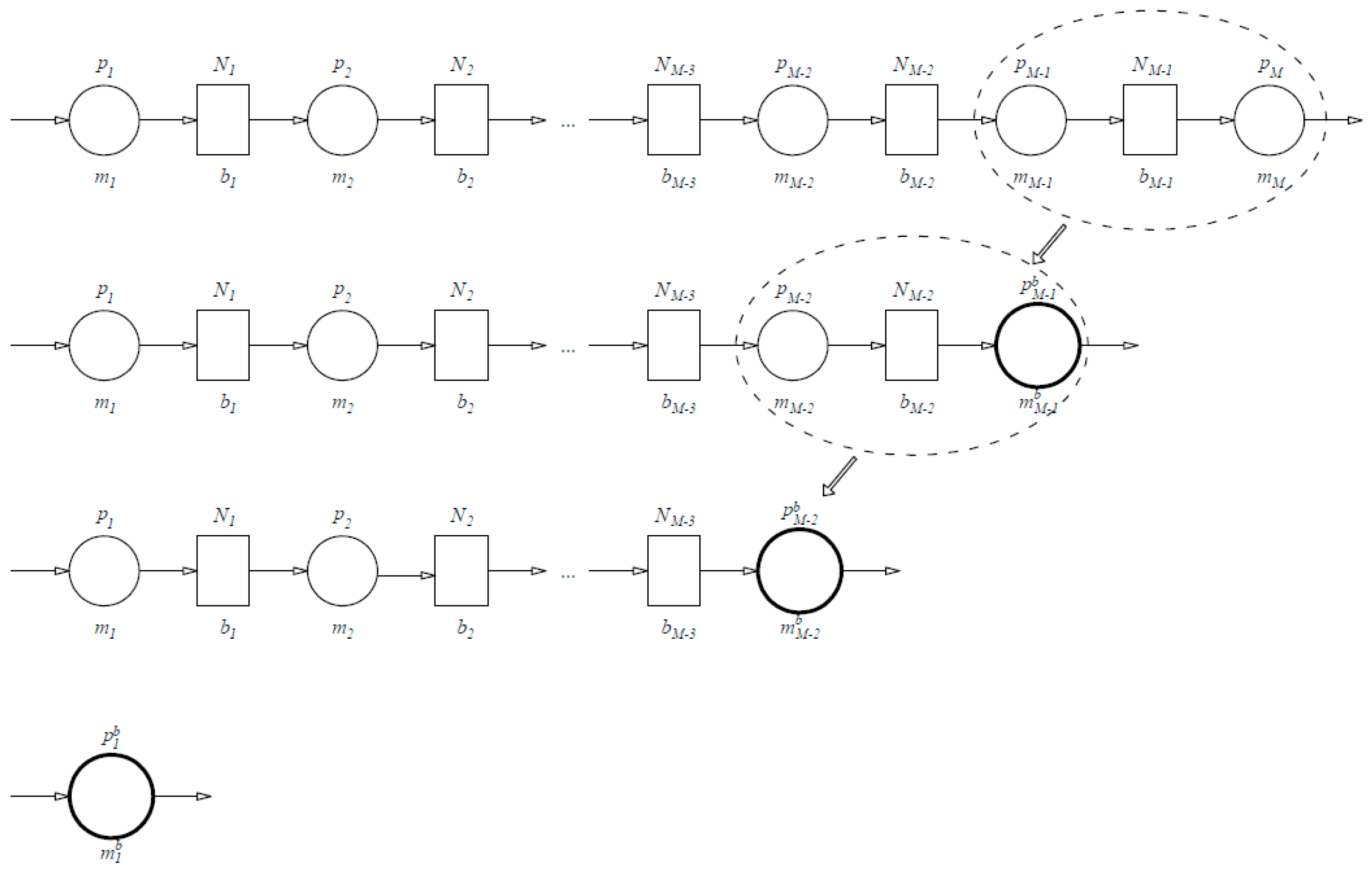
2.2.2. The Aggregation Procedure
The aggregation procedure is based on the application of the backward–forward aggregation algorithm lumping in a stepwise fashion to aggregate a complete production line into a single machine. As the first step, the machines
mM and
mM−1 and the buffer
bM−1 are aggregated into a new (virtual) machine
, where the superfix
b stands for ‘backward’. The reliability of the newly aggregated machine
is equal to the production rate (PR) determined using analytical expressions available in the two-machine–one-buffer case. In the next step, the machine
is used, along with the machine
mM−2 and buffer
bM−2, to create the new aggregated machine
with a reliability that is determined using the same analytical expressions as in the previous step. This procedure is repeated until the complete line is aggregated into a single machine
of the reliability
(
Figure 3).
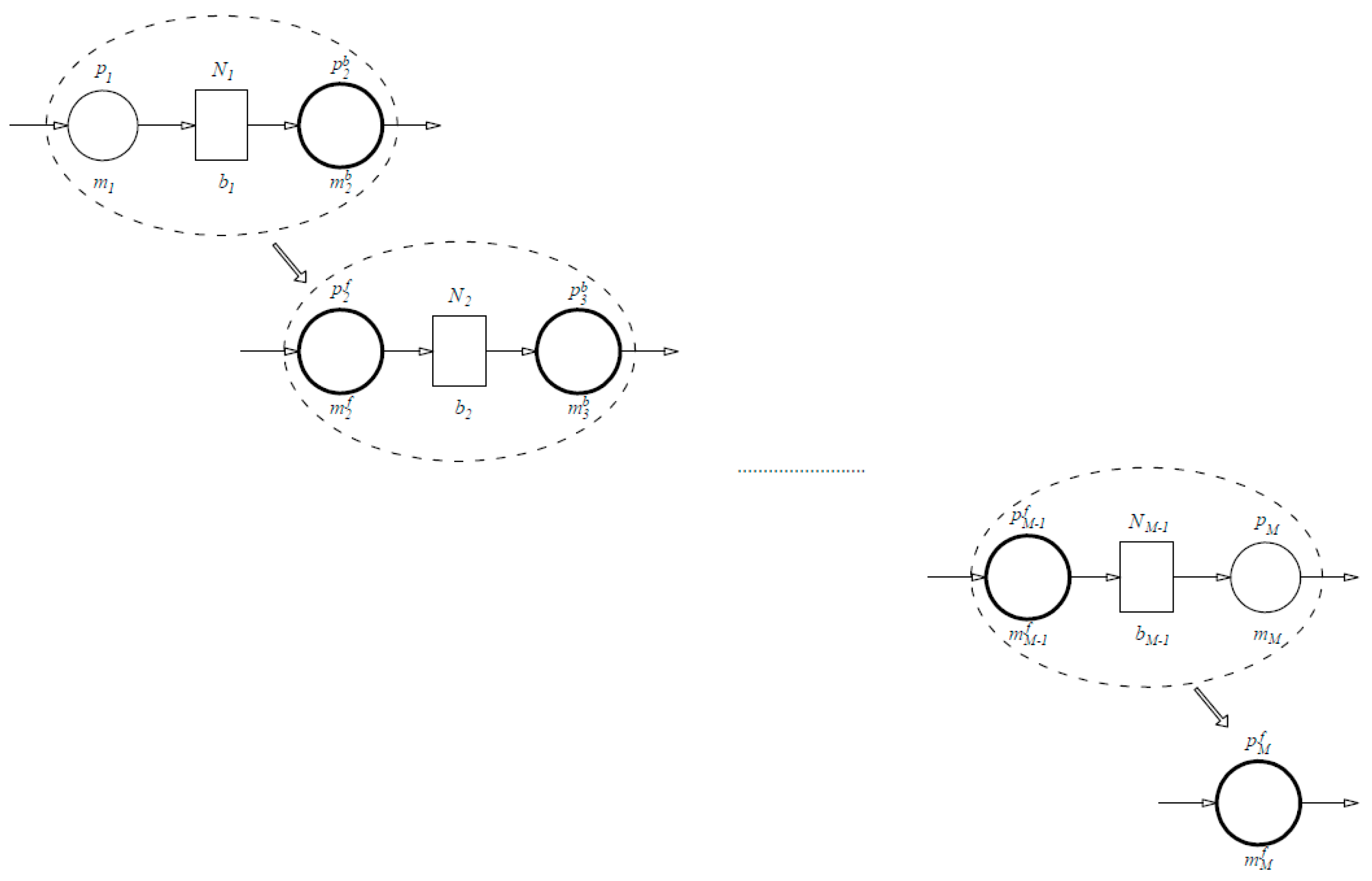
In the next stage, the algorithm aggregates the line from the beginning, starting with machine
m1, the machine of the backward aggregated rest of the line
, and the buffer
b1. Again, a new machine
, where
f stands for forward, is created with the associated reliability
. The same steps are thus repeated until the complete line is aggregated into a single machine
with reliability
(
Figure 4). Such a backward–forward algorithm is then iterated until the reliabilities
and
converge to the same value [
8].
Since the aggregation procedure does not provide complete information on the steady-state probability distribution
, the performance measures cannot be determined using Equations (1)–(6). However, the equivalent representation of the Bernoulli production line using a backward–forward algorithm enables the formulation of mathematical expressions used to estimate the performance measures. Here we provide only their summary, while their detailed derivation can be found in [
8].
The production rate (PR) of the serial Bernoulli production line can, therefore, be determined as follows:
where
and
Similarly, the work in process contained at the
ith buffer is equal to
where
i = 1, 2, …,
M − 1. Finally, the probabilities of blockage and starvation associated with a particular machine can be determined using
where
is given in Equation (13).
Again, the governing advantage of the aggregation procedure as compared with the analytical solution is the significantly lower CPU requirement. In such a way, the procedure enables a fast evaluation of the performance measures associated with the considered production line. Therefore, it is applicable in cases of daily or weekly analyses of production systems using the factory floor data. However, validation of both approximation methods (the finite state method and the aggregation procedure) is presently available in only several selected cases. Therefore, validation of their accuracy was the focus of the present study.
2.3. The Numerical Modeling
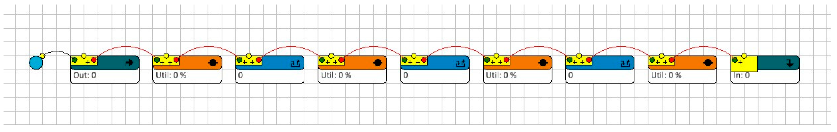
The numerical modeling of production systems usually relies on the application of discrete event simulation. Therefore, a similar approach will be used here to enable additional comparison and validation of the results. In this way, an additional data set obtained using the numerical approach will be provided, while the analytical approach remains the referent model used to validate all other approaches.
For modeling purposes, the simulation program Enterprise Dynamics 10.3 was used. The software deals with standard elements that represent devices and equipment in a production plant, such as machines, conveyors, cranes, forklifts, and warehouses. In the case of each production line, the simulation model is built up of the standard atoms: source, server, queue, and sink [
28]. The source atom is used to generate a piece per unit time entering the production line composed of server atoms representing the action of machines and requiring a cycle time set up (
Figure 5a). Additionally, the probability of a server being in the state {up}, respectively {down}, can be specified using features such as the mean time to failure (MTTF) and mean time to repair (MTTR) (
Figure 5b), where the MTTF represents the time when the machine is available, and MTTR represents the time when the machine is not available due to its failure. Since we are dealing with the Bernoulli production lines, the MTTF equals
pT, while the MTTR amounts to (1 −
p)
T, where
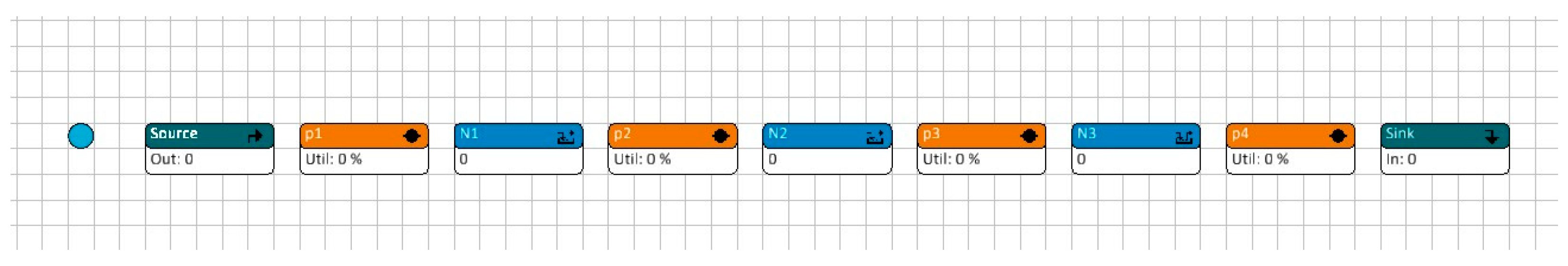
T is the cycle time that takes a unit value. Each buffer of the considered serial production line is modeled using a queue atom. Therefore, the feature capacity is set up to the maximum number of pieces for each buffer. Finally, the sink atom is used to count the number of products passing through the production line and, consequently, to determine the throughput of the line. An example of the numerical model of the serial Bernoulli production line composed of four machines is presented in
Figure 6, while the connection between atoms can be seen in
Figure 7.
3. Theoretical Examples and Results
The main goal of the present study was to validate the accuracy of the performance measures determined using the semi-analytical approaches, namely, the finite state method and the aggregation procedure, as well as the numerical method, against those obtained using the analytical approach in the case of the serial Bernoulli production line. To do that, a set of theoretical examples was created in the case of lines composed of 3–9 machines. In each case, 200 lines were generated to retrieve a reliable estimate of the accuracy of each method considered. Therefore, a total of 1400 different lines were taken into account. On the other hand, lines involving more than nine machines were not considered here as the CPU requirements for the analytical evaluation of the problem surpassed, in most cases, the possibilities of standard personal computers. Therefore, the largest number of possible system states, i.e., the unknown steady-state probabilities, constituting the considered system state space was limited to 100,000 per line.
The scale of the system state space was determined as a product and is a function of both the total number of buffers M − 1 and their capacity Ni. Consequently, the same state space scale can be associated with the short line of the significant buffering capacity, as well as with the long line of the relatively small buffering capacity. Therefore, the scale of the system state space was considered relevant in the course of the accuracy validation. Furthermore, since we were dealing with the steady-state probability distributions, all of the conclusions drawn from the considered theoretical examples can be extended to longer serial Bernoulli production lines.
The properties of each line, namely, the reliability of machines and the capacity of buffers, were determined using a random number generator assigning a reliability
pi = rand (0.5, 1) to each machine and capacity
Ni = rand (1, 10) to each buffer. The total capacity of buffers was conditioned to
. All of the formulated lines were subsequently analyzed using an in-house Fortran-based program ProLab [
29] and data on the performance measures was generated using the analytical solution (Equations (1)–(6) and (8)), FSM (Equations (1)–(6) and (11)), and the aggregation procedure (Equations (12)–(16)). Extensive data, including the properties of the considered lines and performance measures obtained using three different methods, is provided in
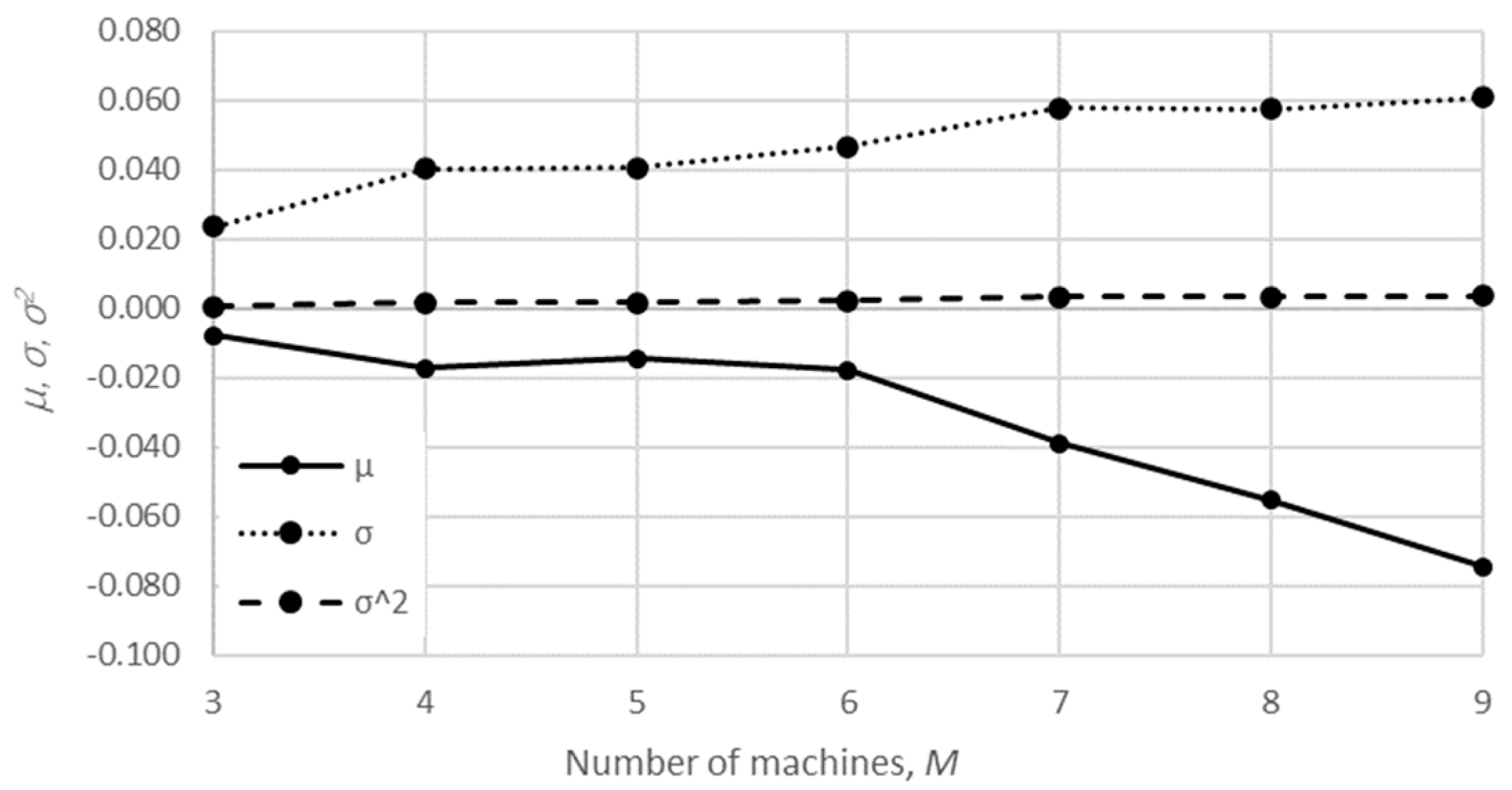
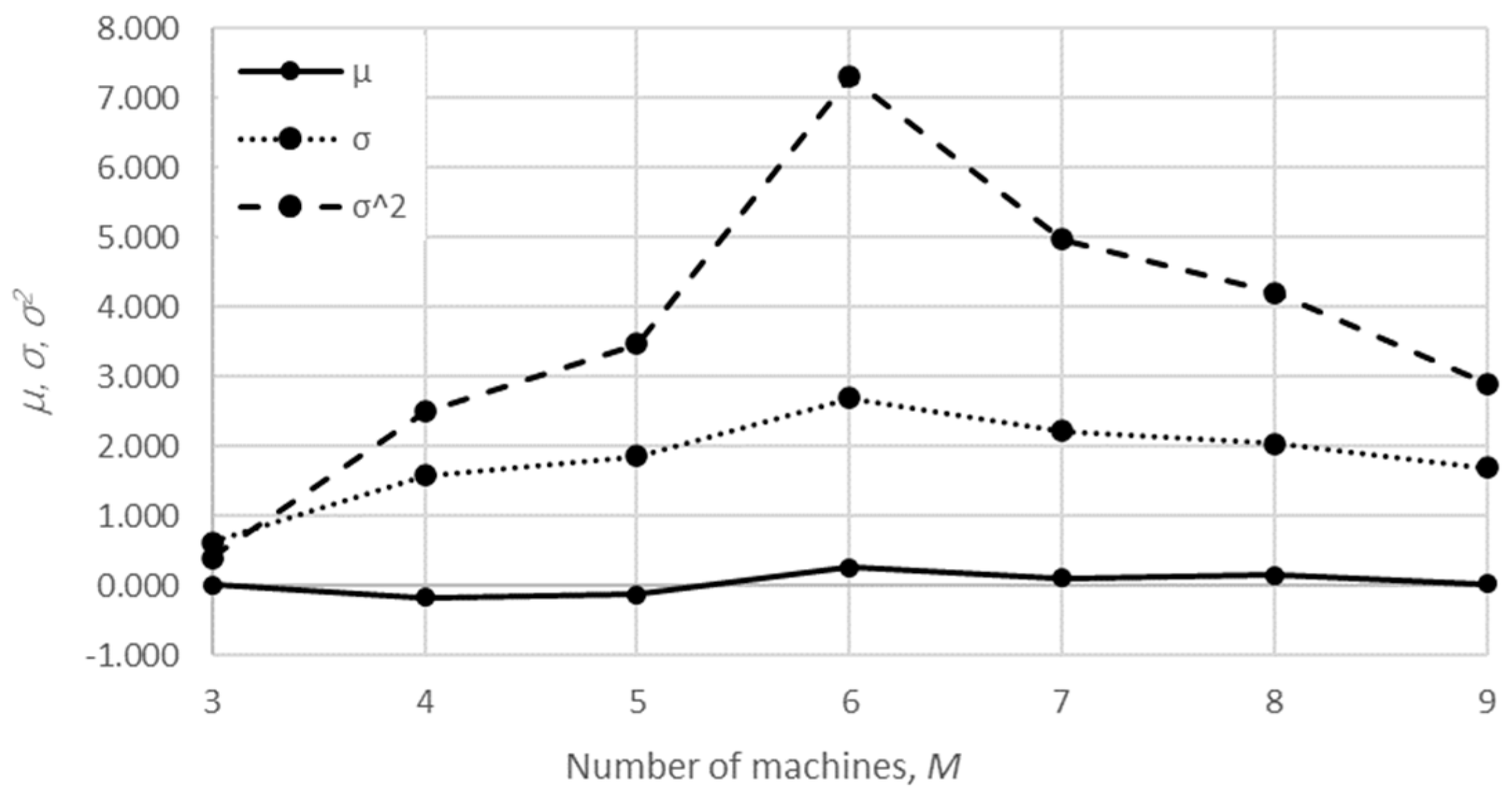
Supplementary Materials S1. Here, only a summary of the obtained results is presented in
Table 1 and
Table 2 in a form of the mean value
μ, standard deviation σ, and variance σ
2 of the relative error, which were determined for the analytical solution in the case of each performance measure. For example, a mean value
of the relative error obtained in the case of the production rate (PR) determined using the aggregation procedure (AGG) is equal to
where
PRA and
PRAGG are the production rates determined using the analytical approach (A) and the aggregation procedure (AGG), respectively, and
NL is the total number of the randomly generated lines per each case considered (lines composed of 3–9 machines). In each case,
NL is equal to 200. Similarly, the standard deviation and the variance of the relative error are equal to
The mean value, the standard deviation, and the variance of the relative error are presented in
Table 1 and
Table 2 and
Figure 8,
Figure 9,
Figure 10 and
Figure 11 in the case of the semi-analytical methods, along with all of the considered performance measures, namely, the production rate (
PR), the total work-in-process (
WIP), the probability of blockage of the ith machine (
BLi), and the probability of starvation of the machine
i (
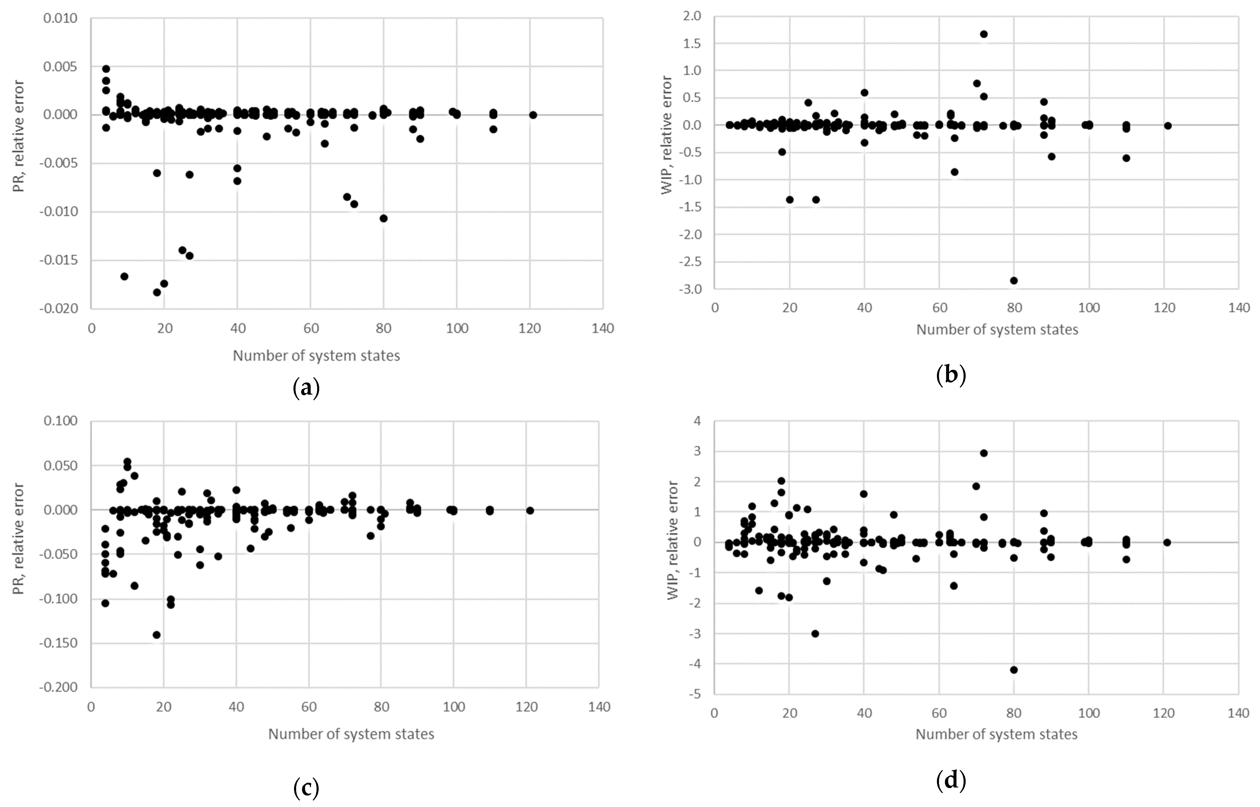
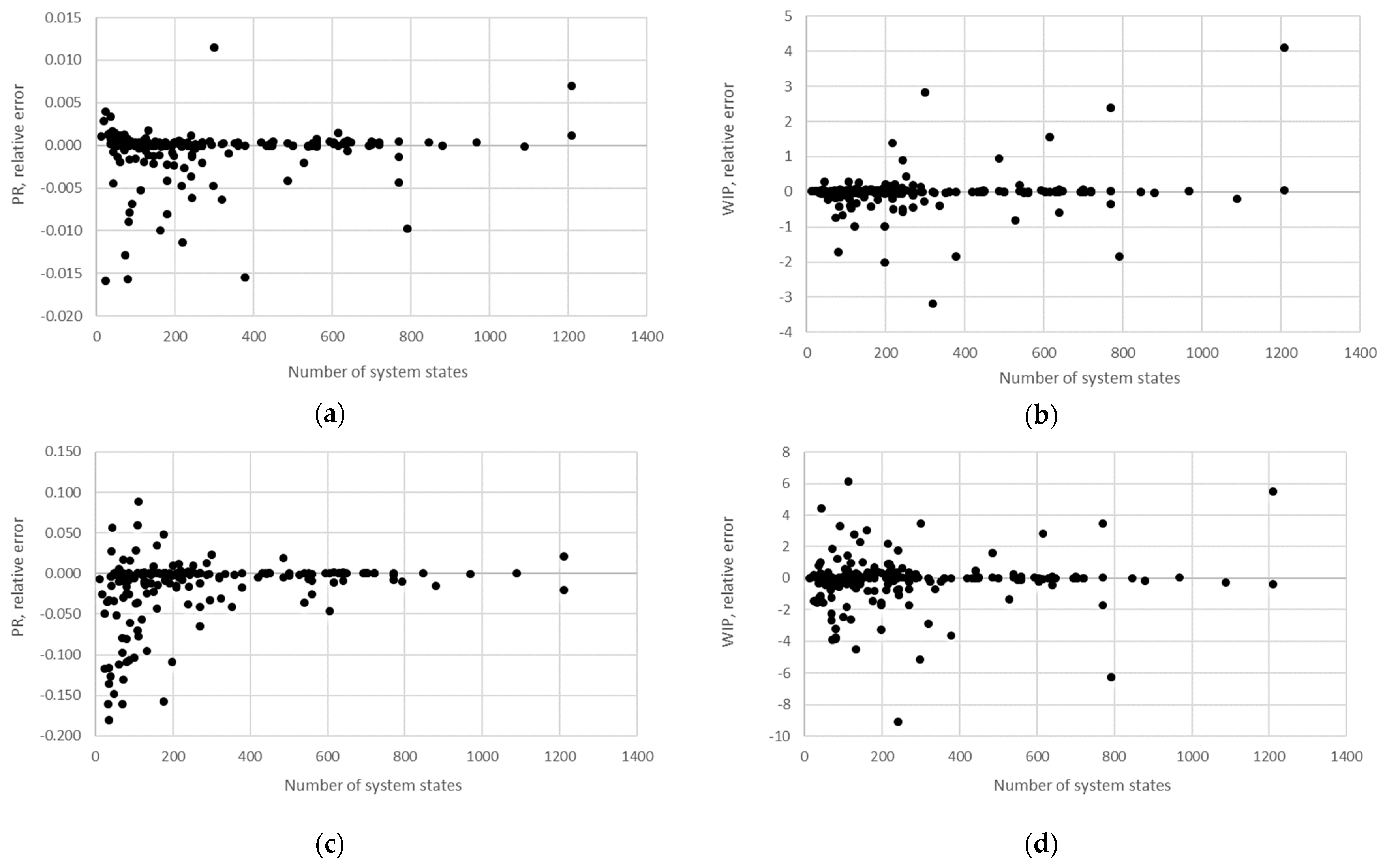
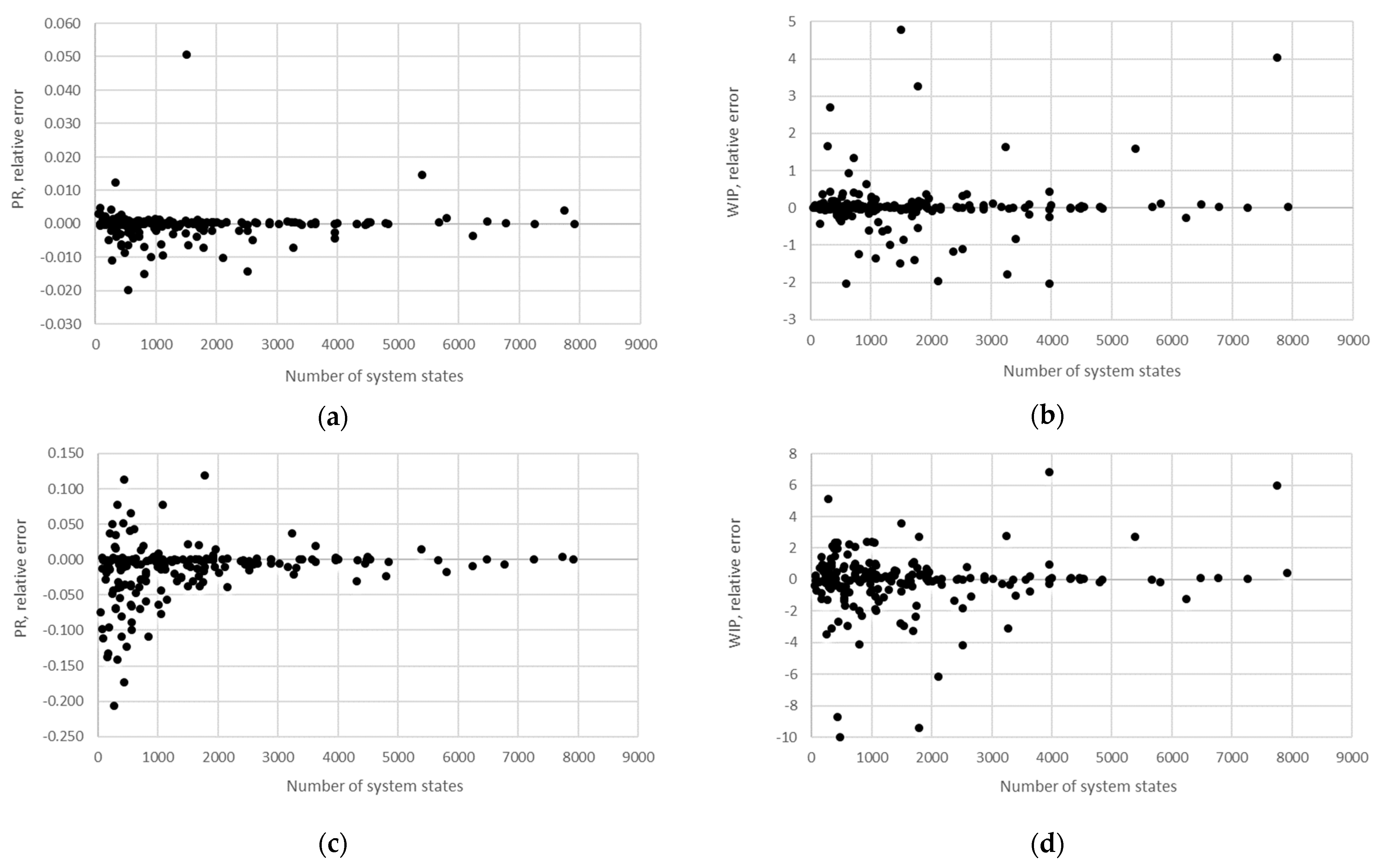
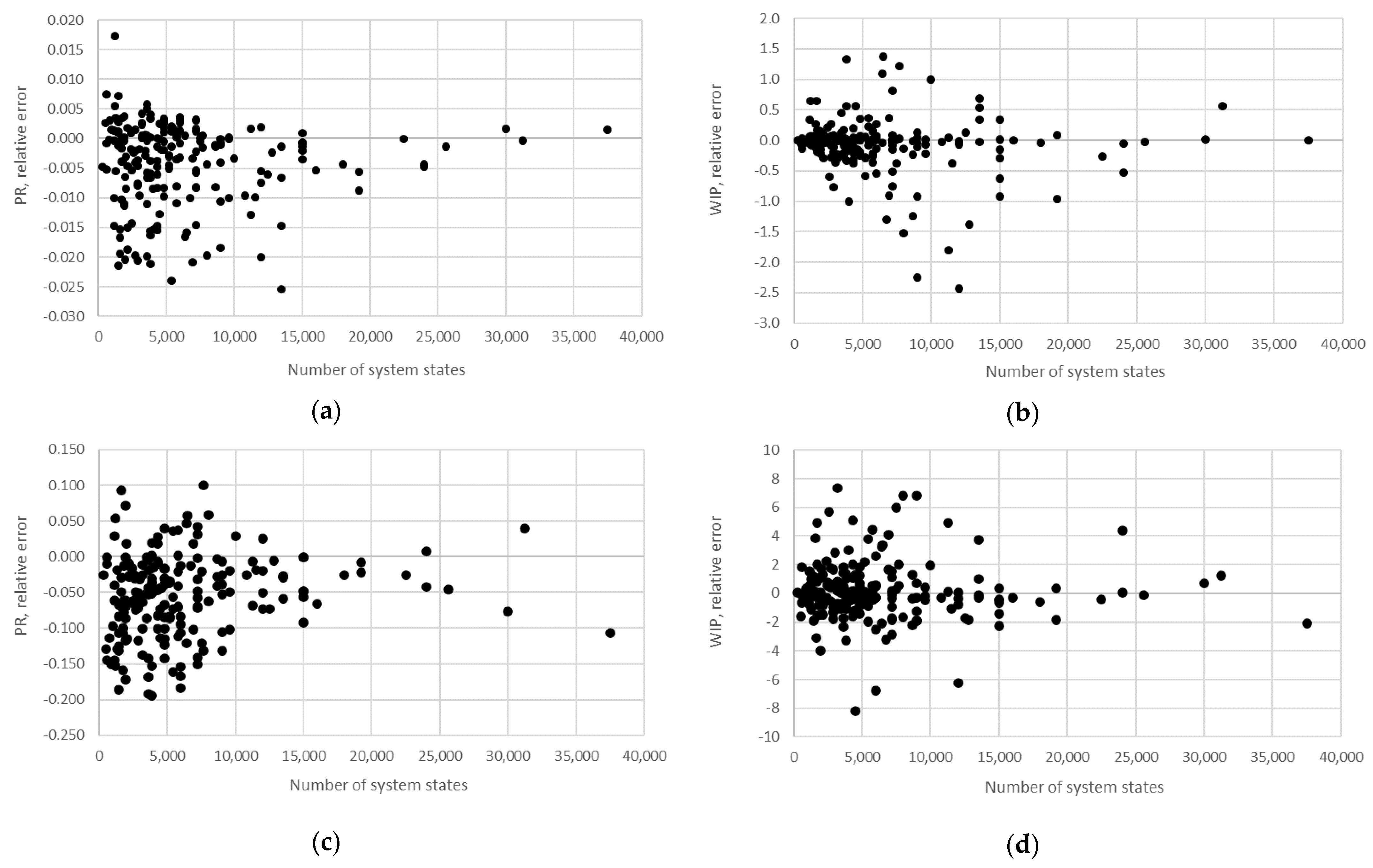
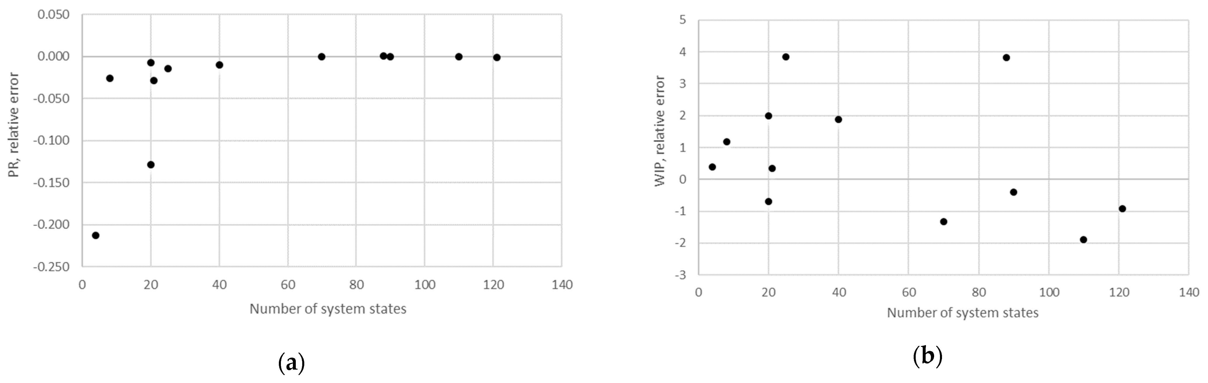
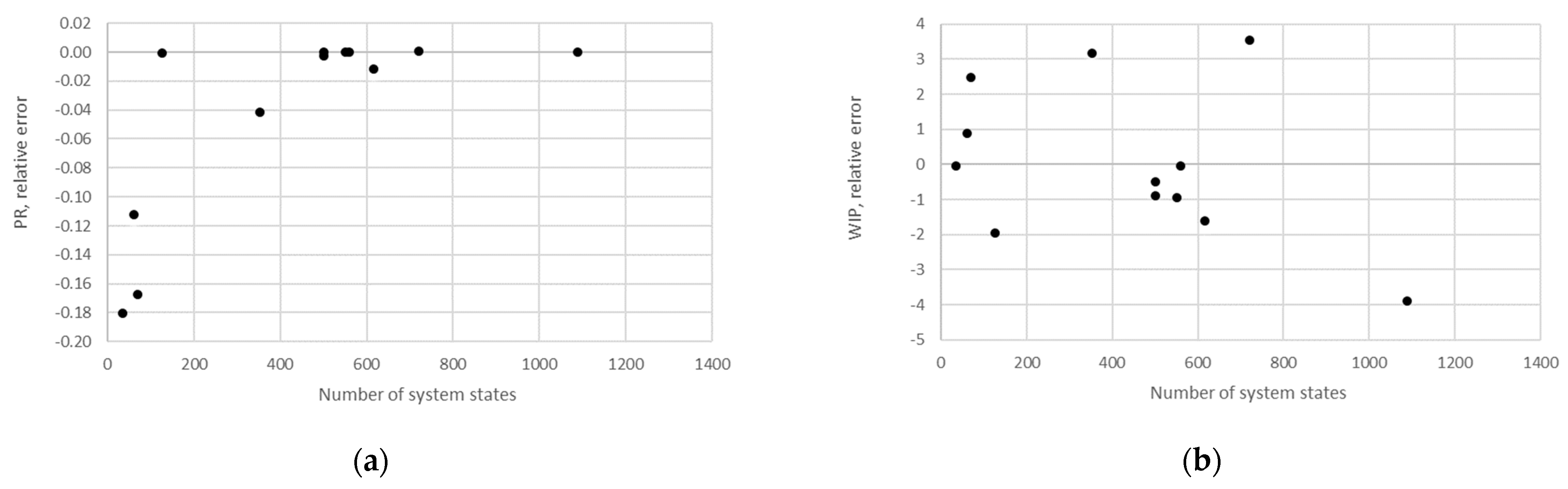
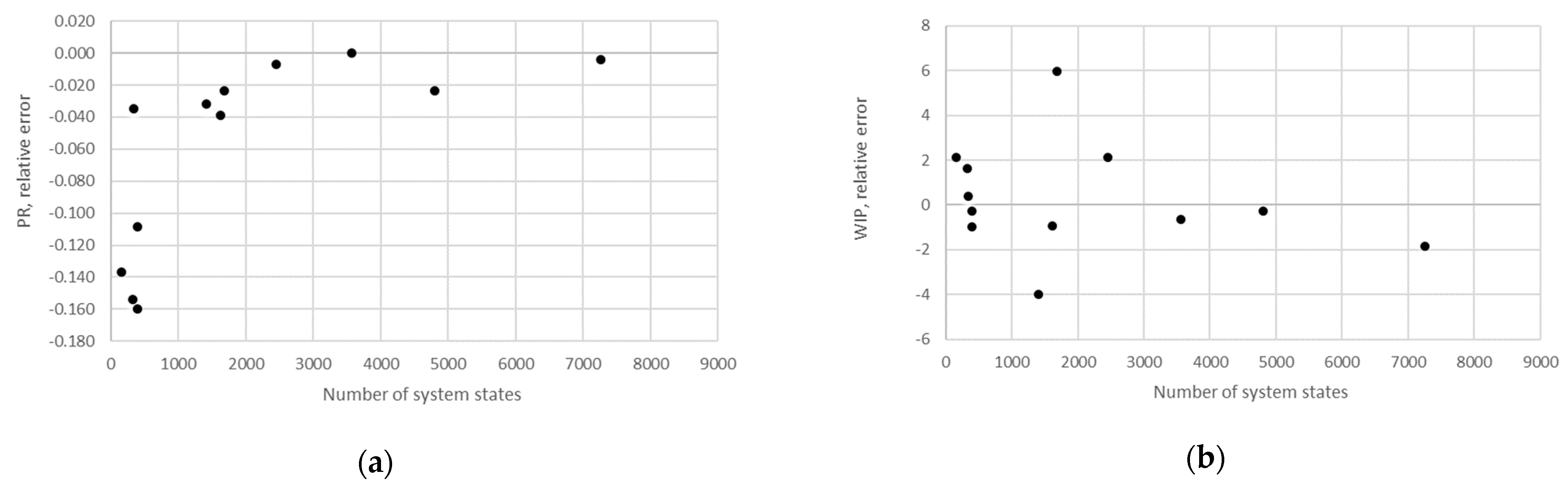
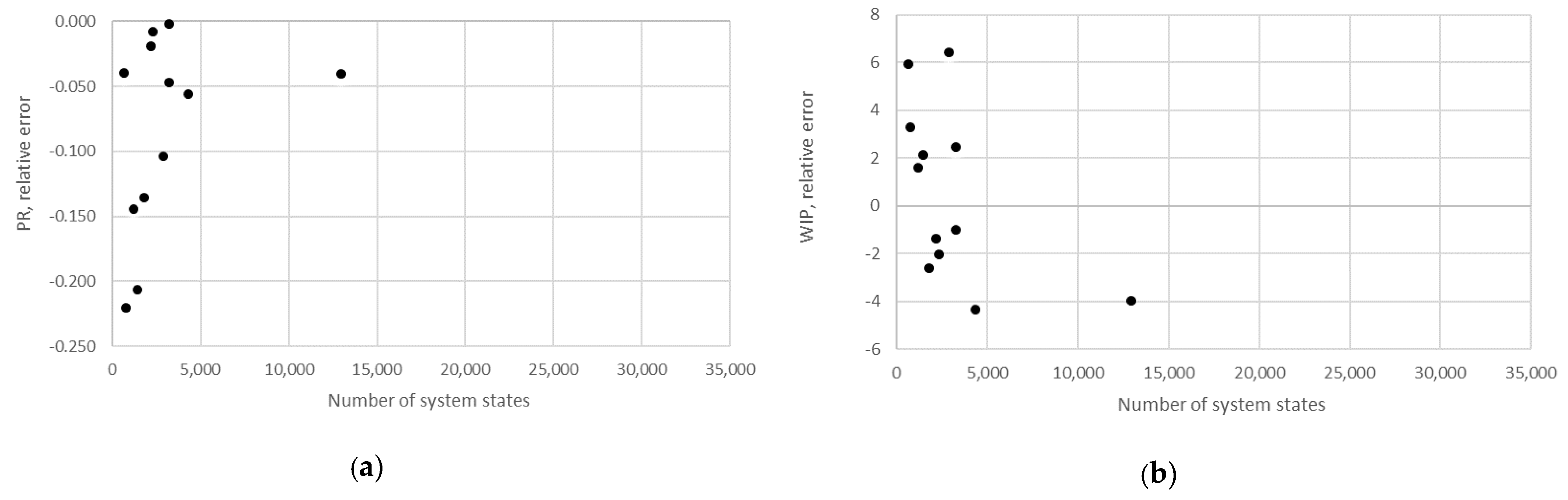
STi). Furthermore, the relative error obtained using the aggregation procedure and the finite state method in the case of production rate and the total work in process concerning the state space scale of each line is presented in
Figure 12,
Figure 13,
Figure 14,
Figure 15,
Figure 16,
Figure 17 and
Figure 18.
The numerical method was validated in the same way. However, the number of considered cases had to be reduced as the recovery of the results turned out to be quite demanding, particularly regarding the work in process. Therefore, 12 production lines were sampled out of the previously generated 200 different possibilities for each case considered. The sampling criteria were based on the performance measures obtained using the analytical approach. In this way, the following lines were identified:
Line 1: line with the smallest PR;
Line 2: line with the largest PR;
Line 3: line with the PR in between the production rates of lines 1 and 2;
Line 4: line with the smallest WIP;
Line 5: line with the largest WIP;
Line 6: line with the WIP in between the work in process of lines 4 and 5;
Line 7: line with the smallest BLM−1;
Line 8: line with the largest BLM−1;
Line 9: line with the BLM−1 in between the probabilities of blockage of lines 7 and 8;
Line 10: line with the smallest STM;
Line 11: line with the largest STM;
Line 12: line with the STM in between the probabilities of starvation of lines 10 and 11.
Consequently, a total of 84 lines were modeled using the discrete event simulation software Enterprise Dynamic 10.3 [
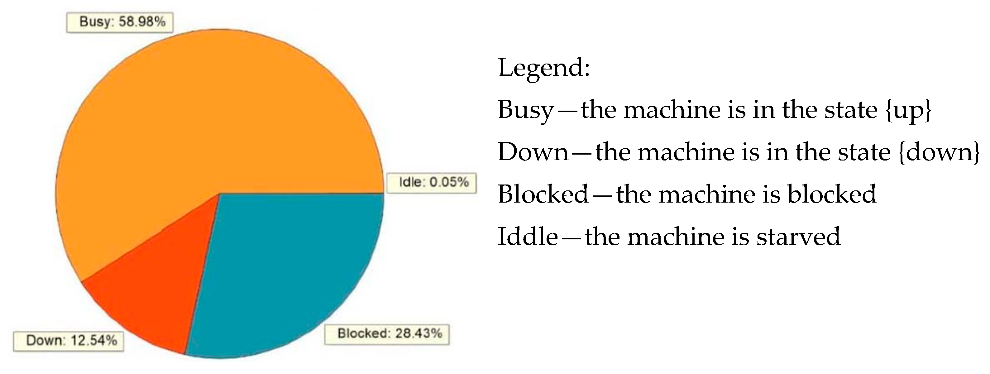
30]. The reliability data, as well as the capacity of the buffers, were set to values corresponding to the properties of the selected lines. Additionally, to model the selected theoretical examples, the cycle time of each machine was set to a unit value. Similarly, the capacity of the source atom was equal to one unit per cycle time. The simulation running time was set to 36,000 s and each simulation was carried out once for each production line, as the machine reliability data did not change during the simulation. Transient effects of the considered production systems diminished quite soon after simulation initialization as the cycle time took a unit value. Therefore, the warm-up period of each simulation could be neglected as its share in the total simulation running time was below 0.02%. An example of the simulation output results in the case of one selected machine is given in
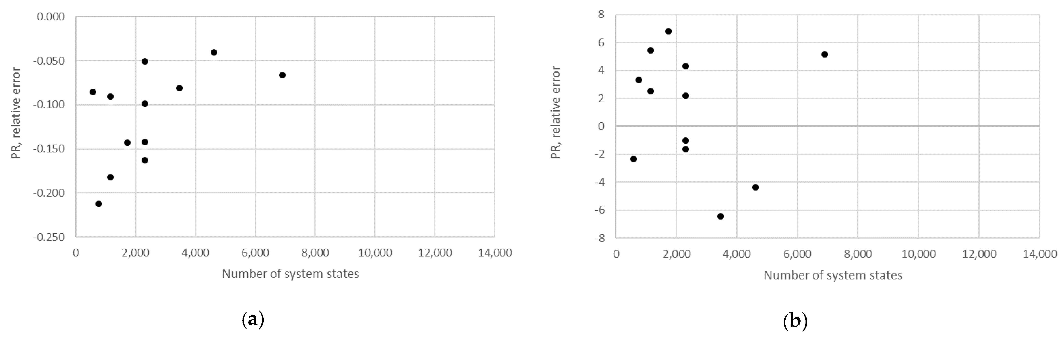
Figure 19. In this way, a validation of the numerical method was enabled as an evaluation of the relative error determined concerning the analytical solution for each serial Bernoulli production line. A summary of the obtained results is presented in
Table 3 and
Figure 20 and
Figure 21, while extensive data, including properties of the considered lines and performance measures obtained using the numerical method, are provided in
Supplementary Materials S1. In addition, the relative error obtained using the numerical method in the case of the production rate and the total work in process concerning the state space scale of each line is presented in
Figure 22,
Figure 23,
Figure 24,
Figure 25,
Figure 26,
Figure 27 and
Figure 28.
Discussion
The obtained results demonstrate that all of the considered methods, i.e., the aggregation procedure, FSM, and the numerical modeling, quite accurately represented the steady-state behavior of the serial Bernoulli production lines, particularly regarding the production rate and the probabilities of blockage and starvation. In these cases, all of the discrepancies could be considered negligible in terms of the mean value, standard deviation, and variance. This was also valid for the relative error distribution concerning the number of system states obtained in the case of PR, where most of the considered cases yielded almost the exact solution.
Some discrepancies related to the work-in-process performance measures could be detected in all cases as a direct consequence of the amplification of the error at the level of the steady-state probability through Equations (2) and (3). Furthermore, it can be seen that the relative error concerning the WIP was slightly higher in the case of FSM as compared to the aggregation procedure. This issue is a consequence of a relatively rough discretization of the state spaces related to the lines of rather small buffering capacities. The most significant discrepancies were related to the WIP determined using the numerical model. These discrepancies, both in terms of the mean value and data variation, were a direct consequence of the round-off procedure of the simulation program when determining the number of pieces contained at each buffer.
Concerning the CPU requirements, the semi-analytical methods required the least processing time (less than one second, regardless of the number of system states) and are therefore suitable for further development and implementation within more complex data structures dealing with lean design or improvability issues. On the other hand, the analytical method, although accurate and robust, required substantial amounts of processing time, which in some cases, reached up to several weeks. The order of magnitude of the CPU requirements in the case of the analytical method could be estimated as , quickly taking quite significant values that are highly impractical for further considerations dealing with the design of the production systems. Finally, the numerical method, although requiring a low CPU time, requires a dedicated and educated operator skilled in result interpretation and quick adjustments of the existing numerical models.
The considered examples, although theoretical, represent an excellent and valuable collection of the benchmark Bernoulli serial production lines, which can be employed in future research and development of the PSE tools. Unfortunately, a set of the considered lines could not be consistently extended to production lines involving more than six machines, as the analytical solution of the problem would become elusive in some, if not most, of the cases. However, this does not diminish the main findings of this research and their extension to the modeling of real production lines. Finally, both of the considered semi-analytical methods can be employed without limitation for the evaluation of the performance measures across various serial production systems employing machines with Bernoulli reliability.
4. Conclusions
The manufacturing industry has a significant impact on the economic growth of countries. Therefore, it is of crucial importance to make it more competitive and profitable. One possibility in that sense is to apply the systematic approach developed by the PSE research community and based on the mathematical modeling of real-life production systems. This study has considered three possible approaches to the mathematical modeling of a Bernoulli serial production line’s steady-state behavior, namely, the analytical, semi-analytical, and numerical approaches, where the semi-analytical approach focused on the application of the aggregation procedure and the recently developed FSM. A brief outline of the considered models was provided to enable accuracy validation against the performance measures obtained using the analytical model.
All of the considered models proved to be sufficiently accurate, particularly regarding the production rate, the probability of blockage, and the probability of starvation. Some discrepancies were detected in the case of the work-in-process data, mainly due to round-off errors in the case of the numerical model or due to relatively rough discretization of small state spaces in the case of FSM. Concerning the CPU requirements, all of the methods, except the analytical approach, were shown to be rapid methods that yielded the evaluation results in a matter of seconds, while the analytical approach required a substantial evaluation time, sometimes reaching up to several weeks. Therefore, the semi-analytical and numerical methods can be recommended for further application, while substantial effort has to be made to reduce the CPU requirements of the analytical approach.
Further research concerning the mathematical modeling of the production systems should focus on the development, validation, and application of the analytical and semi-analytical models of more complex systems, including splitting lines, assembly systems, systems with quality check, and rework stations, where both models concern synchronous and asynchronous cases. Such a demanding task can only be accomplished if a systematic approach to the PSE is applied.


