Supervised Classification of Diseases Based on an Improved Associative Algorithm

Abstract

The linear associator is a classic associative memory model. However, due to its low performance, it is pertinent to note that very few linear associator applications have been published. The reason for this is that this model requires the vectors representing the patterns to be orthonormal, which is a big restriction. Some researchers have tried to create orthogonal projections to the vectors to feed the linear associator. However, this solution has serious drawbacks. This paper presents a proposal that effectively improves the performance of the linear associator when acting as a pattern classifier. For this, the proposal involves transforming the dataset using a powerful mathematical tool: the singular value decomposition. To perform the experiments, we selected fourteen medical datasets of two classes. All datasets exhibit balance, so it is possible to use accuracy as a performance measure. The effectiveness of our proposal was compared against nine supervised classifiers of the most important approaches (Bayes, nearest neighbors, decision trees, support vector machines, and neural networks), including three classifier ensembles. The Friedman and Holm tests show that our proposal had a significantly better performance than four of the nine classifiers. Furthermore, there are no significant differences against the other five, although three of them are ensembles.

1. Introduction

This paper proposes a novel machine learning algorithm that is successfully applied in medicine [1]. In this context, it is pertinent to mention that in machine learning, there are four basic tasks corresponding to two paradigms. The unsupervised paradigm includes the clustering task, while the remaining three tasks belong to the supervised paradigm: classification, recalling, and regression [2].

The novel machine learning algorithm proposed in this article involves two of the three tasks of the supervised paradigm: classification and recalling. The classification task consists of assigning, without ambiguity, the class that corresponds to a test pattern. For example, a classification algorithm could support a physician with a certain percentage of success if a chest X-ray corresponds to a patient suffering from COVID-19 or pneumonia. The hit rate of the classifier will depend on how complex the dataset is, as well as the quality of the machine learning algorithm [3].

Recalling is the second machine learning task involved in this proposal. Unlike the classification task in which a label is assigned to a pattern, the recalling task is responsible for assigning another pattern to the test pattern. In the example above, when having a chest X-ray as a test pattern, the recalling task tries to associate this test pattern with another pattern, such as with the patient’s social security number. Associative memories are the algorithms that carry out the recalling task [4].

The central part of the machine learning algorithm proposed in this paper consists of carrying out the classification of diseases through an associative memory. In other words, we have converted an associative memory (whose natural task is recalling) into a classifier of patterns related to healthcare and, specifically, diseases.

The associative memory used here is the linear associator, a model that dates back to 1972 and whose development is attributed to two scientists working simultaneously and independently: Kohonen in Finland [5] and Anderson in the US [6].

The linear associator is a classic associative memory model. Its importance lies in the fact that it is one of the pioneering models in this branch of research. In relation to this model, studies have been carried out on convergence [7] and on its performance [8].

However, due to the low performance exhibited by this model in most of the datasets, very few applications have been published [9]. Researchers have dedicated efforts to improve the performance of the linear associator by preprocessing the data under study, with very modest advances [10,11].

The reason for the low success of the methods that seek to improve performance is that the linear associator requires a very strong restriction to the patterns in order for them to be recovered correctly. Vectors are required to be orthonormal. Given this, some researchers have tried to use the Gram–Schmidt orthogonalization process, which creates orthogonal projections for the vectors that are presented to it [12]. However, this solution has serious drawbacks [13]. This paper presents a proposal that does not use the Gram–Schmidt process, but rather a powerful mathematical tool: singular value decomposition [14,15].

The rest of the paper is organized as follows. Section 2 consists of three subsections, where the linear associator, its use as a pattern classifier, and in addition, the singular value decomposition are briefly described and exemplified. In Section 3, the central proposal of this paper will be described in detail. Section 4 is very important because it describes the datasets and the classification algorithms against which our proposal will be compared. Additionally, the experimental results are presented and discussed. Finally, in Section 5, the conclusions and future works are offered.

2. Related Methods

This section consists of three subsections. Section 2.1 describes the model that has been taken as the basis for this paper: the linear associator. Section 2.2 describes and exemplifies the possible use of the linear associator as a pattern classifier. In addition, some reflections on its advantages and disadvantages are discussed. On the other hand, Section 2.3 contains a brief description of the singular value decomposition, which is a powerful mathematical tool that strongly supports the central proposal of this paper. A wealth of illustrative numerical examples is presented across the three subsections.

2.1. Linear Associator

The linear associator requires a dataset $D$ that consists of ordered pairs of patterns (also called associations) whose components are real numbers. The first element of each association is an input column pattern, while the second element is the corresponding output column pattern [5,6]. By convention, the three positive integers $p,m,n$ facilitate symbolic manipulation. The symbol $p$ represents the number of associations, such that

$$D=\left\{\left(x^{\mu },y^{\mu }\right)|\mu =1,2,\dots ,p\right\}$$

(1)

In addition, $n$ and $m$ represent the dimensions of the input and output patterns, respectively, so that the $\mu$th input pattern and the $\mu$th output pattern are expressed as follows:

$$x^{\mu }={\left(x_1^{\mu },x_2^{\mu },\dots ,x_n^{\mu }\right)}^t=\left(\begin{array}{c}{x}_1^{\mu }\\ x_1^{\mu }\\ ⋮\\ x_n^{\mu }\end{array}\right)\in {ℝ}^n;y^{\mu }={\left(y_1^{\mu },y_2^{\mu },\dots ,y_m^{\mu }\right)}^t=\left(\begin{array}{c}{y}_1^{\mu }\\ y_2^{\mu }\\ ⋮\\ y_m^{\mu }\end{array}\right)\in {ℝ}^m$$

(2)

The linear associator algorithm consists of two phases: the training (or learning) phase and the recalling phase. To carry out these two phases, the dataset $D$ is partitioned into two disjoint subsets: a training or learning set $L$ and a test set $T$.

For each training couple of patterns $\left(x^{\mu },y^{\mu }\right)$, the matrix that represents its association is calculated with the outer product:

$$y^{\mu }·{\left(x^{\mu }\right)}^t=\left(\begin{array}{c}{y}_1^{\mu }\\ y_2^{\mu }\\ ⋮\\ y_m^{\mu }\end{array}\right)·\left(x_1^{\mu },x_2^{\mu },\dots ,x_n^{\mu }\right)=\left(\begin{array}{cccccc}{y}_1^{\mu }{x}_1^{\mu }& y_1^{\mu }{x}_2^{\mu }& \cdots & y_1^{\mu }{x}_j^{\mu }& \cdots & y_1^{\mu }{x}_n^{\mu }\\ y_2^{\mu }{x}_1^{\mu }& y_2^{\mu }{x}_2^{\mu }& \cdots & y_2^{\mu }{x}_j^{\mu }& \cdots & y_2^{\mu }{x}_n^{\mu }\\ ⋮& ⋮& & ⋮& & ⋮\\ y_i^{\mu }{x}_1^{\mu }& y_i^{\mu }{x}_2^{\mu }& \cdots & y_i^{\mu }{x}_j^{\mu }& \cdots & y_i^{\mu }{x}_n^{\mu }\\ ⋮& ⋮& & ⋮& & ⋮\\ y_m^{\mu }{x}_1^{\mu }& y_m^{\mu }{x}_2^{\mu }& \cdots & y_m^{\mu }{x}_j^{\mu }& \cdots & y_m^{\mu }{x}_n^{\mu }\end{array}\right)$$

(3)

If $l$ is the cardinality of $L$, then $l<p$, and $l$ matrices will be generated, which will be added to obtain the matrix $M$ that represents the linear associator.:

$$M={\displaystyle \sum }_{\mu =1}^l{y}^{\mu }·{\left(x^{\mu }\right)}^t={\left[m_{ij}\right]}_{m\times n}$$

(4)

The previous expression shows the trained memory, where the ijth component of M is expressed as follows:

$$M_{ij}={\displaystyle \sum }_{\mu =1}^l{y}_i^{\mu }{x}_j^{\mu }$$

(5)

Once the memory is trained, the recalling phase takes place. For this, the product of the trained memory with a test pattern x^ω is performed:

$$M·x^{\omega }=\left[{\displaystyle \sum }_{\mu =1}^l{y}^{\mu }·{\left(x^{\mu }\right)}^t\right]·x^{\omega }$$

(6)

Ideally, Equation (6) should return the output pattern $y^{\omega }$. In the specialized literature, it is not possible to find theoretical results that establish sufficient conditions to recover, in all cases, the output pattern $y^{\omega }$ from the input pattern $x^{\omega }$.

However, it is possible to use the well-known resubstitution error mechanism in order to establish the recovery conditions for the patterns in the learning set; that is, the memory will be tested with the patterns of the learning set. The following theorem establishes the necessary and sufficient conditions for this to occur.

Theorem 1.

Let M be a linear associator which was built from the learning set $D$ by applying Equation (4), and let $\left(x^{\omega },y^{\omega }\right)$ be an association in $D$. Then, the output pattern $y^{\omega }$ is correctly retrieved from the input pattern $x^{\omega }$ if and only if all input patterns are orthonormal.

Proof. 

Given that in the set $D$ there are $p$ associations, by applying Equation (4), we obtain $M$:

$$M={\displaystyle \sum }_{\mu =1}^p{y}^{\mu }·{\left(x^{\mu }\right)}^t$$

We will try to retrieve the output pattern and, by applying Equation (6), we find

$$M·x^{\omega }=\left[{\displaystyle \sum }_{\mu =1}^p{y}^{\mu }·{\left(x^{\mu }\right)}^t\right]·x^{\omega }$$

$$M·x^{\omega }=\left[y^1·{\left(x^1\right)}^t+y^2·{\left(x^2\right)}^t+\cdots +y^{\omega }·{\left(x^{\omega }\right)}^t+\cdots +y^p·{\left(x^p\right)}^t\right]·x^{\omega }$$

$$M·x^{\omega }=\left[y^1·{\left(x^1\right)}^t\right]·x^{\omega }+\cdots +\left[y^{\omega }·{\left(x^{\omega }\right)}^t\right]·x^{\omega }+\cdots +\left[y^p·{\left(x^p\right)}^t\right]·x^{\omega }$$

$$M·x^{\omega }=y^1·\left[{\left(x^1\right)}^t·x^{\omega }\right]+\cdots +y^{\omega }·\left[{\left(x^{\omega }\right)}^t·x^{\omega }\right]+\cdots +y^p·\left[{\left(x^p\right)}^t·x^{\omega }\right]$$

$$M·x^{\omega }=y^{\omega }·\left[{\left(x^{\omega }\right)}^t·x^{\omega }\right]+{\displaystyle \sum }_{\mu \ne \omega }{y}^{\mu }·\left[{\left(x^{\mu }\right)}^t·x^{\omega }\right]$$

Therefore, the right term will be ${\mathrm{y}}^{\mathsf{\omega }}$ if and only if two conditions are met:

$${\left(x^{\omega }\right)}^t·x^{\omega }=1and{\displaystyle \sum }_{\mu \ne \omega }{y}^{\mu }·\left[{\left(x^{\mu }\right)}^t·x^{\omega }\right]=0$$

In other words, ${\left(x^{\omega }\right)}^t·x^{\omega }=0$ and $y^{\mu }·\left[{\left(x^{\mu }\right)}^t·x^{\omega }\right]\forall \mu \ne \omega$.

These conditions are met if and only if the input vectors are orthonormal. □

In order to illustrate the operation of both phases of the linear associator, it is pertinent to follow each of the algorithmic steps through a simple example. In order for the example to satisfy the hypothesis of Theorem 1, it is assumed that the training or learning phase is performed with the complete dataset and that the trained memory is tested with each and every one of the dataset patterns; that is, $L=D=T$. In the specialized literature, this method is known as the resubstitution error calculation [16].

The example consists of three pairs of patterns, where the input patterns are of dimension 3, and the output patterns are of dimension 5; namely, $p=3,m=5,n=3$:

$$x^1=\left(\begin{array}{c}\begin{array}{c}1\\ 0\end{array}\\ 0\end{array}\right)y^1=\left(\begin{array}{c}\begin{array}{c}\begin{array}{c}1\\ 0\\ 1\end{array}\\ 0\end{array}\\ 1\end{array}\right);x^2=\left(\begin{array}{c}\begin{array}{c}0\\ 1\end{array}\\ 0\end{array}\right)y^2=\left(\begin{array}{c}\begin{array}{c}\begin{array}{c}1\\ 1\\ 0\end{array}\\ 0\end{array}\\ 1\end{array}\right);x^3=\left(\begin{array}{c}\begin{array}{c}0\\ 0\end{array}\\ 1\end{array}\right)y^3=\left(\begin{array}{c}\begin{array}{c}\begin{array}{c}1\\ 0\\ 1\end{array}\\ 1\end{array}\\ 0\end{array}\right)$$

(7)

By applying Equation (3) to the associations in Equation (7), it is possible to get the three outer products as in Equation (8):

$$\begin{gathered} y^1·{(x^1)}^t=\left(\begin{array}{c}\begin{array}{c}\begin{array}{c}1\\ 0\\ 1\end{array}\\ 0\end{array}\\ 1\end{array}\right)·\left(100\right)=\left(\begin{array}{ccc}1& 0& 0\\ 0& 0& 0\\ 1& 0& 0\\ 0& 0& 0\\ 1& 0& 0\end{array}\right) \\ {y}^2·{(x^2)}^t=\left(\begin{array}{c}\begin{array}{c}\begin{array}{c}1\\ 1\\ 0\end{array}\\ 0\end{array}\\ 1\end{array}\right)·\left(010\right)=\left(\begin{array}{ccc}0& 1& 0\\ 0& 1& 0\\ 0& 0& 0\\ 0& 0& 0\\ 0& 1& 0\end{array}\right) \\ {y}^3·{(x^3)}^t=\left(\begin{array}{c}\begin{array}{c}\begin{array}{c}1\\ 0\\ 1\end{array}\\ 1\end{array}\\ 0\end{array}\right)·\left(001\right)=\left(\begin{array}{ccc}0& 0& 1\\ 0& 0& 0\\ 0& 0& 1\\ 0& 0& 1\\ 0& 0& 0\end{array}\right) \end{gathered}$$

(8)

According to Equation (4), the three matrices obtained are added to generate the linear associator M:

$$M={\displaystyle \sum }_{\mu =1}^p{y}^{\mu }·{\left(x^{\mu }\right)}^t=\left(\begin{array}{ccc}1& 0& 0\\ 0& 0& 0\\ 1& 0& 0\\ 0& 0& 0\\ 1& 0& 0\end{array}\right)+\left(\begin{array}{ccc}0& 1& 0\\ 0& 1& 0\\ 0& 0& 0\\ 0& 0& 0\\ 0& 1& 0\end{array}\right)+\left(\begin{array}{ccc}0& 0& 1\\ 0& 0& 0\\ 0& 0& 1\\ 0& 0& 1\\ 0& 0& 0\end{array}\right)=\left(\begin{array}{ccc}1& 1& 1\\ 0& 1& 0\\ 1& 0& 1\\ 0& 0& 1\\ 1& 1& 0\end{array}\right)$$

(9)

With the linear associator trained in Equation (9), it is now possible to try to recover the output patterns. For this, the matrix M is operated with the input patterns as in Equation (10):

$$\begin{gathered} M·x^1=\left[{\displaystyle \sum }_{\mu =1}^p{y}^{\mu }·{\left(x^{\mu }\right)}^t\right]·x^1=\left(\begin{array}{ccc}1& 1& 1\\ 0& 1& 0\\ 1& 0& 1\\ 0& 0& 1\\ 1& 1& 0\end{array}\right)·\left(\begin{array}{c}\begin{array}{c}1\\ 0\end{array}\\ 0\end{array}\right)=\left(\begin{array}{c}\begin{array}{c}\begin{array}{c}1\\ 0\\ 1\end{array}\\ 0\end{array}\\ 1\end{array}\right)=y^1 \\ M·x^2=\left[{\displaystyle \sum }_{\mu =1}^p{y}^{\mu }·{\left(x^{\mu }\right)}^t\right]·x^2=\left(\begin{array}{ccc}1& 1& 1\\ 0& 1& 0\\ 1& 0& 1\\ 0& 0& 1\\ 1& 1& 0\end{array}\right)·\left(\begin{array}{c}\begin{array}{c}0\\ 1\end{array}\\ 0\end{array}\right)=\left(\begin{array}{c}\begin{array}{c}\begin{array}{c}1\\ 1\\ 0\end{array}\\ 0\end{array}\\ 1\end{array}\right)=y^2 \\ M·x^3=\left[{\displaystyle \sum }_{\mu =1}^p{y}^{\mu }·{\left(x^{\mu }\right)}^t\right]·x^3=\left(\begin{array}{ccc}1& 1& 1\\ 0& 1& 0\\ 1& 0& 1\\ 0& 0& 1\\ 1& 1& 0\end{array}\right)·\left(\begin{array}{c}\begin{array}{c}0\\ 0\end{array}\\ 1\end{array}\right)=\left(\begin{array}{c}\begin{array}{c}\begin{array}{c}1\\ 0\\ 1\end{array}\\ 1\end{array}\\ 0\end{array}\right)=y^3 \end{gathered}$$

(10)

As shown in Equation (10), the recalling of the three output patterns from the three corresponding input patterns was carried out correctly. This convenient result was obtained thanks to the fact that the input patterns complied with Theorem 1; in other words, the three input patterns were orthonormal [17].

Interesting questions arise here. What about real-life datasets? Is it possible to find datasets of medical, financial, educational, or commercial applications whose patterns are orthonormal? The answers to the previous questions are daunting for the use of this classic associative model, as it is almost impossible to find real-life datasets that comply with this severe restriction imposed by the linear associator.

What will happen if an input pattern that is not orthonormal to the others is added to the set in Equation (7)? In order to illustrate how this fact affects the linear associator, the set in Equation (7) is incremented with the association (x⁴, y⁴):

$$x^4=\left(\begin{array}{c}\begin{array}{c}1\\ 0\end{array}\\ 1\end{array}\right)y^4=\left(\begin{array}{c}\begin{array}{c}0\\ 1\end{array}\\ \begin{array}{c}0\\ 1\\ 1\end{array}\end{array}\right)$$

(11)

The outer product of the pair in Equation (11) is presented in Equation (12):

$$y^4·{(x^4)}^t=\left(\begin{array}{c}\begin{array}{c}\begin{array}{c}0\\ 1\\ 0\end{array}\\ 1\end{array}\\ 1\end{array}\right)·\left(101\right)=\left(\begin{array}{ccc}0& 0& 0\\ 1& 0& 1\\ 0& 0& 0\\ 1& 0& 1\\ 1& 0& 1\end{array}\right)$$

(12)

According to Equation (4), the matrix M must then be updated:

$$M_{4pairs}=M+y^4·{\left(x^4\right)}^t=\left(\begin{array}{ccc}1& 1& 1\\ 0& 1& 0\\ 1& 0& 1\\ 0& 0& 1\\ 1& 1& 0\end{array}\right)+\left(\begin{array}{ccc}0& 0& 0\\ 1& 0& 1\\ 0& 0& 0\\ 1& 0& 1\\ 1& 0& 1\end{array}\right)=\left(\begin{array}{ccc}1& 1& 1\\ 1& 1& 1\\ 1& 0& 1\\ 1& 0& 2\\ 2& 1& 1\end{array}\right)$$

(13)

With the memory updated in Equation (13), we proceed to try to recover the four output patterns from the corresponding four input patterns:

$$\begin{gathered} M_{4pairs}·x^1=\left[{\displaystyle \sum }_{\mu =1}^p{y}^{\mu }·{\left(x^{\mu }\right)}^t\right]·x^1=\left(\begin{array}{ccc}1& 1& 1\\ 1& 1& 1\\ 1& 0& 1\\ 1& 0& 2\\ 2& 1& 1\end{array}\right)·\left(\begin{array}{c}\begin{array}{c}1\\ 0\end{array}\\ 0\end{array}\right)=\left(\begin{array}{c}\begin{array}{c}\begin{array}{c}1\\ 1\\ 1\end{array}\\ 1\end{array}\\ 2\end{array}\right)\ne y^1 \\ {M}_{4pairs}·x^2=\left[{\displaystyle \sum }_{\mu =1}^p{y}^{\mu }·{\left(x^{\mu }\right)}^t\right]·x^2=\left(\begin{array}{ccc}1& 1& 1\\ 1& 1& 1\\ 1& 0& 1\\ 1& 0& 2\\ 2& 1& 1\end{array}\right)·\left(\begin{array}{c}\begin{array}{c}0\\ 1\end{array}\\ 0\end{array}\right)=\left(\begin{array}{c}\begin{array}{c}\begin{array}{c}1\\ 1\\ 0\end{array}\\ 0\end{array}\\ 1\end{array}\right)=y^2 \\ {M}_{4pairs}·x^3=\left[{\displaystyle \sum }_{\mu =1}^p{y}^{\mu }·{\left(x^{\mu }\right)}^t\right]·x^3=\left(\begin{array}{ccc}1& 1& 1\\ 1& 1& 1\\ 1& 0& 1\\ 1& 0& 2\\ 2& 1& 1\end{array}\right)·\left(\begin{array}{c}\begin{array}{c}0\\ 0\end{array}\\ 1\end{array}\right)=\left(\begin{array}{c}\begin{array}{c}\begin{array}{c}1\\ 1\\ 1\end{array}\\ 2\end{array}\\ 1\end{array}\right)\ne y^3 \\ {M}_{4pairs}·x^4=\left[{\displaystyle \sum }_{\mu =1}^p{y}^{\mu }·{\left(x^{\mu }\right)}^t\right]·x^4=\left(\begin{array}{ccc}1& 1& 1\\ 1& 1& 1\\ 1& 0& 1\\ 1& 0& 2\\ 2& 1& 1\end{array}\right)·\left(\begin{array}{c}\begin{array}{c}1\\ 0\end{array}\\ 1\end{array}\right)=\left(\begin{array}{c}\begin{array}{c}\begin{array}{c}2\\ 2\\ 2\end{array}\\ 3\end{array}\\ 3\end{array}\right)\ne y^4 \end{gathered}$$

(14)

By performing a quick analysis and a comparison between the results obtained in Equation (10) and those obtained in Equation (14), we can observe the devastating effects that non-orthonormality has on the performance of the linear associator.

While in Equation (10), where all input patterns are orthonormal, 100% of the patterns were recalled correctly, the results of Equation (14) indicate that it was enough that one of the patterns was not orthonormal to the others, leading the performance to decrease in a very noticeable way. There were 75% errors. As can be seen, adding a pattern that is not orthonormal to the training set is detrimental to the linear associator model. The phenomenon it generates is known as cross-talk [5].

In an attempt to improve the results, some researchers tried preprocessing the input patterns. In some cases, orthogonalization methods were applied to the input patterns of the linear associator [10,11,12,13]. The results were not successful, and this line of investigation was abandoned.

The key to understanding the reasons these attempts failed is found in elementary linear algebra [17]. It is well known that given a vector in a Euclidean space of dimension $n$, the maximum number of orthonormal patterns is precisely $n$. For this reason, even if orthogonalization methods such as Gram–Scmidt are applied, in a space of dimension $n$, there cannot be more than $n$ orthonormal vectors.

In specifying these ideas in Equation (7), the results of elementary linear algebra tell us that it is not possible to find a fourth vector of three components that is orthonormal to the vectors $x^1$, $x^2$, and $x^3$. Additionally, if the vectors have four components, the maximum number of orthonormal vectors will be five. In general, for a set of input vectors of the linear associator of $n$ compents, in a set of n + 1 vectors or greater, it will no longer be possible to make all vectors orthonormal.

2.2. The Linear Associator as a Pattern Classifier

The key to converting an associative memory into a pattern classifier is found in the encoding of the output patterns. If class labels can be represented as output patterns in a dataset designed for classification, it is possible to carry out the classification task through an associative memory. For instance, the linear associator (whose natural task is recalling) can be converted into a classifier of patterns that represent the absence or presence of some disease. To achieve this, each label is represented by a positive integer. By choosing this representation of the labels as patterns, the $p$ patterns $y^{\mu }$ of dimension $m$ in Equation (1) are converted to positive integers, so in Equation (2), the value of $m$ is 1.

During the training phase of the linear associator, each outer product $y^{\mu }·{\left(x^{\mu }\right)}^t$ in Equation (3) will be a matrix of dimension $1\times n$, and the same happens with the matrix $M$ in Equation (4), whose dimension is $1\times n$. Consequently, and as expected, during the recalling phase of the linear associator, the product $M_{1\times n}·x^{\omega }$ will have dimension 1, because the test pattern $x^{\omega }$ is a column vector of dimension $n$; that is, a real number is recalled, which will have a direct relationship with a class label in the dataset.

An example will illustrate this process of converting the linear associator (which is an associative memory) into a pattern classifier. For this, one of the most famous and long-lived datsets that has been used for many years in machine learning, pattern recognition, and related areas will be used. It is the Iris Dataset, which consists of 150 patterns of dimension 4. Each pattern consists of four real numerical values that represent measurements on three different kinds of iris flowers. It is a balanced dataset with 3 classes of 50 patterns each: Iris setosa, Iris versicolor, and Iris virginica. These three classes are assigned the three labels—1, 2, and 3—so that the class Iris setosa corresponds to label 1, the class Iris versicolor corresponds to label 2, and finally, label 3 is for the class Iris virginica.

In the file distributed by the UCI Machine Learning Repository [18], the patterns are ordered by class. The file contains the 50 patterns of class 1 first, the patterns from 51 to 100 are those of class 2, and finally, the patterns from l101 to 150 are found, which belong to class 3.

According to Equation (2), the first two patterns of the Iris Dataset are

$$x^1=\left(\begin{array}{c}5.1\\ 3.5\\ 1.4\\ 0.2\end{array}\right)\in {ℝ}^4;x^2=\left(\begin{array}{c}4.9\\ 3.0\\ 1.4\\ 0.2\end{array}\right)\in {ℝ}^4$$

(15)

As these first two patterns belong to the class Iris setosa, they are labeled 1; namely

$$y^1=1\in ℝ;y^2=1\in ℝ$$

(16)

Additionally, the remaining patterns of the class Iris setosa are labeled 1:

$$y^3=1;y^4=1;\cdots ;y^{50}=1$$

(17)

It is at this moment that we should mention a very relevant note in relation to the patterns that feed the linear associator. Typically, in datasets distributed by repositories, patterns appear as rows in a matrix. Figure 1 illustrates the first two patterns (Iris setosa) and the last pattern (Iris virginica) from the iris.data file, which was downloaded from the UCI Machine Learning Repository [18]. Regardless of class labels, this is a $150\times 4$ matrix (i.e., there are 150 row patterns of 4 real numbers each).

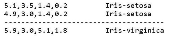
Figure 1. Examples of patterns included in the iris.data file.

However, the algorithmic steps of the linear associator require column patterns, both for the input and output. Therefore, when implementing the algorithm, each of the row patterns is simply taken and converted into a column pattern as in Equation (15), thus avoiding unnecessary excess notation.

Below is an example of an Iris versicolor class pattern and the corresponding class labels for patterns 51 through 100:

$$x^{51}=\left(\begin{array}{c}7.0\\ 3.2\\ 4.7\\ 1.4\end{array}\right)\in {ℝ}^4$$

(18)

$$y^{51}=2;y^{52}=2;\cdots ;y^{100}=2$$

(19)

Similarly, the class pattern is as follows for the class Iris virginica:

$$x^{101}=\left(\begin{array}{c}6.3\\ 3.3\\ 6.0\\ 2.5\end{array}\right)\in {ℝ}^4$$

(20)

$$y^{101}=3;y^{102}=3;\cdots ;y^{150}=3$$

(21)

As in any pattern classification experiment, the first thing to do is choose a validation method. For this example, leave-one-out [16] has been selected. Therefore, the first pattern of class 1, $x^1$, is chosen as the test pattern, while all the remaining 149 patterns constitute the training set.

The training phase of the linear associator is started by applying Equation (3) to the first pattern of the training set, which is $x^2$, and whose class label is $y^2$:

$$y^2·{\left(x^2\right)}^t=\left(1\right)·{\left(\begin{array}{c}4.9\\ 3.0\\ 1.4\\ 0.2\end{array}\right)}^t=\left(1\right)·\left(4.93.01.40.2\right)=\left(4.93.01.40.2\right)$$

(22)

The same process is carried out with the following association, which is $\left(x^3,y^3\right)$:

$$y^3·{\left(x^3\right)}^t=\left(1\right)·{\left(\begin{array}{c}4.7\\ 3.2\\ 1.3\\ 0.2\end{array}\right)}^t=\left(1\right)·\left(4.73.21.30.2\right)=\left(4.73.21.30.2\right)$$

(23)

This continues until concluding with the 49 pattern associations of class 1. Then, the same process is applied to the first association of class 2, which is $\left(x^{51},y^{51}\right)$:

$$y^{51}·{\left(x^{51}\right)}^t=\left(2\right)·{\left(\begin{array}{c}7.0\\ 3.2\\ 4.7\\ 1.4\end{array}\right)}^t=\left(2\right)·\left(7.03.24.71.4\right)=\left(14.06.49.42.8\right)$$

(24)

This continues until concluding with the 50 pattern associations of class 2. Then, the same process is applied to the first association of class 3, which is $\left(x^{101},y^{101}\right)$:

$$y^{101}·{\left(x^{101}\right)}^t=\left(3\right)·{\left(\begin{array}{c}6.3\\ 3.3\\ 6.0\\ 2.5\end{array}\right)}^t=\left(3\right)·\left(6.33.36.02.5\right)=\left(18.99.918.07.5\right)$$

(25)

This process continues until the last association is reached, which is $\left(x^{150},y^{150}\right)$. At the end, there are 149 matrices of dimensions $1\times 4$, which are added according to Equation (4) to finally obtain the linear associator. The matrix M representing the linear associator is also of dimensions $1\times 4$:

$$M^{\left(1\right)}=\left(1827.0890.51330.6448.5\right)$$

(26)

The symbol (1) as a superscript in $M^{\left(1\right)}$ indicates that the pattern $x^1$, being the test pattern, has not participated in the learning phase.

Now that the linear associator $M^{\left(1\right)}$ has been trained, it is time to move on to the classification phase. For this, Equation (6) is applied to linear associator $M^{\left(1\right)}$ in Equation (26) and to the test pattern $x^1$ in Equation (15):

$$M^{\left(1\right)}·x^1=\left(1827.0890.51330.6448.5\right)·\left(\begin{array}{c}5.1\\ 3.5\\ 1.4\\ 0.2\end{array}\right)=14387$$

(27)

The returned value in Equation (27), 14,281, is a long way from the expected value, which is the class label $y^1=1$. This is because the 149 patterns the linear associator trains with are far from orthonormal, as is required by the original linear associator model for pattern recalling to be correct (Theorem 1).

This is where one of the original contributions of this paper comes into play. By applying this idea, it is possible to solve the problem of obtaining a number that is very far from the class label. By applying a scaling and a rounding, it is possible to bring the result closer to the class label of the test pattern $x^1$:

$$M^{\left(1\right)}·x^1=14,387\to round\left(\frac{14,387}{10,000}\right)=round\left(1.4387\right)=1=y^1$$

(28)

The class label for test pattern $x^1$ was successfully recalled. It was a hit of the classifier, but what will happen to the other patterns in the dataset?

To find out, let us go to the second iteration of the leave-one-out validation method, where the pattern $x^2$ will now become a test pattern, while the training set will be formed with the 149 remaining patterns from the dataset, which are

$$x^1,x^3,x^4,\cdots ,x^{150}$$

(29)

When executing steps similar to those of iteration 1 based on Equations (3) and (4), the linear associator is obtained:

$$M^{\left(2\right)}=\left(1827.2891.01330.6448.5\right)$$

(30)

Again, the symbol (2) as a superscript in $M^{\left(2\right)}$ indicates that the pattern $x^2$, being the test pattern, has not participated in the learning phase. Now that the linear associator $M^{\left(2\right)}$ has been trained, it is time to move on to the classification phase. For this, Equation (6) is applied to linear associator $M^{\left(2\right)}$ in Equation (30) and to the test pattern $x^2$ in Equation (15):

$$M^{\left(2\right)}·x^2=\left(1827.2891.01330.6448.5\right)·\left(\begin{array}{c}4.9\\ 3.0\\ 1.4\\ 0.2\end{array}\right)=13579$$

(31)

Again, by applying a scaling and a rounding, it is possible to bring the result closer to the class label of the test pattern $x^2$:

$$M^{\left(2\right)}·x^2=13579\to round\left(\frac{13579}{10000}\right)=round\left(1.3579\right)=1=y^2$$

(32)

Something similar happens when executing iterations 3, 4 and 5, where the class labels of the test patterns $x^3,x^4$, and $x^5$ are correctly recalled. However, it is interesting to observe what happens in iteration 6, where the test pattern is now $x^6$:

$$M^{\left(6\right)}=\left(1826.7890.11330.3448.3\right)$$

(33)

$$M^{\left(6\right)}·x^6=\left(1826.7890.11330.3448.3\right)·\left(\begin{array}{c}5.4\\ 3.9\\ 1.7\\ 0.4\end{array}\right)=15776$$

(34)

$$M^{\left(6\right)}·x^6=15,776\to round\left(\frac{15,776}{10,000}\right)=round\left(1.5776\right)=2\ne y^6$$

(35)

This is a classifier error, because the result should be label 1, while the linear associator assigns label 2 to the test pattern $x^6$. However, this is not the only mistake. The total number of patterns in class 1 (Iris setosa) that are mislabeled is 12.

Now, it is the turn of iteration 51, which corresponds to the first test pattern of class 2 (Iris versicolor). When executing steps similar to those of iteration 1, based on Equations (3) and (4), the linear associator is obtained:

$$M^{\left(51\right)}=\left(1818.1887.61322.6445.9\right)$$

(36)

$$M^{\left(51\right)}·x^{51}=\left(1818.1887.61322.6445.9\right)·\left(\begin{array}{c}7.0\\ 3.2\\ 4.7\\ 1.4\end{array}\right)=22407$$

(37)

$$M^{\left(51\right)}·x^{51}=22,407\to round\left(\frac{22,407}{10,000}\right)=round\left(2.2407\right)=2=y^{51}$$

(38)

This is a hit of the classifier, because the linear associator correctly assigns label 2 to the test pattern $x^{51}$. The same happens with all 50 patterns of class 2. There are zero errors in this class.

Now, it is the turn of iteration 101, which corresponds to the first test pattern of class 3 (Iris virginica). When executing steps similar to those of iteration 1, based on Equations (3) and (4), the linear associator is obtained:

$$M^{\left(101\right)}=\left(1813.2884.11314.0441.2\right)$$

(39)

$$M^{\left(101\right)}·x^{101}=\left(1813.2884.11314.0441.2\right)·\left(\begin{array}{c}6.3\\ 3.3\\ 6.0\\ 2.5\end{array}\right)=23328$$

(40)

$$M^{\left(101\right)}·x^{101}=23,328\to round\left(\frac{23,328}{10,000}\right)=round\left(2.3328\right)=2\ne y^{101}$$

(41)

This is a classifier error, because test pattern $x^{101}$ belongs to class 3. There are 43 errors in this class, and only 7 of the 50 patterns in class 3 (Iris virginica) are correctly classified by the linear associator.

The sum of all the errors of the linear associator in the Iris Dataset is 55. That is, the Linear Associator acting as a pattern classifier on the Iris Dataset obtains 95 total hits. Since the Iris Dataset is balanced, it is possible to use accuracy as a good performance measure [16]:

$$Accuracy=\left(\frac{Numberofhits}{Totaltestedpatterns}\right)·\left(100\right)=\left(\frac{95}{150}\right)·\left(100\right)=63.33\%$$

(42)

How good or bad is this performance? A good way to find out is to compare the accuracy obtained by the linear associator with the performances exhibited by the classifiers of the state of the art.

For this, seven of the most important classifiers of the state of the art have been selected, which will be detailed in Section 4.2: a Bayesian classifier (Naïve Bayes [19]), two algorithms of the nearest neighbors family (1-NN and 3-NN [20]), a decision tree (C4.5 [21]), a support vector machine (SVM [22]), a neural network (MLP [23]), and an ensemble of classifiers (random forest [24]).

In all cases, the same validation method has been used: leave-one-out. Table 1 contains the accuracy values (best in bold), where LA stands for linear associator.

Table 1. Accuracy values (as percentages) exhibited by the state-of-the-art classifiers in the Iris Dataset.

	Naïve Bayes	1-NN	3-NN	C4.5	SVM	MLP	Random Forest	LA
Iris Dataset	95.33	95.33	95.33	95.33	96.00	96.66	94.66	63.33

The accuracy obtained by the linear associator is more than thirty percentage points below the performance exhibited by the seven most important classifiers of the state of the art for different approaches.

This means that if the linear associator is to be converted into a competitive classifier, at least in the Iris Dataset, it is necessary to improve performance by thirty or more percentage points when accuracy is used as a performance measure.

That is not easy at all.

In Section 2.1, it was pointed out that, based on the known results of elementary linear algebra, it happens to be that, in general, for a set of input vectors of the linear associator of $n$ compents, in a set of $n+1$ vectors or greater, it will no longer be possible to make all vectors orthonormal. This means, among other things, that it is not possible to orthonormalize the 150 patterns of 4 attributes of the Iris Dataset.

The central and most relevant proposal of this paper is to improve the performance of the linear associator through a transformation of the patterns. That transformation is achieved through a powerful mathematical tool called singular value decomposition.

2.3. Singular Value Decomposition (SVD)

Given a matrix $A\in {ℝ}^{m\times n}$ where $m,n$ are positive integral numbers, it is possible to represent that matrix using the singular value decomposition (SVD) [14] as in Equation (43):

$$A=US{V}^T$$

(43)

where $U\in {ℝ}^{m\times m}$ and $V\in {ℝ}^{n\times n}$ are orthonormal matrices with respect to the columns. In addition, $S\in {ℝ}^{m\times n}$ is a non-negative matrix diagonal containing the square roots of the eigenvalues (which are called singular values) from $U$ or $V$ in descending order and the zeros off the diagonal.

If $m>n$, it is possible to establish the equality $S=\left[\begin{array}{c}\widehat{S}\\ 0\end{array}\right]$.

Therefore, matrix A in Equation (43) can be represented by the “economy SVD” [15]:

$$A=US{V}^T=\left[\begin{array}{cc}\widehat{U}& {\widehat{U}}^{\perp }\end{array}\right]\left[\begin{array}{c}\widehat{S}\\ 0\end{array}\right]V^T=\widehat{U}\widehat{S}{V}^T$$

(44)

where ${\widehat{U}}^{\perp }$ contains the columns that make up a complementary vector space orthogonal to $\widehat{U}$. Note that matrix $\widehat{U}$ has the same dimensions as matrix $A$. In Figure 2, the economy SVD is schematized.

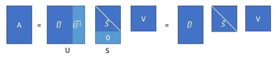
Figure 2. Schematic representation of the economy SVD from Equation (44).

The process followed to obtain the SVD from matrix $A$ in Equation (45) is exemplified below:

$$A=\left[\begin{array}{cc}-2& 4\\ 5& 0\\ -2& -1\end{array}\right]$$

(45)

The first step is to find $A^T$ in Equation (46) and then calculate $A{A}^T$ in Equation (47):

$$A^T=\left[\begin{array}{ccc}-2& 5& -2\\ 4& 0& -1\end{array}\right]$$

(46)

$$A{A}^T=\left[\begin{array}{cc}-2& 4\\ 5& 0\\ -2& -1\end{array}\right]\left[\begin{array}{ccc}-2& 5& -2\\ 4& 0& -1\end{array}\right]=\left[\begin{array}{ccc}20& -10& 0\\ -10& 25& -10\\ 0& -10& 5\end{array}\right]$$

(47)

Next, we need to find the eigenvectors of $A{A}^T$ and their corresponding eigenvalues. Therefore, we will use Equation (48), which defines the eigenvectors of the matrix $A{A}^T$:

$$\left[\begin{array}{ccc}20& -10& 0\\ -10& 25& -10\\ 0& -10& 5\end{array}\right]\left[\begin{array}{c}{x}_1\\ x_2\\ x_3\end{array}\right]=\mathsf{\lambda }\left[\begin{array}{c}{x}_1\\ x_2\\ x_3\end{array}\right]$$

(48)

From Equation (48), we obtain the system of equations shown in Equation (49):

$$\begin{gathered} (20-\mathsf{\lambda })x_1-10x_2=0 \\ -10x_1+\left(25-\mathsf{\lambda }\right)x_2-10x_3=0 \\ -10x_2+\left(5-\mathsf{\lambda }\right)x_3=0 \end{gathered}$$

(49)

Solving for $\mathsf{\lambda }$ by the method of minors in Equation (50) yields

$$\left|\begin{array}{ccc}20-\mathsf{\lambda }& -10& 0\\ -10& 25-\mathsf{\lambda }& -10\\ 0& -10& 5-\mathsf{\lambda }\end{array}\right|=0$$

(50)

Therefore, the eigenvalues of $A{A}^T$ are

$$\lambda =0,\lambda =15,\lambda =35$$

(51)

To obtain the eigenvector of $\lambda =35$, the system in Equation (49) is used:

$$\begin{gathered} x_1-2x_3=0 \\ {x}_2+3x_3=0 \end{gathered}$$

Consequently, the eigenvector for the eigenvalue $\lambda =35$ is

$$\overrightarrow{{\nu }_1}=\left[\begin{array}{ccc}2& -3& 1\end{array}\right]$$

(52)

The corresponding expressions to find the eigenvectors of the remaining eigenvalues $\lambda =15$ and $\lambda =0$ are

$$\begin{gathered} x_1+2x_3=0 \\ {x}_2+x_3=0 \end{gathered}$$

$$\overrightarrow{{\nu }_2}=\left[\begin{array}{ccc}-2& -1& 1\end{array}\right]$$

(53)

$$\begin{gathered} 4x_1-x_3=0 \\ 2x_2-x_3=0 \end{gathered}$$

$$\overrightarrow{{\nu }_3}=\left[\begin{array}{ccc}1& 2& 4\end{array}\right]$$

(54)

When ordering the eigenvectors $\overrightarrow{{\nu }_1}$,$\overrightarrow{{\nu }_2}$, and $\overrightarrow{{\nu }_3}$ with Equations (52)–(54) as columns of a matrix, we obtain

$$\left[\begin{array}{ccc}2& -2& 1\\ -3& -1& 2\\ 1& 1& 4\end{array}\right]$$

(55)

By normalization of Equation (55), the matrix $U$ is obtained [17]:

$$U=\left[\begin{array}{ccc}\frac{-2}{\sqrt{14}}& \frac{-2}{\sqrt{6}}& \frac{1}{\sqrt{21}}\\ \frac{3}{\sqrt{14}}& \frac{-1}{\sqrt{6}}& \frac{2}{\sqrt{21}}\\ \frac{-1}{\sqrt{14}}& \frac{-1}{\sqrt{6}}& \frac{4}{\sqrt{21}}\end{array}\right]$$

(56)

The calculation of $V$ is similar, but this time, it will be based on the matrix $A^{T}A$, which is calculated in Equation (57), from the matrices $A^T$ in Equation (46) and $A$ in Equation (45):

$$A^{T}A=\left[\begin{array}{ccc}-2& 5& -2\\ 4& 0& -1\end{array}\right]\left[\begin{array}{cc}-2& 4\\ 5& 0\\ -2& -1\end{array}\right]=\left[\begin{array}{cc}33& -6\\ -6& 17\end{array}\right]$$

(57)

After executing the algorithmic steps corresponding to those performed in Equations (48)–(54), this matrix is obtained:

$$\left[\begin{array}{cc}3& -1\\ -1& -3\end{array}\right]$$

(58)

By normalization of Equation (58), the matrix $V$ is obtained [17]:

$$V=\left[\begin{array}{cc}\frac{3}{\sqrt{10}}& \frac{-1}{\sqrt{10}}\\ \frac{-1}{\sqrt{10}}& \frac{-3}{\sqrt{10}}\end{array}\right]$$

(59)

The matrix $S$ is built from a matrix full of zeros of dimensions $m\times n$. Then, the zeros of the diagonal are replaced with the singular values (which are the square roots of the eigenvalues) of matrix $U$ in descending order.

In our example, the singular values of the matrix $U$ are obtained with the square root of the first two eigenvalues in Equation (51):

$$S=\left[\begin{array}{cc}\sqrt{35}& 0\\ 0& \sqrt{15}\\ 0& 0\end{array}\right]$$

(60)

Therefore, according to Equation (43), the SVD of matrix A is expressed as in Equation (61):

$$A=US{V}^T=\left[\begin{array}{ccc}\frac{-2}{\sqrt{14}}& \frac{-2}{\sqrt{6}}& \frac{1}{\sqrt{21}}\\ \frac{3}{\sqrt{14}}& \frac{-1}{\sqrt{6}}& \frac{2}{\sqrt{21}}\\ \frac{-1}{\sqrt{14}}& \frac{-1}{\sqrt{6}}& \frac{4}{\sqrt{21}}\end{array}\right]\left[\begin{array}{cc}\sqrt{35}& 0\\ 0& \sqrt{15}\\ 0& 0\end{array}\right]{\left[\begin{array}{cc}\frac{3}{\sqrt{10}}& \frac{-1}{\sqrt{10}}\\ \frac{-1}{\sqrt{10}}& \frac{-3}{\sqrt{10}}\end{array}\right]}^T$$

(61)

Now, from Equation (60), it is possible to obtain the matrix $\widehat{S}$:

$$\widehat{S}=\left[\begin{array}{cc}\sqrt{35}& 0\\ 0& \sqrt{15}\end{array}\right]$$

(62)

Finally, according to Equation (44), the economy SVD of matrix A is expressed as in Equation (63):

$$A=\widehat{U}\widehat{S}{V}^T=\left[\begin{array}{cc}\frac{-2}{\sqrt{14}}& \frac{-2}{\sqrt{6}}\\ \frac{3}{\sqrt{14}}& \frac{-1}{\sqrt{6}}\\ \frac{-1}{\sqrt{14}}& \frac{-1}{\sqrt{6}}\end{array}\right]\left[\begin{array}{cc}\sqrt{35}& 0\\ 0& \sqrt{15}\end{array}\right]{\left[\begin{array}{cc}\frac{3}{\sqrt{10}}& \frac{-1}{\sqrt{10}}\\ \frac{-1}{\sqrt{10}}& \frac{-3}{\sqrt{10}}\end{array}\right]}^T$$

(63)

The matrices $\widehat{S}$ and $V^T$ in Equations (44) and (63) have something in common. For both matrices, the inverse matrix is defined, and its calculation is extremely simple [15]. The importance of this property for this paper will be evident in Section 3, where the proposed methodology is described.

The inverse matrix of V is calculated as follows:

$${\left(V^T\right)}^{-1}={\left(V^T\right)}^T=V$$

(64)

On the other hand, let $\widehat{S}$ be of dimensions $n\times n$, whose elements on its diagonal are $s_{11},s_{22},\cdots ,s_{nn}$. Then, the inverse matrix of $\widehat{S}$ is calculated as follows:

$${\left(\widehat{S}\right)}^{-1}=\left(\begin{array}{ccc}\frac{1}{s_{11}}& \cdots & 0\\ ⋮& \ddots & ⋮\\ 0& \cdots & \frac{1}{s_{nn}}\end{array}\right)$$

(65)

It can be easily verified that Equations (64) and (65) are fulfilled in the matrices of Equation (63).

An interesting application of Equations (64) and (65) is that it is possible to express the matrix $\widehat{U}$ in Equation (44) as a function of $\widehat{S}$ and $V$:

$$A=\widehat{U}\widehat{S}{V}^T$$

$$\left(A\right){\left(V^T\right)}^{-1}=\left(\widehat{U}\widehat{S}{V}^T\right){\left(V^T\right)}^{-1}$$

$$\left(A\right){\left(V^T\right)}^{-1}=\left(\widehat{U}\widehat{S}\right)\left[\left(V^T\right){\left(V^T\right)}^{-1}\right]$$

$$\left(A\right){\left(V^T\right)}^{-1}=\widehat{U}\widehat{S}$$

$$\left(A\right){\left(V^T\right)}^{-1}{\left(\widehat{S}\right)}^{-1}=\left(\widehat{U}\right)\left[\left(\widehat{S}\right){\left(\widehat{S}\right)}^{-1}\right]$$

$$\left(A\right){\left(V^T\right)}^{-1}{\left(\widehat{S}\right)}^{-1}=\widehat{U}$$

$$\widehat{U}=AV{\left(\widehat{S}\right)}^{-1}$$

(66)

It is possible to interpret Equation (66) in an unorthodox way. This novel interpretation gives rise to one of the original contributions of this paper.

If the matrices $A$, $V$, and $\widehat{S}$ are known, it is possible to interpret Equation (66) as the generation of the matrix $\widehat{U}$ by transforming the data in $A$ through the modulation of these data by the $V{\left(\widehat{S}\right)}^{-1}$ product.

However, there is something else of great relevance for the original proposal of this paper, which will be explained in Section 3. It is possible to set a vector as $A$ so that $\widehat{U}$ will be a vector transformed in the same way as matrix $\widehat{U}$ in Equation (66).

3. Our Proposal

It is assumed that a dataset $D$ is available which is designed for the classification task in machine learning. As such, the dataset consists of $p$ associations of patterns whose components are real numbers as in Equation (1). As was the case before, $p$ is a positive integer indicating the cardinality of the dataset:

$$D=\left\{\left(x^{\mu },y^{\mu }\right)|\mu =1,2,\dots ,p\right\}$$

(67)

However, in this special $D$, there is something new. While the first element of each association is an input pattern of dimension $n$ (as before, $n$ is a positive integer indicating the dimension of the input patterns), the second element of each association is the corresponding output pattern of dimension $m=1$. The novelty occurs in this second element of each association, because each output pattern represents the encoding of the corresponding class label of the input pattern $\left(1,2,3,\cdots \right)$. It is also assumed that the number of classes is less than 10.

Therefore, Equation (2) for $D$ is modified as follows:

$$x^{\mu }={\left(x_1^{\mu },x_2^{\mu },\dots ,x_n^{\mu }\right)}^t=\left(\begin{array}{c}{x}_1^{\mu }\\ x_1^{\mu }\\ ⋮\\ x_n^{\mu }\end{array}\right)\in {ℝ}^n;y^{\mu }\in {\mathbb{Z}}^{+}\subset ℝ$$

(68)

When implementing the algorithm of this proposal, each input pattern is considered a column vector.

It is also assumed that a validation method is applied. The result of applying the validation method is a partition of the dataset $D$ into two disjoint subsets: a training or learning set $L$ and a test set $T$, which will change with each iteration of the algorithm. The number of iterations that the algorithm performs is directly determined by the choice of the validation method to be applied.

At each iteration, it is possible to explicitly identify the conformation of the sets $L$ and $T$. If the cardinality of the training or learning set $L$ is $l$, then $l<p$, and $L$ is made up of two sets of different natures but with the same cardinality $l$. On the one hand, there exists the set of training or learning patterns $X_L$, which contains $l$ patterns of $n$ real components each. On the other hand, $L$ also contains a set $Y_L$, which is an ordered list of the corresponding labels that are elements of $X_L$. In the training or learning phase of the new algorithm, both sets $X_L$ and $Y_L$ are actively involved.

Something similar happens with the test set $T$, which will have a cardinality equal to $p-l$. The test set $T$ is made up of two sets of different natures but with the same cardinality $p-l$. On the one hand, there exists the set of test patterns $X_T$, which contains $p-l$ patterns of $n$ real components each. On the other hand, $T$ also contains a set $Y_T$, which is an ordered list of the corresponding labels of that are elements of $X_T$. In the classification phase of the new algorithm, only the patterns of the $X_T$ set are involved, and the algorithm itself will respond with the class labels. Since the proposed algorithm belongs to the supervised paradigm, the set $Y_T$ will only be used by the practitioner, who must verify if the algorithm had success or an error when classifying a specific pattern extracted from the set $X_T$. The labels of the set $Y_T$ are never known by the algorithm.

Without loss of generality, it is possible to assume that the well-known K-fold cross-validation method is chosen [16]. In this paper, we use the value $K=10$.

The rest of this section contains three subsections. Section 3.1 and Section 3.2 describe the training or learning phase and the classification phase of the proposed algorithm, respectively. Both sections include original proposals that ostensibly enrich the performance of the linear associator as a pattern classifier. Due to the important role that SVD plays in the design and implementation of the proposed algorithm, we have called the new algorithm the linear associator with singular value decomposition (LA-SVD).

Section 3.3 is relevant because it exemplifies the benefits of the proposed algorithm. The same example of Section 2.2 is carried out with the new algorithm, and the results are compared, which show the superiority of the LA-SVD algorithm.

3.1. LA-SVD Training or Learning Phase

To start the training or learning phase, first, the $X_L$ set is transformed using the economy SVD into a new transformed $\widehat{X_L}$ set. Then, the algorithmic steps of the training or learning phase of the original linear associator are applied.

3.1.1 In Equation (44), replace $\mathrm{A}$ with ${\mathrm{X}}_{\mathrm{L}}$:

$$X_L=\widehat{U}\widehat{S}{V}^T$$

(69)

3.1.2 In Equation (66), establish that $\widehat{U}$ is the transformed set $\widehat{X_L}$:

$$\widehat{X_L}=X_{L}V{\left(\widehat{S}\right)}^{-1}$$

(70)

This step is really disruptive because a new set of training or learning has been obtained through the modulation of $X_L$ by the $V{\left(\widehat{S}\right)}^{-1}$ product. Note that both sets $X_L$ and $\widehat{X_L}$ have the same cardinality $l$. Note also that the set of class labels $Y_L$ remains unchanged.

3.1.3 Each transformed training column pattern ${\left(\widehat{x_L}\right)}^{\mu }$ is operated with its corresponding class label $y^{\mu }$, $\mu \in \left\{1,2,\cdots ,l\right\}$ to form the $\mathsf{\mu }$-th matrix of dimensions $1\times \mathrm{n}$:

$$y^{\mu }·{\left[{\left(\widehat{x_L}\right)}^{\mu }\right]}^t=y^{\mu }·\left[{\left(\widehat{x_L}\right)}_1^{\mu }{\left(\widehat{x_L}\right)}_2^{\mu }\cdots {\left(\widehat{x_L}\right)}_n^{\mu }\right]=\left[y^{\mu }·{\left(\widehat{x_L}\right)}_1^{\mu }{y}^{\mu }·{\left(\widehat{x_L}\right)}_2^{\mu }\cdots y^{\mu }·{\left(\widehat{x_L}\right)}_n^{\mu }\right]$$

(71)

3.1.4 The $l$ $\mu$-th matrices are added to form the matrix $\widehat{M}$ of dimensions 1 × n:

$$\widehat{M}={\displaystyle \sum }_{\mu =1}^l{y}^{\mu }·{\left[{\left(\widehat{x_L}\right)}^{\mu }\right]}^t$$

(72)

This obtained matrix $\widehat{M}$ is precisely the already trained LA-SVD.

For each iteration, which is determined by the validation method, steps 3.1.1–3.1.4 are repeated.

3.2. LA-SVD Classification Phase

In this phase, the already trained LA-SVD will be matrix-operated with a test pattern, and a class label will be predicted. Subsequently, the practitioner will contrast the result given by the LA-SVD with the real class label and will use that information to determine the performance of the new algorithm. Two disruptive original ideas are important parts in this LA-SVD classification phase.

In a specific iteration where the training or learning phase has been carried out with the set $X_L$, a test pattern ${\left(x_T\right)}^{test}$ is selected from the test set $X_T$. Note that the label of this test pattern is unknown by the algorithm, because neither this pattern nor its label intervene in the training phase.

3.2.1 The first disruptive original idea of this subsection consists of making the decision that the test pattern ${\left(x_T\right)}^{test}$ must be transformed in the same way that the training or learning set $X_L$ was transformed into $\widehat{X_L}$ by Equation (70):

$${\left(\widehat{x_T}\right)}^{test}={\left(x_T\right)}^{test}V{\left(\widehat{S}\right)}^{-1}$$

(73)

3.2.2 The product between the matrix $\widehat{M}$ in Equation (72) is performed with the transformed testing column pattern ${\left(\widehat{x_T}\right)}^{test}$:

$$\widehat{M}·{\left(\widehat{x_T}\right)}^{test}=\left[{\widehat{M}}_1{\widehat{M}}_2\cdots {\widehat{M}}_n\right]·\left[\begin{array}{c}{\left(\widehat{x_T}\right)}_1^{test}\\ \begin{array}{c}{\left(\widehat{x_T}\right)}_2^{test}\\ ⋮\end{array}\\ {\left(\widehat{x_T}\right)}_n^{test}\end{array}\right]=r\in ℝ$$

(74)

3.2.3 This step contains the second disruptive original idea of this subsection. The result of the previous step is a number $r\in ℝ$ that is not necessarily a class label, which is typically represented by a small positive integer, as was discussed earlier in this paper. Therefore, the label predicted by the classifier is obtained by rounding the real number $r$ to the nearest positive integer:

$${\left(\widehat{y}\right)}^{test}=round\left(r\right)$$

(75)

The value ${\left(\widehat{y}\right)}^{test}$ is a positive integer less than 10, and it is expected to correspond with the true class label of the test pattern ${\left(x_T\right)}^{test}$.

3.3. Illustrative Example

In this subsection, the example developed and detailed in Section 2.2, where the linear associator was applied to the Iris Dataset, will be replicated. This time, the new LA-SVD algorithm will be applied to the same dataset, and the results will be compared.

It should be emphasized that the Iris Dataset meets the previously specified assumption, because in this dataset, the number of classes is 3 (i.e., less than 10).

As in the example in Section 2.2, leave-one-out has been selected as the validation method. The first pattern of class 1 is chosen as the test pattern so that ${\left(x_T\right)}^{test}=x^1$, while all the remaining 149 patterns constitute the training or learning set $X_L$.

For this first iteration, the matrices $\widehat{S}$ and $V^T$ are

$$\widehat{S}=\left[\begin{array}{cccc}95.7685& 0& 0& 0\\ 0& 17.5720& 0& 0\\ 0& 0& 3.4693& 0\\ 0& 0& 0& 1.8789\end{array}\right]$$

(76)

$$V^T=\left[\begin{array}{cccc}-0.7507& 0.2870& 0.4994& 0.3235\\ -0.3790& 0.5455& -0.6750& -0.3212\\ -0.5142& -0.7081& -0.0547& -0.4808\\ -0.1684& -0.3445& -0.5403& 0.7490\end{array}\right]$$

(77)

From here, Equations (64) and (65) are used to get the inverse matrices ${\left(V^T\right)}^{-1}$ and ${\left(\widehat{S}\right)}^{-1}$:

$${\left(V^T\right)}^{-1}=V=\left[\begin{array}{cccc}-0.7507& -0.3790& -0.5142& -0.1684\\ 0.2870& 0.5455& -0.7081& -0.3445\\ 0.4994& -0.6750& -0.0547& -0.5403\\ 0.3235& -0.3212& -0.4808& 0.7490\end{array}\right]$$

(78)

$${\left(\widehat{S}\right)}^{-1}=\left[\begin{array}{cccc}0.0104& 0& 0& 0\\ 0& 0.0569& 0& 0\\ 0& 0& 0.2882& 0\\ 0& 0& 0& 0.5322\end{array}\right]$$

(79)

Applying Equation (70) results in the transformed set $\widehat{X_L}$, whose first pattern is the transformed pattern of $x^2$:

$${\left(\widehat{x_L}\right)}^2=\left(\begin{array}{c}-0.0582\\ 0.1128\\ 0.0684\\ 0.0521\end{array}\right)\in {ℝ}^4$$

(80)

By applying Equation (71), we get

$$y^2·{\left[{\left(\widehat{x_L}\right)}^2\right]}^t=\left[-0.05820.11280.06840.0521\right]$$

(81)

In addition, after calculating and adding the 149 matrices, by Equation (72), we get

$${\widehat{M}}^{\left(1\right)}=\left[-25.7790-4.9314-1.09440.5880\right]$$

(82)

According to Equation (15), the test pattern is

$${\left(x_T\right)}^{test}=x^1=\left(\begin{array}{c}5.1\\ 3.5\\ 1.4\\ 0.2\end{array}\right)\in {ℝ}^4$$

(83)

By applying Equations (73), (78), (79), and (83), we get

$${\left(\widehat{x_T}\right)}^{test}={\left(x_T\right)}^{test}V{\left(\widehat{S}\right)}^{-1}=\left(\begin{array}{c}-0.0617\\ 0.1316\\ -0.0001\\ 0.0011\end{array}\right)$$

(84)

By applying Equations (74), (82), and (84), we get

$${\widehat{M}}^{\left(1\right)}·{\left(\widehat{x_T}\right)}^{test}=\left[-25.7790-4.9314-1.09440.5880\right]·\left[\begin{array}{c}-0.0617\\ 0.1316\\ -0.0001\\ 0.0011\end{array}\right]=0.9422$$

(85)

By applying the rounding specified in Equation (75) to the real number obtained in Equation (85), the label predicted by the LA-SVD classifier is obtained:

$${\left(\widehat{y}\right)}^{test}=round\left(0.9422\right)=1$$

(86)

This is the label predicted by the LA-SVD classifier for the test pattern ${\left(x_T\right)}^{test}=x^1$. Note that this is a hit for the LA-SVD classifier because, in effect, the test pattern label is 1, since it belongs to the Iris setosa class.

When executing iterations 2, 3, 4 and 5, which correspond to the test patterns $x^2$, $x^3$, $x^4$, and $x^5$, the following values were obtained: 0.8972, 0.8763, 0.9049, and 0.9417. When the rounding specified in Equation (75) was applied to these four real numbers, in all cases, the label predicted by the LA-SVD classifier was 1, which matched the true labels.

Then comes iteration 6, in which the test pattern is $x^6$. The interest of this sixth iteration is that the linear associator erroneously predicts the corresponding label $y^6$. It is time to check how the LA-SVD behaves when it tries to classify test pattern $x^6$.

Since test pattern $x^6$ belongs to the class Iris setosa, it corresponds to label 1. However, according to Equation (35), the linear associator erroneously assigns label 2 to test pattern $x^6$. In contrast, the real number generated by applying Equation (74) was 1.1625, so rounding it using Equation (75) gave the correct label $y^6=1$.

When concluding with the classification of the 50 patterns of class 1, it is now possible to contrast the performances of both classifiers. While the linear associator classified 12 patterns incorrectly (12 errors), the new LA-SVD classifier exhibited zero errors; that is, all 50 patterns of the Iris setosa class were classified correctly.

After testing the 150 patterns of the Iris Dataset with the performance shown by the proposed LA-SVD, it was possible to compare these results with the classifiers in Table 1. While the linear associator returned 53 errors, the new classifier only made a mistake in the assignment of 6 labels. Knowing that there were only 6 errors, the accuracy value of the LA-SVD classifier was calculated with the 144 correct answers. For this, Equation (42) was used:

$$AccuracyofLA-SVDonIrisDataset=\left(\frac{144}{150}\right)·\left(100\right)=96\%$$

(87)

Table 2 contains the values of Table 1 updated with the accuracy result obtained by the LA-SVD classifier.

Table 2. Accuracy values updated with the result of the LA-SVD classifier.

	Naïve Bayes	1-NN	3-NN	C4.5	SVM	MLP	Random Forest	LA	LA-SVD
Iris Dataset	95.33	95.33	95.33	95.33	96.00	96.66	94.66	63.33	96.00

The results in Table 2 show the superiority of the proposed algorithm (LA-SVD) over the original linear associator, but on top of that, the LA-SVD is in second place in the comparison table against the best classifiers in the state of the art. By classifying the Iris Dataset, the LA-SVD classifier becomes a competitive classifier, because it improved the performance of the original linear associator by more than thirty percentage points when accuracy was used as a performance measure.

It is very important to clarify that this notable improvement in the results reported by the LA-SVD was not due to the orthonormality of the input patterns of the Iris Dataset. The explanation for this improvement in results lies in the fact that the benefits of orthonormality were taken advantage of in the columns of matrix $\widehat{U}$ in SVD.

Now is the time to take advantage of the benefits of the LA-SVD classifier by applying it to data that are very sensitive for humans because they are related to health: medical datasets.

4. Experimental Results

In order to achieve impact applications of the new classifier, fourteen datasets were selected whose data refer to a very sensitive topic for human societies: health. The LA-SVD classifier would be applied to fourteen medical datasets.

This section consists of three subsections. In Section 4.1, the datasets used to carry out the experiments are described. Section 4.2, for its part, contains descriptions of nine of the pattern classifiers of the most important approaches to the state of the art, including three classifier ensembles. The results obtained by these state-of-the-art algorithms are presented in Section 4.3, which also includes discussions and statistical comparative analyses. All of this will be of great support to measure the performance of the new algorithm proposed (LA-SVD) and the relevance that it will potentially acquire in the state of the art of machine learning and its applications.

4.1. Datasets

The fourteen medical datasets described had two classes and were balanced datasets. The balance or imbalance was determined by calculating the imbalance ratio ($IR$), which is an index that measures the degree of imbalance of a dataset. The $IR$ index was defined as in Equation (88):

$$IR=\frac{\left|majority\_class\right|}{\left|minority\_class\right|}$$

(88)

where $\left|majority\_class\right|$ represents the cardinality of the majority class in the dataset while $\left|minority\_class\right|$ represents the cardinality of the minority class.

A dataset was considered balanced if its $IR$ value was close to or less than 1.5 (note that the $IR$ value is always greater than 1).

To illustrate the concept of the $IR$ index, the Diabetic Retinopathy Debrecen Dataset would be taken as an example, which has 1151 patterns included into two classes. The majority class contains 611 patterns, while in the minority class, there are 540 patterns:

$$IR=\frac{611}{540}=1.13$$

(89)

Therefore, the Diabetic Retinopathy Debrecen Dataset is a balanced dataset.

Arcene Dataset [25]

This dataset was created by bringing together three cancer databases detected by mass spectrometry. It has 200 patterns and 10,000 attributes; the majority class has 112 patterns, and the minority class has 88 patterns. It has no missing values, and the $IR$ index is 1.27, which indicates that the dataset is balanced.

Bioresponse Dataset [25]

This dataset predicts a biological response of molecules from their chemical properties. It contains 3751 patterns and 1776 attributes. The majority class has 2034 patterns, and the minority class has 1717 patterns. It has no missing values. The $IR$ index is 1.18, which indicates that the dataset is balanced.

Breast Cancer Coimbra Dataset [18]

In the process of generating this dataset, breast cancer patients and healthy patients, which form the two classes, were examined. The dataset has 116 patterns and 9 attributes; the majority class has 64 patterns, and the minority class has 52 patterns. The dataset has no missing values, and the $IR$ index is 1.23, which indicates that the dataset is balanced.

Chronic Kidney Disease Dataset [18]

Its purpose is to diagnose if a patient has diabetes. It contains 400 patterns and 8 attributes. The majority class has 250 patterns, and the minority class has 150 patterns. It has missing values and categorical values in some attributes, so it was necessary to apply imputation to those missing values and label coding to the categorical values. The $IR$ index is 1.6, which indicates that this dataset is (almost) balanced.

Diabetic Retinopathy Debrecen Dataset [18]

This dataset contains data that allows knowing if a patient suffers from diabetic retinopathy. The dataset contains 1151 patterns and 19 attributes. The majority class has 611 patterns, and the minority class has 540 patterns. It has no missing values, and the $IR$ index is 1.13, which indicates that it is a balanced dataset.

Heart Attack Possibility Dataset [26]

This dataset contains 303 patterns and 14 attributes. The majority class has 165 patterns, and the minority class has 138 patterns. It has no missing values. The $IR$ index is 1.19, which indicates that the dataset is balanced.

Hungarian Heart Dataset [25]

This dataset contains 294 patterns and 14 attributes. The majority class has 188 patterns, and the minority class has 106 patterns. It has missing values and categorical data in some features, so it was necessary apply imputation to those missing values, and label coding was applied to the categorical values. The $IR$ index is 1.7, which indicates that the dataset is (almost) balanced.

Lymphography Dataset [25]

This dataset contains 148 patterns and 18 attributes. The majority class has 81 patterns, and the minority class has 67 patterns. It has no missing values, but it does have categorical values, so label coding was applied to these values. The $IR$ index is 1.2, which indicates that the dataset is balanced.

Pima Indians Diabetes Dataset [27]

Its purpose is to diagnose if a patient has diabetes. It contains 768 patterns and 8 attributes. The majority class has 500 patrons, and the minority class has 268. It has no missing values. The $IR$ index is 1.8, which indicates that the dataset is slightly imbalanced.

Plasma Retinol Dataset [25]

This dataset contains 315 patterns and 13 attributes. The majority class has 182 patterns, and the minority class has 133 patterns. It has no missing values, but it does have categorical values, so label coding was applied to these values. The $IR$ is 1.36, which indicates that the dataset is balanced.

Prnn Crabs Dataset [25]

This dataset contains 200 patterns and 7 attributes. The majority class has 100 patterns, and the minority class has 100 patterns. It has no missing values. The $IR$ index is 1, which indicates that the dataset is perfectly balanced.

South African Heart Disease Dataset [28]

This dataset was created through a study of men from the Western Cape in South Africa, where there is a high rate of death from coronary heart disease (CHD). The dataset is divided into those men who died from CHD and those men who responded to a treatment applied to them. It is worth mentioning that this database is only a fraction of the original database described in [29]. The dataset has 462 patterns and 10 attributes. The majority class has 302 patterns, and the minority class has 160 patterns. It has no missing values, and the $IR$ index is 1.8, which indicates that the dataset is slightly imbalanced. It has no missing values, but it does present mixed attributes, so the categorical attributes were changed to numerical ones.

Statlog Heart Dataset [18]

This dataset has 270 patterns and 13 attributes. The majority class has 150 patterns, and the minority class has 120 patterns. It has no missing values, and the $IR$ index is 1.15, which indicates that the dataset is balanced.

Tumors C Dataset [25]

This dataset was created to study patients with medulloblastomas. Medulloblastoma patients were treated and divided into two classes: medulloblastoma survivors (39 patterns) and those whose treatments failed (21 patterns). It has no missing values, and the $IR$ index is 1.8, which indicates that the dataset is slightly imbalanced.

Table 3 contains a summary of the specifications for the fourteen datasets.

Table 3. Description of the datasets in alphabetical order.

Dataset	Number of Patterns	Number of Features
Arcene	200	10,000
Bioresponse	3751	1776
Breast Cancer Coimbra	116	9
Chronic Kidney Disease	400	8
Diabetic Retinopathy Debrecen	1151	19
Heart Attack Possibility	303	14
Hungarian Heart	294	14
Lymphography	148	18
Pima Indians Diabetes	768	8
Plasma Retinol	315	13
Prnn Crabs	200	7
South African Heart Disease	462	10
Statlog Heart	270	13
Tumors C	60	7130

4.2. State-of-the-Art Classifiers for Comparison

This subsection describes the conceptual basis of nine of the most important classifiers of the state of the art (six of them are simple classifiers, and the other three are classifier ensembles) which were implemented on the WEKA platform [30]. These are the classification algorithms against which our proposal, the LA-SVD classifier, will be compared.

Simple Classifiers

Naïve Bayes [19,30]

The Naïve Bayes classifier is a probabilistic algorithm with a superstructure based on Bayes’ theorem. The classifier assumes that the features are independent of each other, which is why it has the naive name.

IBk (Instance-Based) [20,30]

Instance-based classifiers (IBk) is a family of classifiers based on metrics, which arose as an improvement to the k-NN family of classifiers (the k nearest neighbors). The difference between these two families of classifiers is that IBk is able to classify patterns with mixed features and missing values thanks to the use of the Heterogeneous Euclidean-Overlap Metric (HEOM) [31].

C4.5 [21,30]

This is a rule-based classifier with a tree structure. The algorithm goes through the leaves of the tree until it reaches a class decision, which makes it easy to be interpreted by humans. This version of the WEKA algorithm is robust to missing values and numerical attributes.

LibSVM [22,30]

This is a library integrated in WEKA that helps classification with an SVM. These classifiers look for a hyperplane that separates the classes with the help of a kernel [32].

MLP [23,30]

The multi-layer perceptron classifier is an artificial neural network consisting of multiple layers which allows for solving non-linear problems. Although neural networks have many advantages, they also have their limitations. If the model is not trained correctly, it can give inaccurate results, in addition to the fact that the functions only look for local minima, which causes the training to stop even without having reached the percentage of allowed error.

Table 4 contains a summary of the specifications for the six simple classifiers.

Table 4. Simple classifier algorithms against which the LA-SVD classifier will be compared.

Algorithm	Conceptual Basis
Naïve Bayes	Calculation of probabilities using Bayes’ theorem
IB1	Dissimilarity: HEOM and Euclidean distance
IB3	Dissimilarity: HEOM and Euclidean distance
C4.5	Rules based on criteria such as gain or entropy
LibSVM	Finding a kernel-based hyperplane
MLP	Artificial neural networks

Ensemble Classifiers

AdaBoost [24,30]

AdaBoost is an ensemble algorithm that uses the boosting technique to perform binary classification.

Bagging (Bootstrap Aggregating) [24,30]

Bagging is a classifier ensemble that divides the learning dataset into several subsets and creates a classifier for each of the subsets. Then, it combines the results using some aggregation technique (typically, the majority is used).

Random Forest [24,30]

Random forest is an ensemble of classifiers where several trees (typically C4.5) are combined. The method combines bagging and the selection of traits randomly.

Table 5 contains a summary of the specifications for the seven algorithms.

Table 5. Classifier ensemble algorithms against which the LA-SVD classifier will be compared.

Algorithm	Conceptual Basis
AdaBoost	Performing binary classification using boosting
Bagging (Bootstrap Aggregating)	Combine partial results using majority
Random Forest	Ensemble of classifiers based on decision trees

4.3. Performance and Comparative Analysis

This subsection is extremely relevant to the original proposal that has been described in this paper. In order to show the benefits of the new LA-SVD pattern classification algorithm, its performance is compared against the most important classifiers of the state of the art in the most influential approaches in the scientific community of machine learning and associated topics.

The six simple classifier algorithms and the three ensemble classifier algorithms described in Section 4.2 were applied to the fourteen medical datasets described in Section 4.1. These datasets were selected because their sensitive content was of great importance for the human being, that being human health.

Regarding the number of datasets to use in the experiments, we were guided by what the experts in the statistical tests recommended. In [33], the authors established that if there are $k$ pattern classifiers in a classification problem, the number of datasets $d$ that are required to guarantee the power of the statistical tests (Friedman and Wilcoxon, among others) is calculated as follows: $d\le 2k$. In other words, the minimum number of datasets that guarantees the power of the statistical test is $2k$. Therefore, as in our study, seven simple classifiers were compared, and we used fourteen datasets.

In all cases, the same validation method was used: the tenfold cross-validation method [16]. Additionally, since the datsets were balanced, in all cases, accuracy (in %) was used as a measure of the performance of the 10 classifiers, including the LA-SVD.

Table 6 includes the accuracy values (in%) obtained by applying the seven simple classifiers (including LA-SVD) in the fourteen datasets. The best values obtained for each dataset have been blacked out and enclosed in a box.

Table 6. Accuracy values (in %) exhibited by the LA-SVD algorithm and by six simple classifiers (best values in bold and framed).

	Naïve Bayes	IB1	IB3	C4.5	Lib SVM	MLP	LA-SVD
Arcene	70.00	84.50	87.00	81.00	56.00	52.50	89.99
Bioresponse	65.36	74.24	75.04	73.79	73.82	51.37	72.19
Breast Cancer Coimbra	60.34	66.37	67.24	68.96	55.17	65.51	69.32
Chronic Kidney Disease	98.75	99.50	99.00	99.50	62.50	98.75	96.50
Diabetic Retinopathy Debrecen	56.90	60.2	61.33	64.11	57.68	71.93	70.73
Heart Attack Possibility	82.83	76.56	81.51	78.54	54.78	77.88	82.22
Hungarian Heart	92.17	94.55	93.19	98.29	63.94	93.19	96.23
Lymphography	82.43	75.00	75.67	81.75	79.72	77.70	82.90
Pima Indians Diabetes	76.30	70.18	72.65	73.82	65.1	75.13	100
Plasma Retinol	45.71	55.23	55.55	57.14	57.77	55.55	47.10
Prnn Crabs	62.50	97.00	95.50	91.50	98.00	99.50	99.50
South African Heart Disease	70.56	63.20	67.53	70.77	65.36	67.09	72.23
Statlog Heart	83.70	75.18	78.88	76.66	55.92	77.40	84.07
Tumors C	61.66	56.66	56.66	58.33	65.00	58.33	65.29

The experimental results obtained by the proposed algorithm, LA-SVD, were very remarkable. In eight of the fourteen datasets of the experiments, the LA-SVD algorithm obtained first place (Arcene, Breast Cancer Coimbra, Lymphography, Pima Indians Diabetes, Prnn Crabs, South African Heart Disease, Statlog Heart, and Tumors C). This was neither more nor less than 57% of the datasets.

It is worth emphasizing the consistency of the results exhibited by the proposed LA-SVD classifier, which came in second place in three datasets (Diabetic Retinopathy Debrecen, Heart Attack Possibility, and Hungarian Heart).

In none of the 14 datasets did the LA-SVD algorithm come in last.

To clearly establish whether or not there were statistically significant differences between the classifiers, it was necessary to apply a test of statistical significance.

To carry out the statistical analysis, non-parametric tests were used. In particular, the Friedman test was used for the comparison of multiple related samples [34], and the Holm test was used for post hoc analysis [35].

In both cases, a significance level $\alpha =0.05$ was established for a 95% confidence interval.

The following hypotheses were established:

• H0: There are no significant differences in the performance of the algorithms.
• H1: There are significant differences in the performance of the algorithms.

The Friedman test obtained a significance value of 0.007488, so the null hypothesis was rejected, showing that there were significant differences in performance for the compared algorithms.

Table 7 shows the ranking obtained by the Friedman test.

Table 7. Ranking obtained by the Friedman test.

Algorithm	Ranking
LA-SVD	2.2500
C4.5	3.2857
IB3	3.8214
MLP	4.3214
Naïve Bayes	4.3929
IB1	4.7143
LibSVM	5.2143

As can be seen, the first algorithm in the ranking was the LA-SVD. This indicates the high quality of the proposed classifier, given that it ranked first, above the classifiers with a very good historical performance.

Holm’s test (Table 8) compared the performance of the best ranking algorithm (our proposal, LA-SVD) with that of the rest of the algorithms.

Table 8. Results obtained by the Holm’s test.

	Algorithm	z	p-Value	Holm
6	LibSVM	3.630494	0.000283	0.008333
5	IB1	3.018121	0.002543	0.010000
4	Naïve Bayes	2.624453	0.008679	0.012500
3	MLP	2.536972	0.011182	0.016667
2	IB3	1.924599	0.054280	0.025000
1	C4.5	1.268486	0.204625	0.050000

The Holm’s test rejected those hypotheses that had an unadjusted $p-value\le 0.025$. The results of the Holm’s test show that there were no significant differences in the performance of the proposed algorithm and the algorithms C4.5 and IB3. However, the proposed classifier LA-SVD had significantly better performance than the MLP, Naïve Bayes, IB1, and Lib-SVM algorithms.

Table 9 includes the accuracy values (in %) obtained by applying the LA-SVD classifier and the three ensemble classifiers in the fourteen datasets. The best values obtained for each dataset have been blacked out and enclosed in a box.

Table 9. Accuracy values (in %) exhibited by the LA-SVD algorithm and by three ensemble classifiers (best values in bold and framed).

	AdaBoost	Bagging	Random Forest	LA-SVD
Arcene	71.00	84.00	73.00	89.99
Bioresponse	74.43	79.44	78.27	72.19
Breast Cancer Coimbra	75.00	74.13	75.86	69.32
Chronic Kidney Disease	99.5	100	99.50	96.50
Diabetic Retinopathy Debrecen	61.77	69.33	68.37	70.73
Heart Attack Possibility	71.21	81.84	82.17	82.22
Hungarian Heart	97.27	96.93	97.27	96.23
Lymphography	80.4	86.48	79.72	82.9
Pima Indians Diabetes	74.34	76.17	75.26	100
Plasma Retinol	61.58	54.28	58.09	47.10
Prnn Crabs	83.00	93.50	90.00	99.50
South African Heart Disease	71.21	67.96	67.96	72.23
Statlog Heart	80.00	81.11	80.00	84.07
Tumors C	63.33	66.66	66.66	65.29

The proposed LA-SVD classifier is a simple classifier. Therefore, the comparison with the ensembles of classifiers is not entirely fair. Still, we decided to compare the LA-SVD performance against three ensembles of pattern classifiers, including one of the best in the state of the art: random forest.

Surprisingly, the experimental results in Table 9 show that the LA-SVD ranked first in 7 of the 14 datasets (50%).

Again, to carry out the statistical analysis, non-parametric tests were used. In particular, the Friedman test was used for the comparison of multiple related samples [34], and the Holm’s test was used for the post hoc analysis [35]. In both cases, a significance level $\alpha =0.05$ was established for a 95% confidence interval.

The following hypotheses were established:

• H0: There are no significant differences in the performance of the algorithms.
• H1: There are significant differences in the performance of the algorithms.

The Friedman test obtained a significance value of 0.274878, so the null hypothesis was not rejected, showing that there were no significant differences in the performance of the compared algorithms. Table 10 shows the ranking obtained by the Friedman test.

Table 10. Ranking obtained by the Friedman test.

Algorithm	Ranking
Random Forest	2.1429
LA-SVD	2.2857
Bagging	2.5357
AdaBoost	3.0357

As can be seen, the first algorithm in the ranking was random forest, closely followed by the proposed LA-SVD. This shows that our proposal, despite being a simple classifier, had a performance comparable to that of one of the classifier committees with the best performance in the literature. In this case, it was not necessary to perform the Holm’s test, since no significant differences were found in the performance.

Table 11 is included for the purpose of illustrating the remarkable superiority of the proposed LA-SVD qualifier over the original linear associator algorithm. Considering the LA-SVD was competitive with the classifiers of the state of the art, these results show the valuable contribution that the creation of the LA-SVD makes.

Table 11. Accuracy values (in %) exhibited by both classifiers: linear associator and LA-SVD.

	Linear Associator	LA-SVD
Arcene	0	89.99
Bioresponse	0	72.19
Breast Cancer Coimbra	10.75	69.32
Chronic Kidney Disease	8.00	96.50
Diabetic Retinopathy Debrecen	30.75	70.73
Heart Attack Possibility	0	82.22
Hungarian Heart	0.34	96.23
Lymphography	68.14	82.9
Pima Indians Diabetes	25.78	100
Plasma Retinol	10.15	47.10
Prnn Crabs	22.50	99.50
South African Heart Disease	65.73	72.23
Statlog Heart	0	84.07
Tumors C	56.38	65.29

5. Conclusions and Future Works

The results of Table 6, Table 7 and Table 8 show that the proposed LA-SVD algorithm was competitive with state-of-the-art classifiers. Furthermore, the results of Table 9 and Table 10 show that our proposal was a competitive algorithm with respect to the ensembles of classifiers. This represents good news for those who use machine learning to support decision-making in the area of human health care. This is due to the fact that there is now a reliable algorithm which is in first place in the classification performance, with results that surpass the most famous and prestigious algorithms within machine learning and related areas. In this way, the proposal is adequate, which is why its application for the classification of medical data is recommended [36,37,38].

Here, it is pertinent to mention the deep learning algorithms [39], which have recently become fashionable in application areas related to machine learning. However, it is also pertinent to clarify that this type of algorithm, in addition to the great demand for computational resources that they require to exhibit impressive performance, are suitable for very large files of digital images and not for datasets with little data such as those used in the present paper, where their results are rather modest [3].

However, there are still some results pending. Certainly, the proposed LA-SVD algorithm outperformed some of the best classifiers today. However, much work remains to be done to make this proposal a solid option within pattern classifiers in medical datasets.

As for future work, in the short term, the authors should propose a solution to use the LA-SVD in datasets that have 10 or more classes. In addition, the labeling policy is not entirely clear. We will work on this in the medium term.

References

- Lindberg, A. Developing Theory through Integrating Human and Machine Pattern Recognition. J. Assoc. Inf. Syst. 2020, 21, 7. [Google Scholar] [CrossRef]
- Sharma, N.; Chawla, V.; Ram, N. Comparison of machine learning algorithms for the automatic programming of computer numerical control machine. Int. J. Data Netw. Sci. 2020, 4, 1–14. [Google Scholar] [CrossRef]
- Luján-García, J.E.; Moreno-Ibarra, M.A.; Villuendas-Rey, Y.; Yáñez-Márquez, C. Fast COVID-19 and Pneumonia Classification Using Chest X-ray Images. Mathematics 2020, 8, 1423. [Google Scholar] [CrossRef]
- Starzyk, J.A.; Maciura, Ł.; Horzyk, A. Associative Memories with Synaptic Delays. IEEE Trans. Neural Netw. Learn. Syst. 2019, 31, 331–344. [Google Scholar] [CrossRef] [PubMed]
- Kohonen, T. Correlation matrix memories. IEEE Trans. Comput. 1972, 100, 353–359. [Google Scholar] [CrossRef]
- Anderson, J.A. A simple neural network generating an interactive memory. Math. Biosci. 1972, 14, 197–220. [Google Scholar] [CrossRef]
- Reid, R.J. Convergence in Iteratively Formed Correlation Matrix Memories. IEEE Trans. Comput. 1975, 100, 827–830. [Google Scholar] [CrossRef]
- Turner, M.; Austin, J. Matching performance of binary correlation matrix memories. Neural Netw. 1997, 10, 1637–1648. [Google Scholar] [CrossRef]
- Austin, J.; Lees, K. A search engine based on neural correlation matrix memories. Neurocomputing 2000, 35, 55–72. [Google Scholar] [CrossRef]
- Haque, A.L.; Cheung, J.Y. Preprocessing of the Input Vectors for the Linear Associator Neural Networks, Proceedings of the 1994 IEEE International Conference on Neural Networks (ICNN’94), Orlando, FL, USA, 27 June–2 July 1994; IEEE: Red Hook, NY, USA, 1994; pp. 930–933. [Google Scholar]
- Burles, N.; O’Keefe, S.; Austin, J.; Hobson, S. ENAMeL: A language for binary correlation matrix memories: Reducing the memory constraints of matrix memories. Neural Process. Lett. 2014, 40, 1–23. [Google Scholar] [CrossRef][Green Version]
- Wilson, J.B. Optimal algorithms of Gram-Schmidt type. Linear Algebra Appl. 2013, 438, 4573–4583. [Google Scholar] [CrossRef]
- Chen, G.-Y.; Gan, M.; Ding, F.; Chen, C.L.P. Modified Gram-Schmidt Method-Based Variable Projection Algorithm for Separable Nonlinear Models. IEEE Trans. Neural Netw. Learn. Syst. 2019, 30, 2410–2418. [Google Scholar] [CrossRef]
- Golub, G.H.; Reinsch, C. Singular value decomposition and least squares solutions. Numer. Math. 1970, 14, 403–420. [Google Scholar] [CrossRef]
- Biglieri, E.; Yao, K. Some properties of singular value decomposition and their applications to digital signal processing. Signal Process. 1989, 18, 277–289. [Google Scholar] [CrossRef]
- Sokolova, M.; Lapalme, G. A systematic analysis of performance measures for classification tasks. Inf. Process. Manag. 2009, 45, 427–437. [Google Scholar] [CrossRef]
- Johnson, C.R. Combinatorial matrix analysis: An overview. Linear Algebra Appl. 1988, 107, 3–15. [Google Scholar] [CrossRef][Green Version]
- Dua, D.; Taniskidou, E.K. UCI Machine Learning Repository; University of California, School of Information and Computer Science: Irvine, CA, USA, 2017; Available online: http://archive.ics.uci.edu/ml (accessed on 8 April 2021).
- Kurzyński, M.W. On the multistage Bayes classifier. Pattern Recognit. 1988, 21, 355–365. [Google Scholar] [CrossRef]
- Cover, T.; Hart, P. Nearest neighbor pattern classification. IEEE Trans. Inf. Theory 1967, 13, 21–27. [Google Scholar] [CrossRef]
- Quinlan, J.R. Improved use of continuous attributes in C4. 5. J. Artif. Intell. Res. 1996, 4, 77–90. [Google Scholar] [CrossRef]
- Cortes, C.; Vapnik, V. Support vector networks. Mach. Learn. 1995, 20, 273–297. [Google Scholar] [CrossRef]
- Rumelhart, D.; Hinton, G.; Williams, R. Learning representations by back-propagating errors. Nature 1986, 323, 533–536. [Google Scholar] [CrossRef]
- Kiziloz, H.E. Classifier ensemble methods in feature selection. Neurocomputing 2021, 419, 97–107. [Google Scholar] [CrossRef]
- Vanschoren, J.; van Rijn, J.N.; Bischl, B.; Torgo, L. OpenML: Networked science in machine learning. SIGKDD Explor. 2013, 15, 49–60. [Google Scholar] [CrossRef]
- Health Care: Heart Attack Possibility, Version 1. Available online: https://www.kaggle.com/nareshbhat (accessed on 18 May 2021).
- Pima Indians Diabetes Database, Version 1. Available online: https://www.kaggle.com/uciml/pima-indians-diabetes-database (accessed on 18 May 2021).
- Datasets for “The Elements of Statistical Learning”. Available online: http://statweb.stanford.edu/~tibs/ElemStatLearn/data.html (accessed on 12 April 2021).
- Rossouw, J.E.; du Plessis, J.P.; Benade, A.J.S.; Jordaan, P.C.J.; Kotze, J.P.; Jooste, P.L.; Ferreira, J. Coronary risk factor screening in three rural communities-the CORIS baseline study. S. Afr. Med. J. 1983, 64, 430–436. [Google Scholar] [PubMed]
- Hall, M.; Frank, E.; Holmes, G.; Pfahringer, B.; Reutemann, P.; Witten, I.H. The WEKA data mining software: An update. ACM SIGKDD Explor. Newsl. 2009, 11, 10–18. [Google Scholar] [CrossRef]
- Wilson, D.R.; Martinez, T.R. Improved heterogeneous distance functions. J. Artif. Intell. Res. 1997, 6, 1–34. [Google Scholar] [CrossRef]
- Schölkopf, B.; Smola, A.; Williamson, R.; Bartlett, P.L. New support vector algorithms. Neural Comput. 2000, 12, 1207–1245. [Google Scholar] [CrossRef] [PubMed]
- Derrac, J.; García, S.; Molina, D.; Herrera, F. A practical tutorial on the use of nonparametric statistical tests as a methodology for comparing evolutionary and swarm intelligence algorithms. Swarm Evol. Comput. 2011, 1, 3–18. [Google Scholar] [CrossRef]
- Friedman, M. The Use of Ranks to Avoid the Assumption of Normality Implicit in the Analysis of Variance. J. Am. Stat. Assoc. 1937, 32, 675–701. [Google Scholar] [CrossRef]
- Holm, S. A Simple Sequentially Rejective Multiple Test Procedure. Scand. J. Stat. 1979, 6, 65–70. [Google Scholar]
- Tsiotas, D.; Magafas, L. The effect of anti-COVID-19 policies on the evolution of the disease: A complex network analysis of the successful case of Greece. Physics 2020, 2, 17. [Google Scholar] [CrossRef]
- Demertzis, K.; Tsiotas, D.; Magafas, L. Modeling and forecasting the covid-19 temporal spread in Greece: An exploratory approach based on complex network defined splines. Int. J. Environ. Res. Public Health 2020, 17, 1–18. [Google Scholar]
- Contoyiannis, Y.; Stavrinides, S.G.; Hanias, M.P.; Kampitakis, M.; Papadopoulos, P.; Picos, R.; Potirakis, S.M.; Kosmidis, E.K. Criticality in epidemic spread: An application in the case of COVID19 infected population. Chaos 2021, 31, 043109. [Google Scholar] [CrossRef]
- LeCun, Y.; Bengio, Y.; Hinton, G. Deep learning. Nature 2015, 521, 436–444. [Google Scholar] [CrossRef] [PubMed]
Publisher’s Note: MDPI stays neutral with regard to jurisdictional claims in published maps and institutional affiliations. |
© 2021 by the authors. Licensee MDPI, Basel, Switzerland. This article is an open access article distributed under the terms and conditions of the Creative Commons Attribution (CC BY) license (https://creativecommons.org/licenses/by/4.0/).