Generalised Proportional Integral Control for Magnetic Levitation Systems Using a Tangent Linearisation Approach

Abstract

This paper applies a robust generalised proportional integral (GPI) controller to address the problems of stabilisation and position tracking in voltage-controlled magnetic levitation systems, with consideration of the system’s physical parameters, non-linearities and exogenous disturbance signals. The controller has been developed using as a basis a model of the tangent linearised system around an arbitrary unstable equilibrium point. Since the approximate linearised system is differentially flat, it is therefore controllable. This flatness gives the resulting linearised system a relevant cascade characteristic, thus allowing simplification of the control scheme design. The performance of the proposed GPI controller has been analysed by means of numerical simulations and compared with two controllers: (i) a standard proportional integral derivative (PID) control, and (ii) a previously designed exact feedforward-GPI controller. Simulation results show that the proposed GPI control has a better dynamic response than the other two controllers, along with a better performance in terms of the integral squared tracking error (ISE), the integral absolute tracking error (IAE), and the integral time absolute tracking error (ITAE). Finally, experimental results have been included to illustrate the effectiveness of the proposed controller in terms of position stabilisation and tracking performance when appreciable non-linearities and uncertainties exist in the underlying system. Comparative graphs and metrics have shown a superior performance of the proposed GPI scheme to control the magnetic levitation platform.

1. Introduction

Magnetic levitation systems (MLSs) are classic systems widely used in academic control engineering laboratories around the world [1], in industrial operations [2,3], and in certain micro-robotics applications [4]. Their main feature is the ability to float objects in air, reducing or eliminating mechanical friction between components (see Figure 1). Air levitation systems (ALSs) are similar but use a fan that forces a flow of air to control an object’s movement within a tube [5,6], as opposed to the magnetic field generated by electromagnets to counteract the force of gravity of a metallic object like a ball. The implicit control challenge is therefore to force the levitated metal sphere to follow a certain reference trajectory representing the distance from the ball to the electromagnet by changing the voltage of the electromagnet. Although MLSs exhibit unstable behaviour and are described by highly nonlinear differential equations, their control has been well solved using various strategies in recent years.

Among the reported solutions, a traditional proportional integral derivative (PID) controller using numerical derivatives of the position versus a PID controller with a high-gain observer to estimate the ball velocity was compared with a more complete version with a nonlinear feedback loop added [7]. Experimentally, the latter configuration was shown to improve position control by obtaining a reduction of overshoot and undershoot and extending the stable working area. The position-tracking problem was also addressed by designing a robust and adaptive output feedback control scheme using a back stepping procedure and a robust modification of the k-filter [8]. The excellent performance of the proposed controller was demonstrated experimentally with the added difficulty of using a levitation platform with a noisy position sensor. More recently, a state feedback control was studied for the case of a 2-coil magnetic levitation system, through a comprehensive comparison of linear quadratic (LQ) and pole location-based proportional integral (PI) controllers using single-input-single-output (SISO) and multiple-input-single-output (MISO) configurations [9]. Meanwhile, a novel controller design concept was proposed in terms of stabilisation and attenuation, in which the linearisation technique, non-linear coordinate transformation and linear quadratic regulator (LQR) cooperate with each other to stabilise a magnetic levitation model [10].

Optimisation techniques have also been used as part of the controller design process for such levitation systems (e.g., [11]). However, few works have dealt with the problems of tracking output trajectories for the suspended metal sphere by controlling the motions of the metal sphere at rest or by using a sinusoidal function as reference trajectories [12,13]. Therefore, it seems obvious that the prevailing non-linearities and the intrinsic instability of MLS preclude the use of conventional PID controllers in more complex tasks. However, cascading schemes are a solution in this case. For instance, a cascade control structure based on the electrical and electromechanical subsystems that make up MLS platforms and validated it through numerical and experimental tests has been designed [14]. In this approach, the voltage control input required to control the ball position was determined using a PI whose reference signal is the electromagnet current determined by a non-linear adaptive controller combined with a velocity observer to compensate for its missing measurement. Another solution based on a cascade control scheme was the design of a robust non-linear controller where the metallic sphere tracked sufficiently smooth reference trajectories in the presence of external disturbances and system uncertainties [15]. Fractional order proportional integer derivative controller (FO-PID) nested in two-loop control structures were also presented recently [16,17].

GPI control, or control based on integral re-constructors, has appeared relatively recently in the field of automatic control [18,19,20]. The principal difference between this control and the traditional design of state feedback controllers is the absence of asymptotic observers, which are replaced with a structural reconstruction of the state. The bases employed for the state of the system are inputs, outputs and linear combinations of iterated integrals of the signals. The reconstructed states are outside the true values due to the effect of the ignored initial conditions and classical perturbations: i.e., constant, ramp, and parabolic disturbances. The superposition principle, added iterated output, or input integral error compensation make it possible to design a remarkably stable feedback. This approach therefore means that the implemented state feedback control laws do not require asymptotic observers or digital calculations based on output sampling. Consequently, the control laws can be purely analogue.

This paper proposes a GPI controller with output feedback for the stabilisation and trajectory tracking tasks around an arbitrary unstable equilibrium point of an MLS. The tracking problem consists of making the levitated ball follow a reference trajectory of rest position for the distance between the ball and the electromagnet, while the ball remains around its unstable vertical position, without falling during the whole tracking manoeuvre. The control scheme employs an incremental (linearised) model for the system, while effectively controlling the non-linear plant with a significant lack of knowledge of system parameters, non-linearities and exogenous disturbance signals. The linearised model of the magnetic levitation system is locally differentially flat (i.e., it is locally controllable) around the unstable equilibrium point with a physically measurable incremental flat output. Therefore, the stabilisation and tracking problem can be addressed locally from a combined flat control and GPI perspective. The control algorithm is tested through several computer simulations and compared with other control algorithms like a standard PID control and an exact feedforward-GPI control scheme previously designed for the MLS [19]. It provides excellent results for the output stabilisation problem and output tracking problem, in addition to performing better in terms of the integral squared tracking error (ISE), the integral absolute tracking error (IAE) and the integral time absolute tracking error (ITAE). Moreover, the control scheme is evaluated by means of an experimental prototype, which obtains good results as regards both stabilisation and trajectory tracking tasks. A numerical comparison between the proposed scheme, the traditional PID and the feedforward-GPI is also performed using the above metrics (ISE, IAE and ITAE). Again, the results confirm the better performance of the GPI controller over the other schemes in controlling the experimental platform.

The remainder of this paper is organised as follows. Section 2 describes the magnetic levitation model, which is then linearised to its unstable equilibrium. The flatness of the linearised system is subsequently established and the problem to be solved is formulated. The GPI controller design proposed on the basis of the model of the tangent linearised system around the equilibrium point is presented in Section 3. Section 4 introduces different numerical simulations to assess the performance of the designed control scheme for both stabilisation and trajectory tracking tasks, and the effectiveness of the GPI algorithm is then compared with the PID algorithm and the feedforward-GPI when controlling the MLS under conditions of initial errors, ignored non-linearities in the linearisation process, model parametric uncertainties and noisy signals. Section 5 describes the experimental implementation of the controller and shows the experimental results obtained with the proposed GPI control algorithm when employed on the MLS laboratory prototype. Finally, Section 6 presents our conclusions and future research lines.

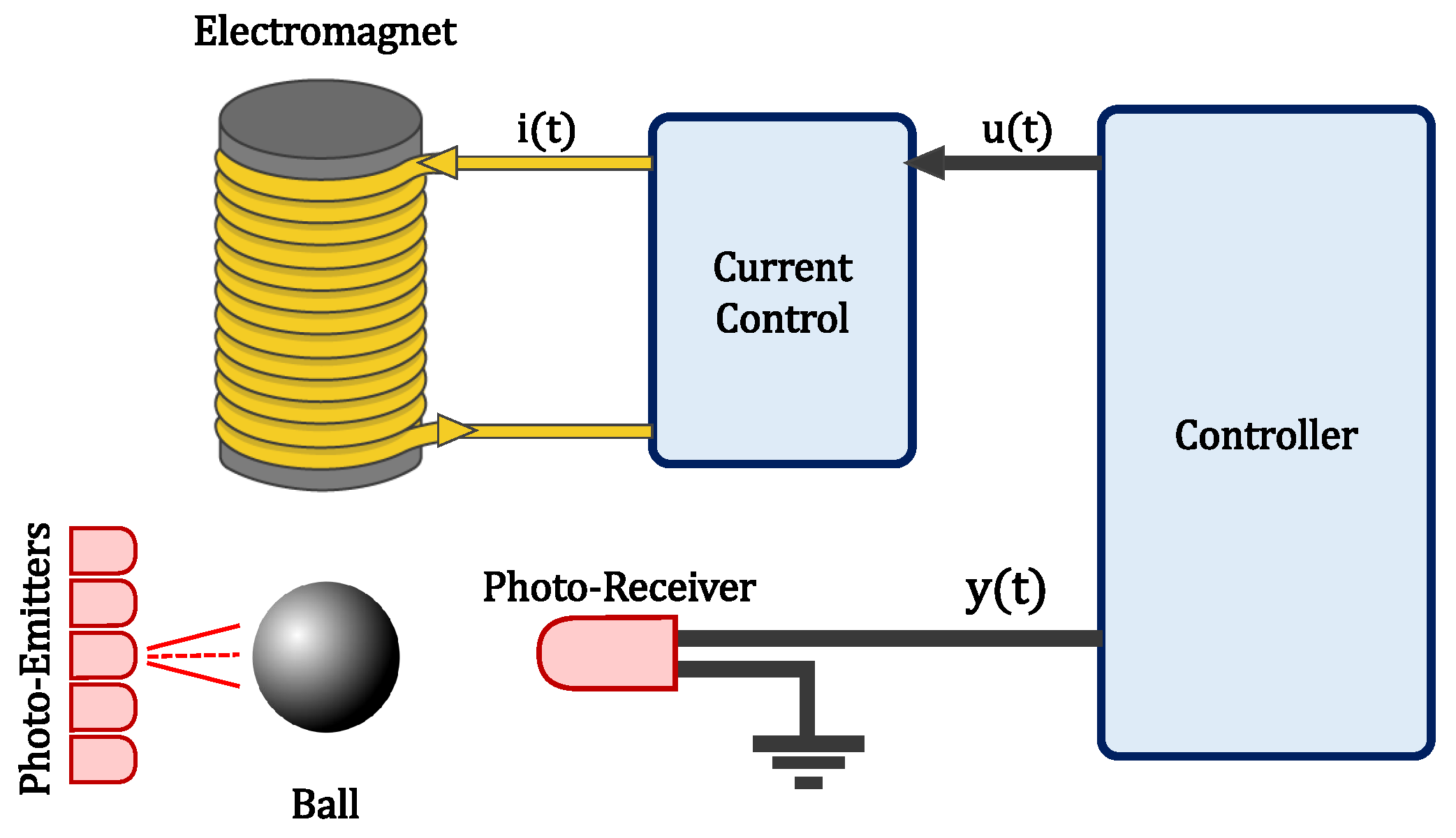
2. The Magnetic Levitation System and Problem Formulation

2.1. The Nonlinear Model

Let us consider the well known dynamic model of the magnetic levitation system shown in Figure 1:

$$\begin{array}{ccc}\hfill m\ddot{y}\left(t\right)& =& mg-\frac{K{i}^2\left(t\right)}{y^2\left(t\right)}\hfill \end{array}$$

(1)

$$\begin{array}{ccc}\hfill i\left(t\right)& =& Cu\left(t\right)\hfill \end{array}$$

(2)

in which m denotes the mass of the magnetic sphere, g defines the gravitational acceleration, $y\left(t\right)$ represents the measurable distance between the metallic sphere and the electromagnet, $u\left(t\right)$ represents the control input voltage, C is the coefficient expressing the ratio between the input voltage and the current across the coil $i\left(t\right)$ and K denotes a fixed-value parameter relating the mutual inductance of the sphere and coupling coefficients. Upon substituting (2) in (1) and carrying out a normalisation procedure, we obtain:

$$\ddot{y}\left(t\right)=g-\frac{K{C}^2}{m}\frac{u^2\left(t\right)}{y^2\left(t\right)}$$

(3)

By defining parameter $\beta =\frac{K{C}^2}{m}$ and substituting this expression in (3), we obtain:

$$\ddot{y}\left(t\right)=g-\beta \frac{u^2\left(t\right)}{y^2\left(t\right)}$$

(4)

2.2. Tangent Linearisation

Let us also consider the tangent linearisation of Equation (4) by means of a first order approximation of the Taylor series expansion around the following arbitrary unstable equilibrium point:

$$y=Y,\dot{Y}=0,\ddot{Y}=0,u=U\left(Y\right)=\sqrt{\frac{g}{\beta }}Y$$

(5)

The dynamic behaviour of the magnetic levitation system (4) can be described by the following nonlinear differential equation:

$$F(\ddot{y}\left(t\right),y\left(t\right),u\left(t\right))=\ddot{y}\left(t\right)-g+\beta \frac{u^2\left(t\right)}{y^2\left(t\right)}=0$$

(6)

It is assumed, first, that the dynamic system (6) is acting at its equilibrium point (5). This translates to the following:

$$F(\ddot{Y}=0,y=Y,u=U)=-g+\beta \frac{U^2}{Y^2}=0$$

(7)

If the system (6) is now subjected to a perturbation, it will go on to act in the point $y\left(t\right)=Y+y_{\delta }\left(t\right)$ and $u\left(t\right)=U+u_{\delta }\left(t\right)$, where $y_{\delta }\left(t\right)$ and $u_{\delta }\left(t\right)$ represent the effects caused by the cited perturbation. In this case, Equation (6) can be expanded by means of the Taylor series expansion around the equilibrium point (5), resulting in the following:

$$\begin{array}{ccc}\hfill & & F(\ddot{Y}\left(t\right)+{\ddot{y}}_{dd\delta }\left(t\right),Y+y_{\delta }\left(t\right),U+u_{\delta }\left(t\right))=\underset{=0\mathrm{from}\left(7\right)}{\underbrace{F(\ddot{Y}=0,Y,U)}}+{\left.\frac{\partial F\left(t\right)}{\partial \ddot{y}\left(t\right)}\right|}_{(0,Y,U)}{\ddot{y}}_{\delta }\left(t\right)+\hfill \\ & & +{\left.\frac{\partial F\left(t\right)}{\partial y\left(t\right)}\right|}_{(0,Y,U)}{y}_{\delta }\left(t\right)+{\left.\frac{\partial F\left(t\right)}{\partial u\left(t\right)}\right|}_{(0,Y,U)}{u}_{\delta }\left(t\right)+H.O.T.=0\hfill \end{array}$$

(8)

If the aforementioned perturbations are small enough, the Taylor expansion (8) can be limited disregarding those terms in which their powers or products appear (i.e., the H.O.T.), taking also the partial derivatives at the nominal operating point. Then, it results in the following:

$$\begin{array}{ccc}\hfill & & F(\ddot{Y}\left(t\right)+{\ddot{y}}_{dd\delta }\left(t\right),Y+y_{\delta }\left(t\right),U+u_{\delta }\left(t\right))\simeq {\left.\frac{\partial F\left(t\right)}{\partial \ddot{y}\left(t\right)}\right|}_{(0,Y,U)}{\ddot{y}}_{\delta }\left(t\right)+{\left.\frac{\partial F\left(t\right)}{\partial y\left(t\right)}\right|}_{(0,Y,U)}{y}_{\delta }\left(t\right)+\hfill \\ & & +{\left.\frac{\partial F\left(t\right)}{\partial u\left(t\right)}\right|}_{(0,Y,U)}{u}_{\delta }\left(t\right)=0\hfill \end{array}$$

(9)

which represents a linear equation of constant coefficients. Operating with Equations (5) and (9), and rearranging terms, one obtains the resulting first order approximation of the Taylor series expansion of the system (4) around the equilibrium point (5):

$${\ddot{y}}_{\delta }\left(t\right)=-C_U{u}_{\delta }\left(t\right)+C_Y{y}_{\delta }\left(t\right)$$

(10)

where $C_U={\left.\frac{\partial F\left(t\right)}{\partial u\left(t\right)}\right|}_{(0,Y,U)}=2\beta \frac{U}{Y^2}$, $C_Y=-{\left.\frac{\partial F\left(t\right)}{\partial y\left(t\right)}\right|}_{(0,Y,U)}=2\beta \frac{U^2}{Y^3}$, and the incremental variables of the linearised system are represented by $y_{\delta }\left(t\right)=y\left(t\right)-Y$, ${\dot{y}}_{\delta }\left(t\right)=\dot{y}\left(t\right)-\dot{Y}=\dot{y}\left(t\right)$, ${\ddot{y}}_{\delta }\left(t\right)=\ddot{y}\left(t\right)-\ddot{Y}=\ddot{y}\left(t\right)$ and $u_{\delta }\left(t\right)=u\left(t\right)-U$.

2.3. Flatness of the Linearised Magnetic Levitation System

In general, a SISO system is said to be flat if there exists a special endogenous output, called the flat output, which is a function of the system states and, possibly, of a finite number of their time derivatives, such that, in turn, all system variables (states, inputs, outputs) can be expressed solely in terms of the flat output and a finite number of its time derivatives [21]. The relation between flatness and controlability is quite simple in the context of linear time invariant SISO systems [22]: controlability and flatness are equivalent. Flatness property is particularly advantageous for solving trajectory planning problems and asymptotic set-point following control [23]. Upon studying the aforementioned linear dynamical model of the MLS obtained in Equation (10), it will be observed that the linearised system is flat with a flat output defined by the incremental distance between the ball and the electromagnet, denoted by $y_{\delta }\left(t\right)$. Indeed, all the system variables in the linearised model, i.e., the incremental states and the incremental control input, can be expressed as differential functions of the incremental flat output. In other words, they are expressible as functions of the incremental flat output $y_{\delta }\left(t\right)$ and a finite number of its time derivatives:

$$u_{\delta }\left(t\right)=-\frac{1}{C_U}{\ddot{y}}_{\delta }\left(t\right)+\frac{C_Y}{C_U}{y}_{\delta }\left(t\right)$$

(11)

2.4. Problem Formulation

Consider the magnetic levitation system, which is modelled by employing Equation (4) and approximately linearised by means of the linear dynamic model described in Equation (10). We, then, develop a robust control law such that it forces the metallic sphere to track a desired rest-to-rest smooth reference trajectory for the distance between the metallic sphere and the electromagnet, $y^{*}\left(t\right)=Y+y_{\delta }^{*}\left(t\right)$, from an initial equilibrium value, $y^{*}\left(0\right)=Y+y_{\delta }^{*}\left(0\right)$ towards a final desired position $y\left(t_f\right)=Y+y_{\delta }^{final}\left(t_f\right)$ within a given prescribed time interval $[0,t_f]$. The designed controller will act robustly in spite of large initial errors, the ignored non-linearities in the linearisation process, the presence of parametric uncertainties and the measurement noises.

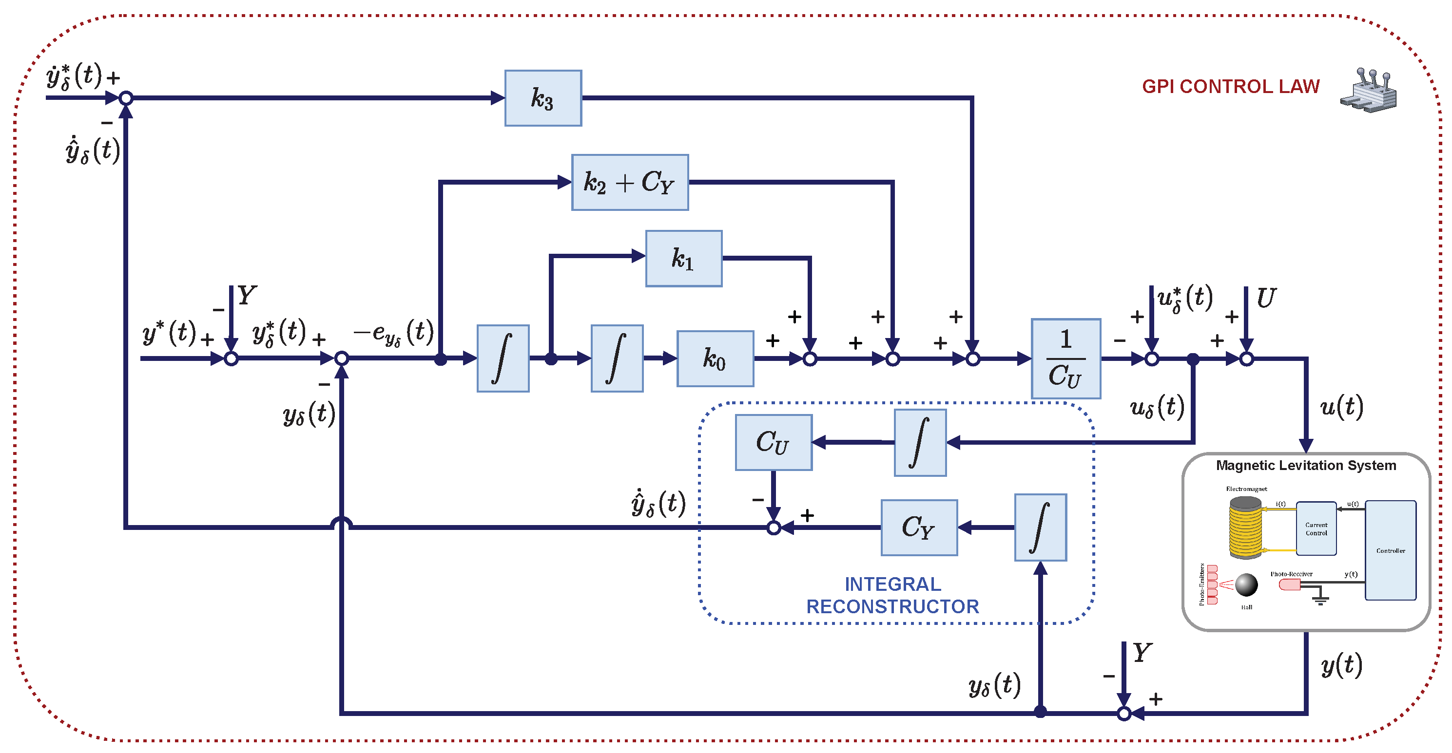
3. Generalised Proportional Integral Controller Design

Linear output feedback controllers for linear systems provided by GPI controllers are more than satisfactory. These controllers are also useful, effective and suitable for systems with nonlinear dynamics, such as the specific case of MLS. Their basis is the defective integral reconstruction of the state, which, a priori, ignores the effects of unknown initial conditions and the effect of possible classical perturbation inputs (constant and low order time polynomial errors, i.e., ramps and parabolic signals). Another of their starting points is the key observation that it is possible to integrally parameterise states of observable linear systems as a function that depends only on their inputs and outputs (encompasses the linear combination of inputs, outputs and a finite number of iterated integrals of signals). Subsequently, integral reconstruction errors are counteracted by employing an appropriate linear controller that contains enough iterated integrals of the tracking error or the input error.

3.1. A Flatness-Based Pole Placement Approach for Stabilisation

We shall now consider the linearised dynamics of the magnetic levitation system provided by Equation (10), in which the objective is to track a rest-to-rest position incremental reference trajectory for the distance between the ball and the electromagnet, denoted as $y_{\delta }^{*}\left(t\right)$. If there is an open loop incremental control input voltage, $u_{\delta }^{*}\left(t\right)$, that ideally obtains the tracking of the desired smooth reference trajectory for the distance between the ball and the electromagnet $y_{\delta }^{*}\left(t\right)$ by means of appropriate initial conditions, then it clearly satisfies the following expression:

$${\ddot{y}}_{\delta }^{*}\left(t\right)=-C_U{u}_{\delta }^{*}\left(t\right)+C_Y{y}_{\delta }^{*}\left(t\right)$$

(12)

The subtraction of expressions (10) and (12) yields the following second order dynamics for the incremental tracking output error $e_{y_{\delta }}\left(t\right)=y_{\delta }\left(t\right)-y_{\delta }^{*}\left(t\right)$:

$${\ddot{e}}_{y_{\delta }}\left(t\right)-C_Y{e}_{y_{\delta }}\left(t\right)=-C_U(u_{\delta }\left(t\right)-u_{\delta }^{*}\left(t\right))$$

(13)

A direct exact linearisation-based feedback controller that regulates the incremental output error $e_{y_{\delta }}\left(t\right)$ to zero is provided by the following expression (for additional details of the flatness approach, see [24,25]):

$$\begin{array}{cc}\hfill & u_{\delta }\left(t\right)=u_{\delta }^{*}\left(t\right)-\frac{1}{C_U}[-k_3({\dot{y}}_{\delta }\left(t\right)-{\dot{y}}_{\delta }^{*}\left(t\right))-(k_2+C_Y)(y_{\delta }\left(t\right)-y_{\delta }^{*}\left(t\right))\hfill \\ \hfill & -k_1{\int }_0^t(y_{\delta }\left(\sigma \right)-y_{\delta }^{*}\left(\sigma \right))d\sigma ]\hfill \end{array}$$

(14)

where $u_{\delta }^{*}\left(t\right)$ is the desired incremental control input voltage, and if the set of coefficients $\{k_3,k_2,k_1\}$ is appropriately selected, then the preceding flatness-based controller imposes stable closed-loop dynamics on the incremental tracking output error $e_{y_{\delta }}\left(t\right)$:

$$e_{y_{\delta }}^{\left(3\right)}\left(t\right)+k_3{\ddot{e}}_{y_{\delta }}\left(t\right)+k_2{\dot{e}}_{y_{\delta }}\left(t\right)+k_1{e}_{y_{\delta }}\left(t\right)=0$$

(15)

If the set of coefficients $\{k_3,k_2,k_1\}$ is designed in such a way that the closed loop characteristic polynomial

$$s^{\left(3\right)}+k_3{s}^2+k_{2}s+k_1=0$$

(16)

is composed of a third degree Hurwitz polynomial whose roots are located sufficiently far into the left half on the complex plane, then the trajectories of the incremental output error $e_{y_{\delta }}\left(t\right)$, and their corresponding time derivatives exponentially converge to zero. Upon studying the control law proposed in (14) it will be noted that knowledge of the incremental velocity of the magnetic ball, ${\dot{y}}_{\delta }\left(t\right)$, is required, signifying that a variable of this nature must either be measured or estimated by an observer. In practise, the estimation is attained by means of online calculations based on high frequency samples of the trajectory of the incremental position variable. The signal is usually quite noisy, and low pass filters are, therefore, required in order to smooth them, thus leading to the well-known dynamic delays that affect the tracking of the position of the ball as regards its performance and accuracy. The aforementioned problems can, however, be avoided through the use of a GPI controller.

3.2. Using GPI to Locally Control the Magnetic Levitation System

In this section, we once again solve the aforementioned control problem by assuming that only the position between the magnetic ball and the electromagnet is available for measurements and that some dynamics of the original system are unknown. As explained in Section 3.1, during the development of the GPI controller, the computation of the estimate incremental velocity of the magnetic ball, ${\dot{\widehat{y}}}_{\delta }\left(t\right)$, needs only a linear combination of iterated integrals of the incremental control input voltage, $u_{\delta }\left(t\right)$, and the incremental distance between the ball and the electromagnet, $y_{\delta }\left(t\right)$, thus avoiding the aforementioned problems. Indeed, we suppose that the incremental position of the ball $y_{\delta }\left(t\right)$ and the incremental input voltage, $u_{\delta }\left(t\right)$, are the only variables available for measurement. In this case, the estimation of the incremental velocity of the magnetic ball, ${\dot{\widehat{y}}}_{\delta }\left(t\right)$ is directly determined by the integration of Equation (10), as follows:

$${\dot{y}}_{\delta }\left(t\right)=-C_U{\int }_0^t{u}_{\delta }\left(\sigma \right)d\sigma +C_Y{\int }_0^t{y}_{\delta }\left(\sigma \right)d\sigma +{\dot{y}}_{\delta }\left(0\right)$$

(17)

where ${\dot{y}}_{\delta }\left(0\right)$ denotes the value of the incremental velocity of the magnetic ball at time $t=0$. However, this information is not usually known, and we can suppose only that this value is known in the case in which the magnetic ball starts moving with a null incremental velocity. We, therefore, assume that we have no knowledge of the variable ${\dot{y}}_{\delta }\left(0\right)$. Bearing in mind the simplicity of Equation (17), we opt to use the following structural estimation for the incremental velocity of the magnetic ball, ${\dot{\widehat{y}}}_{\delta }\left(t\right)$:

$${\dot{\widehat{y}}}_{\delta }\left(t\right)=-C_U{\int }_0^t{u}_{\delta }\left(\sigma \right)d\sigma +C_Y{\int }_0^t{y}_{\delta }\left(\sigma \right)d\sigma$$

(18)

which has the advantage that it can be obtained by using only a linear combination of the integral of the incremental position of the ball, $y_{\delta }\left(t\right)$, and the integral of the incremental input voltage, $u_{\delta }\left(t\right)$, thus avoiding the use of low pass filters to smooth the noise component of the incremental position of the ball and the subsequent online calculations based on high frequency samples of the filtered incremental position of the ball, which usually entail dynamic delays that influence the accuracy and the performance of the stabilisation and tracking tasks. The exact relationship between the actual value of the incremental velocity of the magnetic ball and its corresponding structural estimation is obtained from expressions (17) and (18) as follows:

$${\dot{y}}_{\delta }\left(t\right)={\dot{\widehat{y}}}_{\delta }\left(t\right)+{\dot{y}}_{\delta }\left(0\right)$$

(19)

Bearing in mind the results obtained in expressions (18) and (19), and the problems described in the aforementioned control law (14) owing to the fact that only the position between the magnetic ball and the electromagnet is available for measurement, we present the following modified feedback control law. This control law is depicted in Figure 2 and includes an integral error term and a double integral error term in order to make it robust to constant and possible unmodelled ramp perturbation loads:

$$\begin{array}{cc}\hfill & u_{\delta }\left(t\right)=u_{\delta }^{*}\left(t\right)-\frac{1}{C_U}[-k_3({\dot{\widehat{y}}}_{\delta }\left(t\right)-{\dot{y}}_{\delta }^{*}\left(t\right))-(k_2+C_Y)(y_{\delta }\left(t\right)-y_{\delta }^{*}\left(t\right))\hfill \\ \hfill & -k_1{\int }_0^t(y_{\delta }\left(\sigma \right)-y_{\delta }^{*}\left(\sigma \right))d\sigma -k_0{\int }_0^t{\int }_0^{\lambda }(y_{\delta }\left(\sigma \right)-y_{\delta }^{*}\left(\sigma \right))d\sigma d\lambda ]\hfill \\ \hfill & u_{\delta }^{*}\left(t\right)=-\frac{1}{C_U}\left({\ddot{y}}_{\delta }^{*}\left(t\right)-C_Y{y}_{\delta }^{*}\left(t\right)\right)\hfill \\ \hfill & {\dot{\widehat{y}}}_{\delta }\left(t\right)=-C_U{\int }_0^t{u}_{\delta }\left(\sigma \right)d\sigma +C_Y{\int }_0^t{y}_{\delta }\left(\sigma \right)d\sigma \hfill \end{array}$$

(20)

When the modified controller provided by Equation (20) is implemented in the magnetic levitation system defined in Equation (4), we obtain the following linear perturbed dynamics:

$${\ddot{e}}_{y_{\delta }}\left(t\right)+k_3{\dot{e}}_{y_{\delta }}\left(t\right)+k_2{e}_{y_{\delta }}\left(t\right)+k_1{\int }_0^t{e}_{\delta }\left(\sigma \right)d\sigma +k_0{\int }_0^t{\int }_0^{\lambda }{e}_{\delta }\left(\sigma \right)d\sigma d\lambda =k_3{\dot{y}}_{\delta }\left(0\right)$$

(21)

and after differentiating (21) twice, the following fourth-order linear incremental tracking output error dynamics is obtained:

$$e_{y_{\delta }}^{\left(4\right)}\left(t\right)+k_3{e}_{y_{\delta }}^{\left(3\right)}\left(t\right)+k_2{\ddot{e}}_{y_{\delta }}\left(t\right)+k_1{\dot{e}}_{\delta }\left(t\right)+k_0{e}_{\delta }\left(t\right)=0$$

(22)

which clearly has the origin ($e_{y_{\delta }}\left(t\right)=y_{\delta }\left(t\right)-y_{\delta }^{*}\left(t\right)=0$) as an asymptotically exponential equilibrium point, independently of the values of the initial conditions of the system. The set of design parameters $\{k_3,k_2,k_1,k_0\}$ is selected so as to render the closed-loop characteristic polynomial,

$$p\left(s\right)=s^{\left(4\right)}+k_3{s}^{\left(3\right)}+k_2{s}^2+k_{1}s+k_0=0$$

(23)

in a fourth-degree Hurwitz polynomial with desirable roots. In order to specify the parameters, we can choose to locate the desired loop poles in the left half of the complex plane. The controller parameters were chosen so as to obtain the following desired closed-loop characteristic polynomial:

$$p_{des}\left(s\right)={\left(s^2+2{\xi }_d{\omega }_{nd}+{\omega }_{nd}^2\right)}^2=0$$

(24)

where ${\xi }_d$ and ${\omega }_{nd}$ are positive quantities. The coefficients $\{k_3,k_2,k_1,k_0\}$ are, therefore, obtained by equating each term of Equation (23) with those of Equation (24), which are given by:

$$k_3=4{\xi }_d{\omega }_{nd};k_2=4{\xi }_d^2{\omega }_{nd}^2+2{\omega }_{nd}^2;k_1=4{\xi }_d{\omega }_{nd}^3;k_0={\omega }_{nd}^4$$

(25)

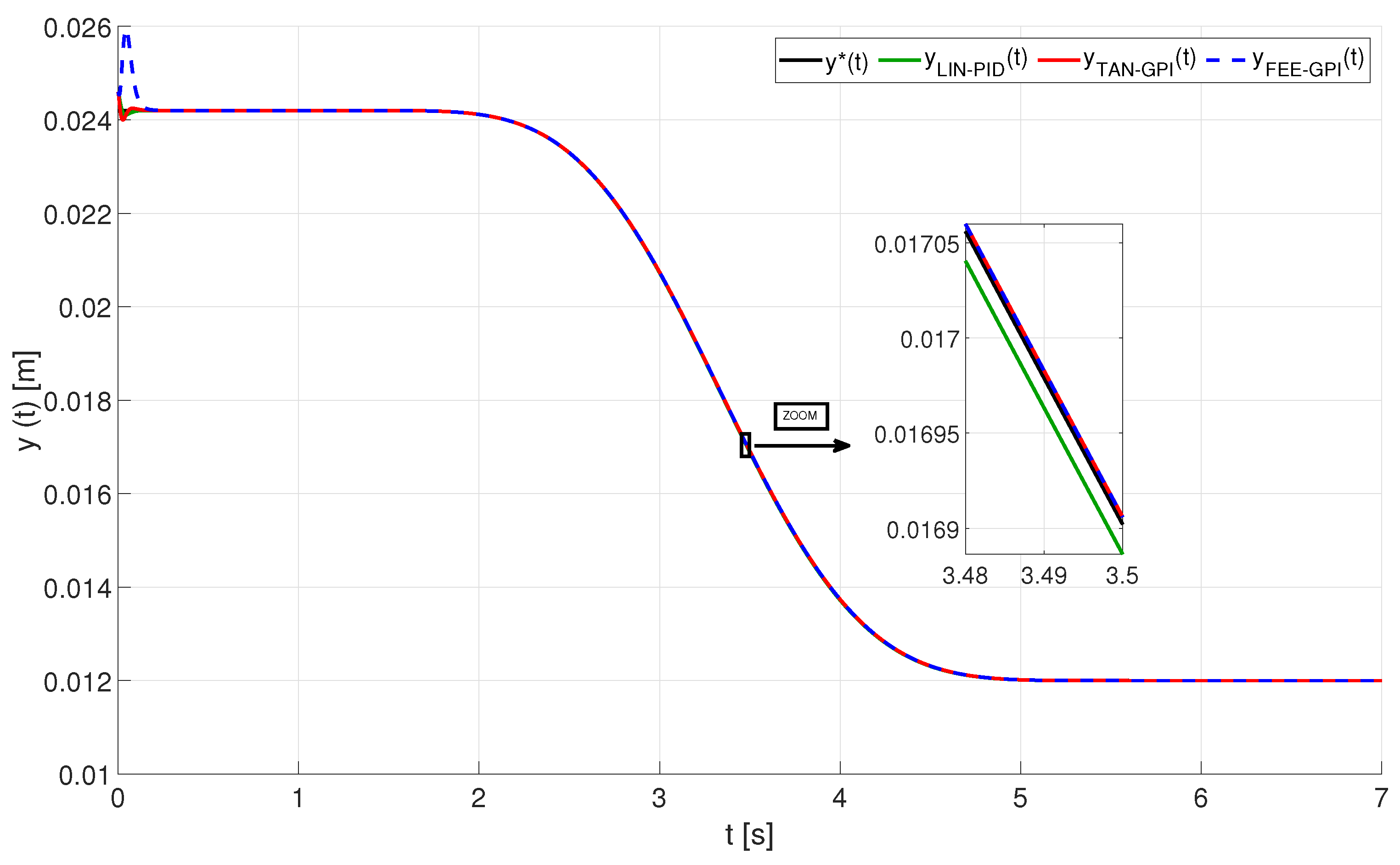
4. Computer Simulations

Numerical simulations made it possible to verify that the proposed controller achieved accurate stabilisation and tracking results. As explained in previous sections, the principal problems associated with the control of a MLS are its strong unstable behaviour in open-loop and the presence of significant non-linearities and uncertainties. In the proposed computer simulations, several cases were developed in order to make a comparison between the GPI control based on tangent linearisation presented in this paper (denoted in the graphs as TAN-GPI and represented in red colour), a standard linear PID control [26] (LIN-PID, green colour), and the exact feedforward-GPI controller [19] (FEE-GPI, blue colour). The comparison was carried out on the basis of the rapid stabilisation and convergence of the tracking errors, smooth transient responses, low control effort and robustness to the following cases: (i) initial position errors; (ii) ignored non-linearities in the linearisation process; (iii) the presence of parametric uncertainties; and (iv) measurement noises. We considered the following values for the MLS platform in the numerical simulations:

$$\begin{array}{ccc}& & g=9.81\left[\frac{m}{s^2}\right];C=1.05\left[\frac{A}{V}\right];m=0.02\left[kg\right];K=2.48315625·{10}^{-5}\left[\frac{N{m}^2}{A^2}\right]\hfill \\ & & \beta =\frac{K{C}^2}{m}=0.00136884\left[\frac{N{m}^2}{kg{V}^2}\right]\hfill \end{array}$$

(26)

The sampling time was set at $0.001s$. The desired fourth-degree Hurwitz polynomial (23) was set in order to exhibit the following parameters: ${\xi }_d=1$ and ${\omega }_{nd}=70$. These values were chosen to satisfy the Haykin’s condition [27], and based on them, the set of parameters $\{k_3,k_2,k_1,k_0\}$ was calculated according to (25). The positions of the poles in the other two controllers implemented for the comparison, the linear PID and the feedforward-GPI, were also set at $-70$. The equilibrium point used to determine parameters $C_U$ and $C_Y$ of the tangent linearisation of the system was set at $Y=0.0246\left[m\right]$ and $U=2.0825\left[V\right]$. The magnetic ball started the simulations in a initial position equal to $y\left(0\right)=0.0246\left[m\right]$, and in all of the following simulations, the magnetic ball was commanded to follow a desired smooth Bezier’s trajectory, defined by $y^{*}\left(t\right)$, which transfers the magnetic ball from an initial equilibrium value of $y^{*}\left(t_i\right)={\overline{y}}_i=0.0242\left[m\right]$ to a final equilibrium value of $y^{*}\left(t_f\right)={\overline{y}}_f=0.0120\left[m\right]$ during a finite interval of the form $\left[t_i,t_f\right]=[1.00,6.00]s$. This reference trajectory is defined as:

$$y^{*}\left(t\right)={\overline{y}}_i+\left({\overline{y}}_f-{\overline{y}}_i\right)·\varphi (t,t_f,t_i)$$

(27)

where $t_i$, $t_f$, ${\overline{y}}_i$ and ${\overline{y}}_f$ are defined by the user and $\varphi (t,t_i,t_f)$ is defined as an interpolation function between the values 0 and 1 during the interval $\left[t_i,t_f\right]$. For example, we selected the following 16th-order Bezier polynomial:

$$\varphi (t,t_i,t_f)=\left\{\begin{array}{c}0\mathrm{for}t<t_i\hfill \\ {\left[\frac{t-t_i}{t_f-t_i}\right]}^8·\left[r_1-r_2\left(\frac{t-t_i}{t_f-t_i}\right)+r_3{\left(\frac{t-t_i}{t_f-t_i}\right)}^2-\dots +r_9{\left(\frac{t-t_i}{t_f-t_i}\right)}^8\right]\mathrm{for}{t}_i\le t\le t_f\hfill \\ 1\mathrm{for}t>t_f\hfill \end{array}\right.$$

(28)

where

$$\begin{array}{ccccc}{r}_1=12870& r_2=91520& r_3=288288& r_4=524160& r_5=600600\\ r_6=443520& r_7=205920& r_8=54912& r_9=6435& \end{array}$$

(29)

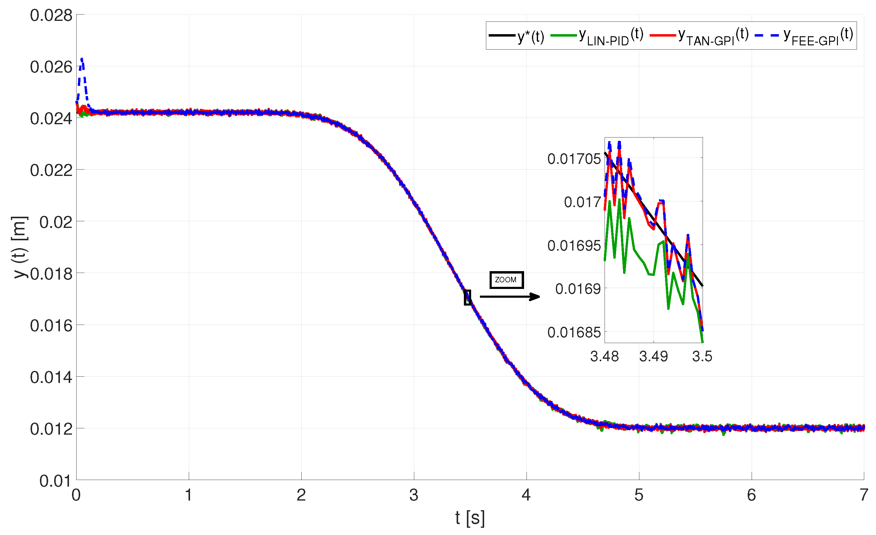
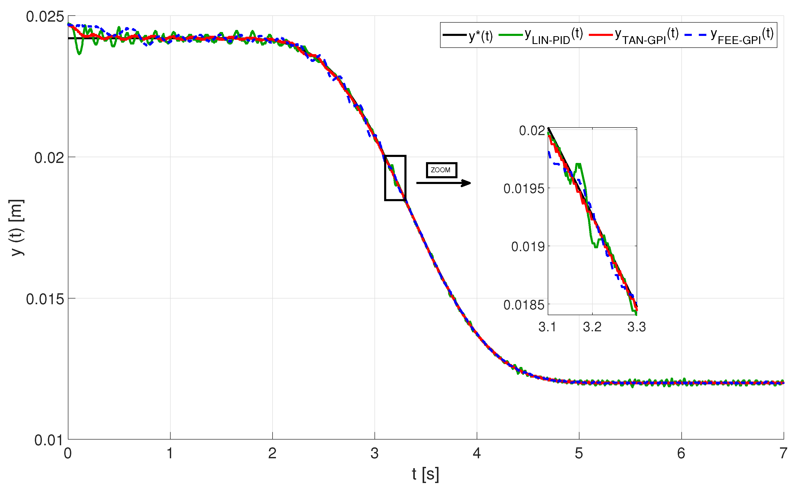
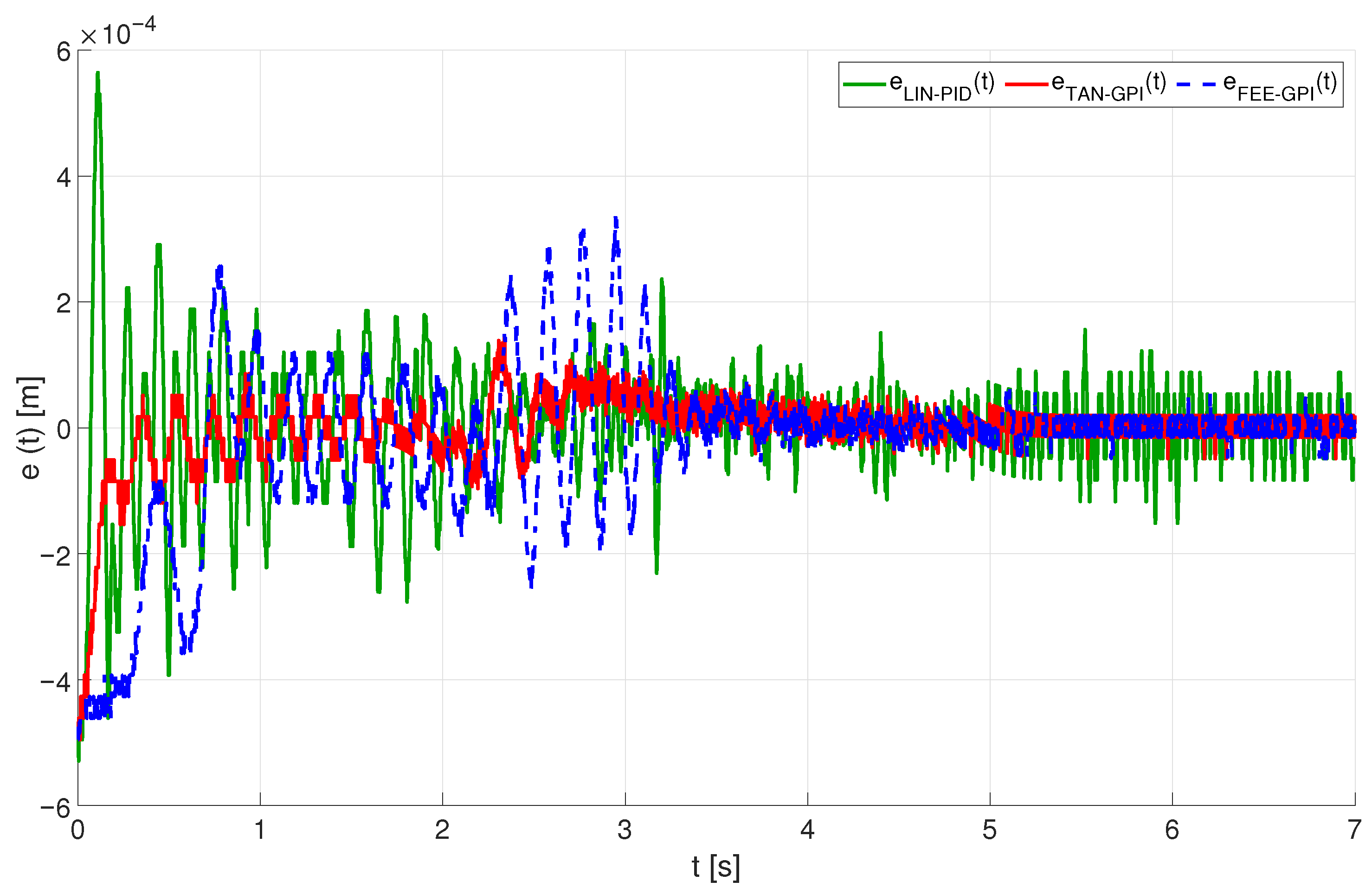
4.1. Tracking a Smooth Rest-to-Rest Trajectory

In this section, the computer simulation was carried out under almost ideal conditions (referred to as Test 1 or the nominal case), which implies that there were initial position errors and ignored non-linearities in the linearisation process. Figure 3 depicts the controlled evolution of the position of the magnetic ball using a linear PID, the feedforward-GPI and the GPI based on tangent linearisation when the motion of the magnetic ball started in a position that was significantly different from the desired trajectory. The different case studies proposed in this section illustrate that the main difficulties occurred at the beginning of the computer simulations. This is due to the circumstance of controlling a system with unstable open-loop dynamics, and that these kinds of systems tended to have a closed-loop response which was characterised by a significant overshoot around the initial time.

Figure 4 and Figure 5 illustrate the trajectory tracking error and the control input using the linear PID, the feedforward-GPI, and the proposed GPI for the nominal case (Test 1). As may be observed, although there were inaccuracies in the model owing to the initial position errors and the ignored non-linearities in the linearisation process, the three feedback controllers corrected the motion of the levitated ball and guided the position error to a small neighbourhood of zero. In the case of the PID, it will be noted that the behaviour of the tracking of the reference trajectory was worse (the error was significant in the central transition of the Bezier trajectory, from approximately second 3 to second 5). This will also be noted in the control effort, for which the proposed GPI controller responded better. In the case of the feedforward-GPI controller, a large initial error was observed in the trajectory tracking, which was reduced after the first instants thanks to the action of the GPI control law. The control effort was similar to the proposed controller, but the initial error weighted the performance down. Therefore, the GPI based on tangential linearisation obtained the best results.

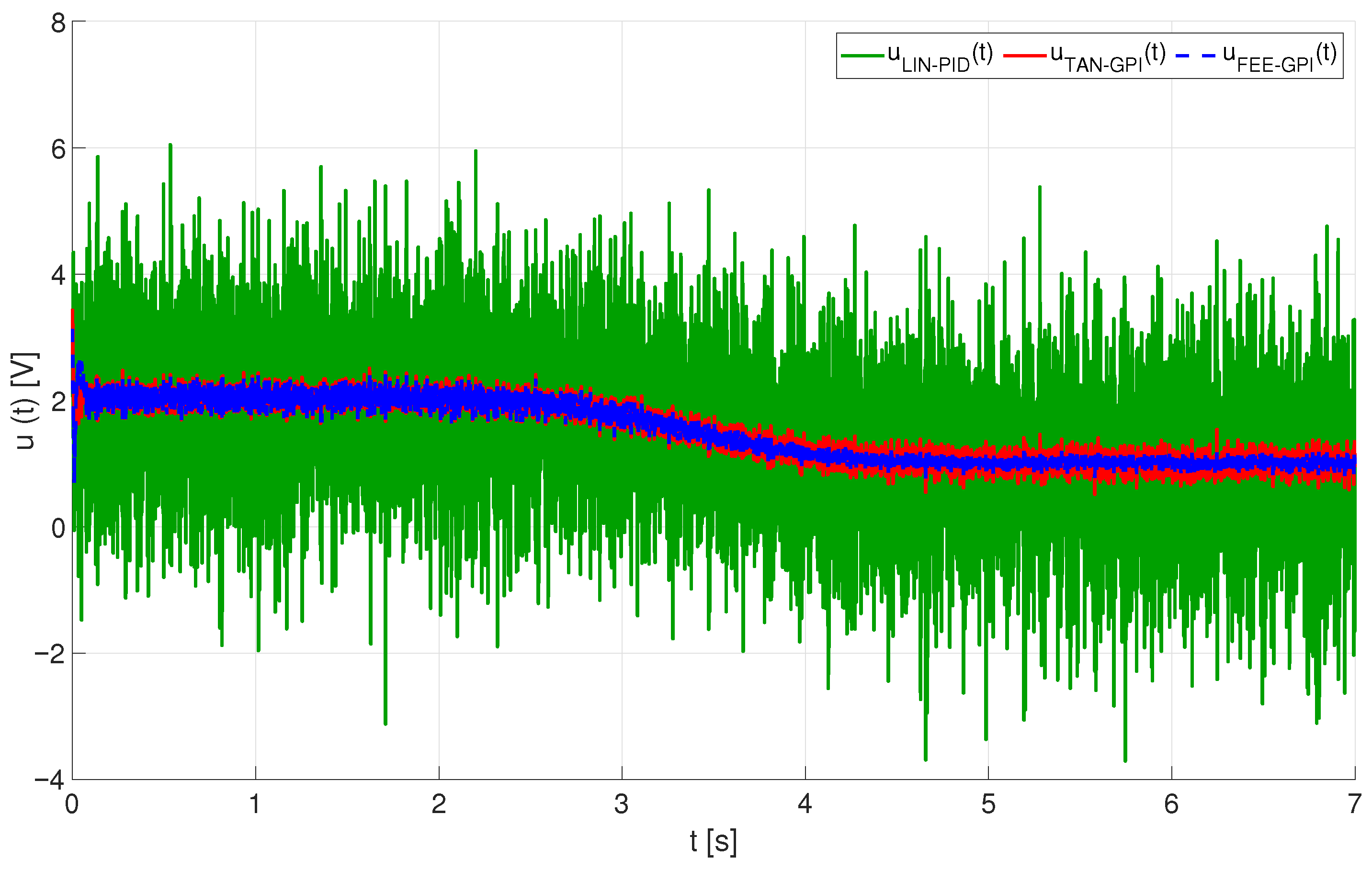
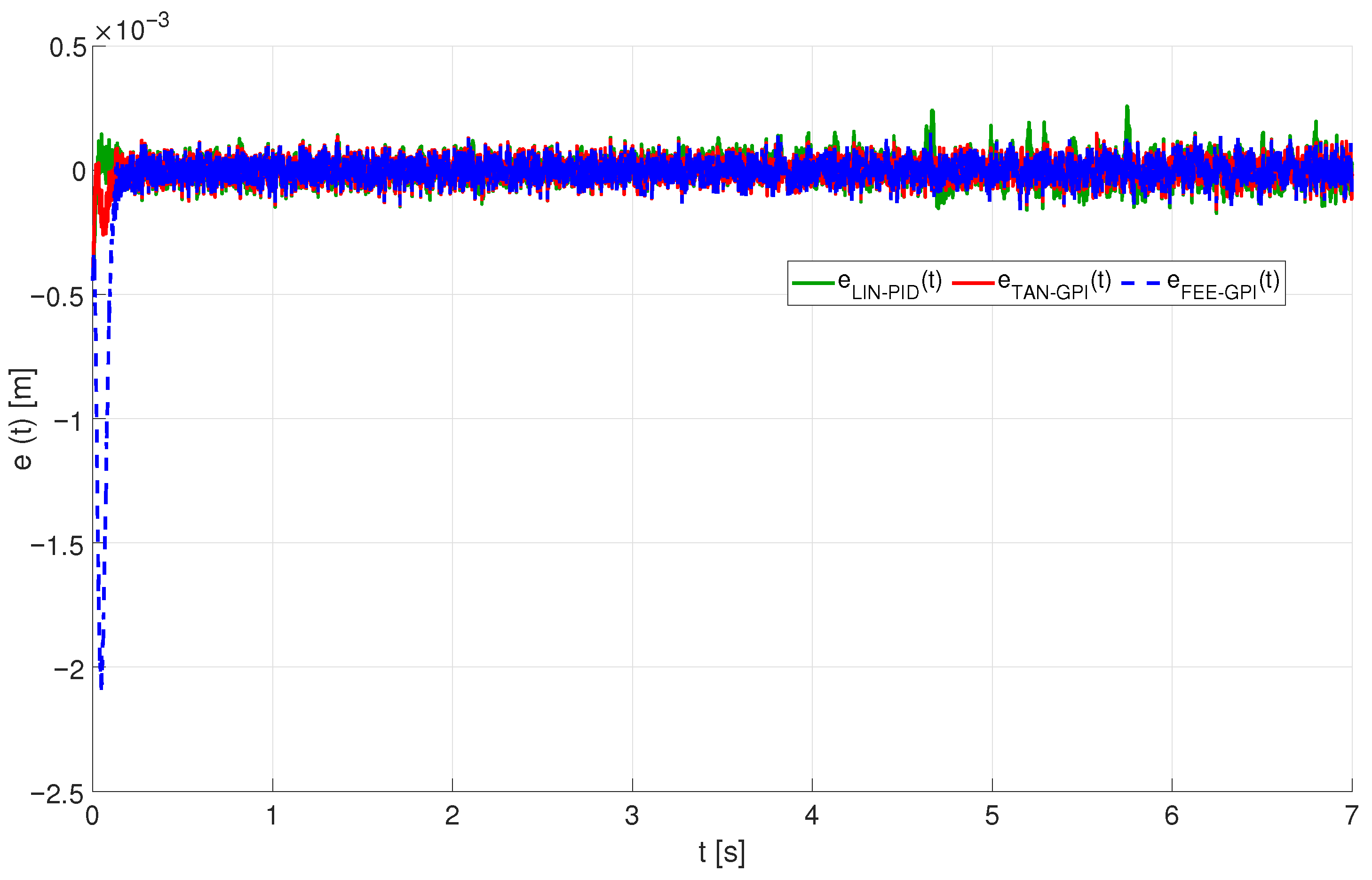
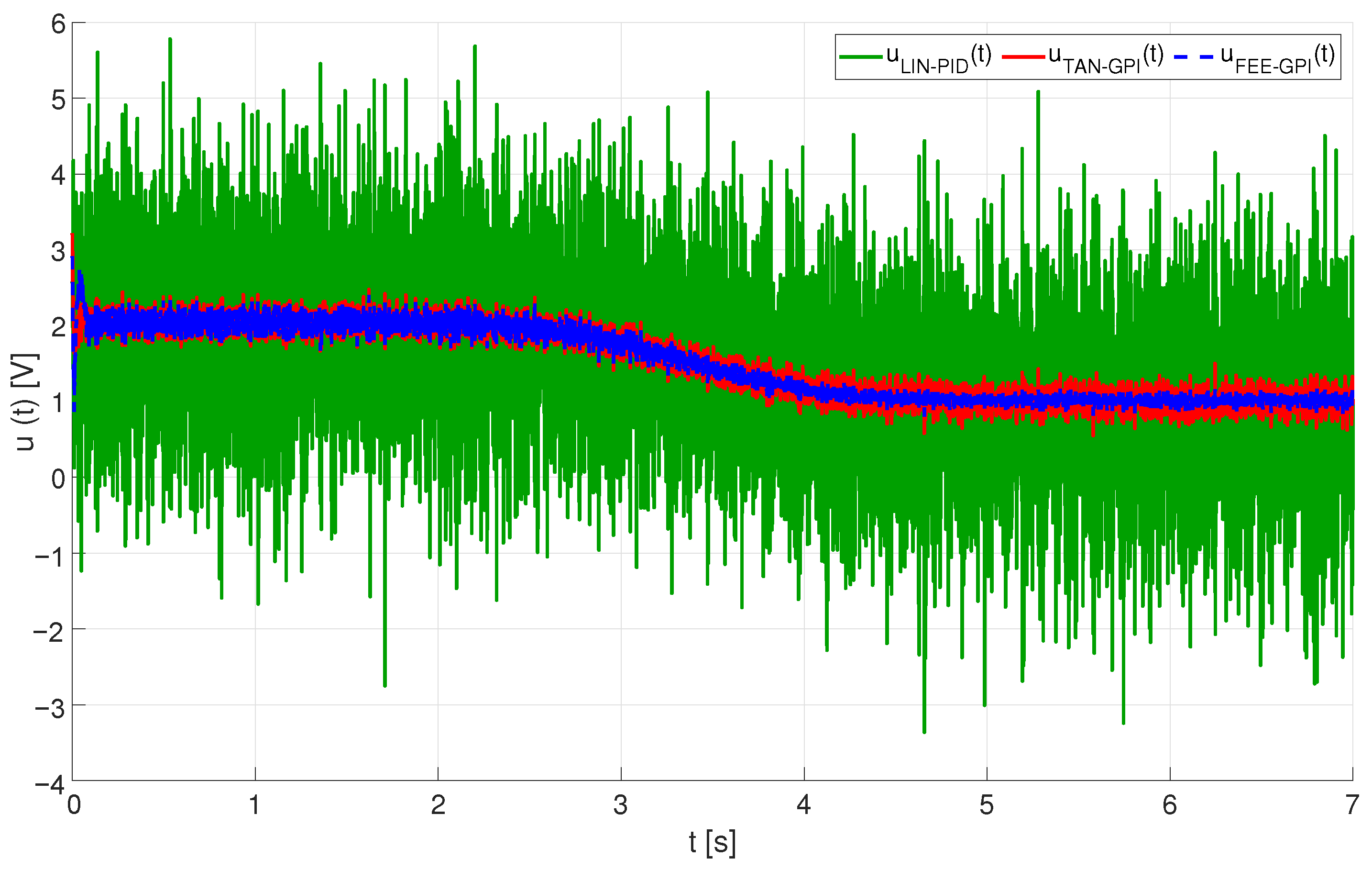
4.2. Robustness with Regard to Measurement Noises

We now present results concerning the robustness properties of the controllers with regard to measurement noises. In these simulations, we included an initial position error, the ignored non-linearities in the linearisation process, and the modification of two signals, the control input, $\widehat{u}\left(t\right)=u\left(t\right)+n_u\left(t\right)$ and the system’s output, $\widehat{y}\left(t\right)=y\left(t\right)+n_y\left(t\right)$), where $n_u\left(t\right)$ and $n_y\left(t\right)$, represent normally distributed random processes. Figure 6 illustrates the stabilisation and the trajectory tracking of the magnetic ball when the additive measurement noise standard deviations were $1·{10}^{-3}\left(n_u\left(t\right)\right)$ and $1.4·{10}^{-9}\left(n_y\left(t\right)\right)$, using the linear PID control, the feedforward-GPI and the proposed GPI control based-on tangent linearisation.

Despite the different disturbances included in the system, the proposed GPI control based on tangent linearisation, and with the same controller parameters used in the previous section, efficiently corrected the undesirable effects of the aforementioned perturbations. Moreover, it is again worth noting the better performance of the GPI controller with respect to the PID controller. This was even more evident if we analysed the error in both the trajectory tracking and the control input applied to the model, which are represented in Figure 7 and Figure 8, respectively.

It can be observed that the proposed GPI achieved a better approach to the vicinity of zero as regards the tracking error, thus achieving a more accurate trajectory tracking at the ball position when compared to the PID, and all this with a much lower control effort. The robustness to the presence of noise in the measurements was, therefore, better in the case of the GPI controller. If comparing the performance of the proposed GPI controller with the feedforward-GPI, we can again conclude that a faster reduction of the tracking error was reached with the new control scheme, thus obtaining a more accurate tracking of the reference trajectory. At the end of the simulation, the tracking error was limited to a proximity of zero of a similar order and with parallel control effort, so the feedforward-GPI also managed to be robust to noise, but overall, the proposed GPI was still superior to its feedforward counterpart.

4.3. Robustness with Regard to Controller Gain Mismatches

In this section, we simulated the behaviour of the closed loop system, assuming: that there were initial position errors, ignored non-linearities in the linearisation process, and the same measurement noise as that employed in Section 4.2. We now also assumed that the parameter $\beta$ was not precisely known and that the controllers were implemented with an estimated value ${\beta }_c$ (see Appendix A for details). We specifically conducted simulations in which an error of the order of 15% of the parameter ${\beta }_c$ was assumed (i.e., ${\beta }_c=1.15\beta$). Figure 9, Figure 10 and Figure 11 illustrate the results of the simulation carried out.

As may be observed, although there were disturbances of a different nature, the new feedback controller corrected the motion of the levitated ball and guided the position error to a small neighbourhood of zero, in addition to compensating for the error in the model parameter. The performance of the proposed controller was also better than the PID scheme in all respects. It is, however, worth mentioning that the PID also achieved stabilisation and trajectory tracking for the ball position, despite the simulated modelling error, although with lower accuracy and requiring a greater control effort. The initial error in feedforward-GPI trajectory tracking was even more pronounced in this last simulation test. Certainly, the tracking error ended up similarly bounded in a range close to zero, with the control effort decreasing as the simulation progressed. However, the overall performance of the feedforward-GPI was worse than the proposed new GPI. This way, the novel control scheme demonstrated a better performance in the three simulation tests.

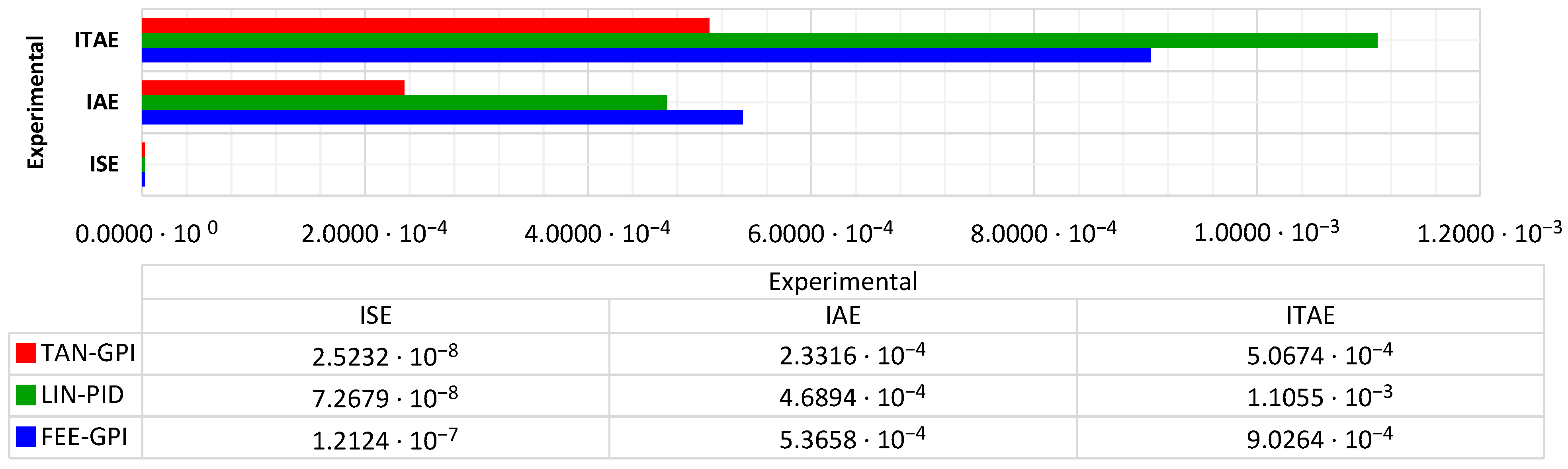
4.4. Comparison of the Controllers Based on Integral Criteria

We studied the performance of the control methods as regards integral criteria by employing the following performance indexes to express the performance of the control systems [28]: (i) ISE, $ISE={\int }_{t_A}^{t_B}{e}^2\left(t\right)\mathrm{d}t$; (ii) IAE, $IAE={\int }_{t_A}^{t_B}\left|e\left(t\right)\right|\mathrm{d}t$, and, (c) ITAE, $ITAE={\int }_{t_A}^{t_B}t·\left|e\left(t\right)\right|\mathrm{d}t$. The initial and final time of the simulation are denoted by values $t_A=0s$ and $t_B=7s$. All the tracking errors are uniformly dealt with by the ISE and the IAE criteria [29,30]. However, since time is a factor in the ITAE criterion, it heavily penalises errors that take place late in time, but ignores errors that take place early in time [31,32,33]. The results attained for ISE, IAE and ITAE are shown in Figure 12, which illustrates that the proposed GPI controller performs better than that to which it is compared (smaller values).

This concurs with the theoretical developments [34,35] in the three simulation tests, which were performed under almost ideal conditions (initial position error and ignored non-linearities in the linearisation process) and which are referred to as the nominal case (Test 1), the case including the conditions of Test 1 with measurement noise disturbances (Test 2), and the case including conditions of Test 2 with controller gain mismatches (Test 3). After comparing the simulation results achieved for the different control laws, the designed GPI control scheme results in an improvement of the behaviour of the MLS which is reflected in the aspects listed next: (1) an enhanced transient response; (2) an improved stabilisation with smaller trajectory tracking errors; (3) an increase of the robustness against noisy perturbation signals; (4) a better handling of modelling errors and environmental uncertainties; (5) a significant reduction of the steady-state error; and (6) less effort in the controller actions.

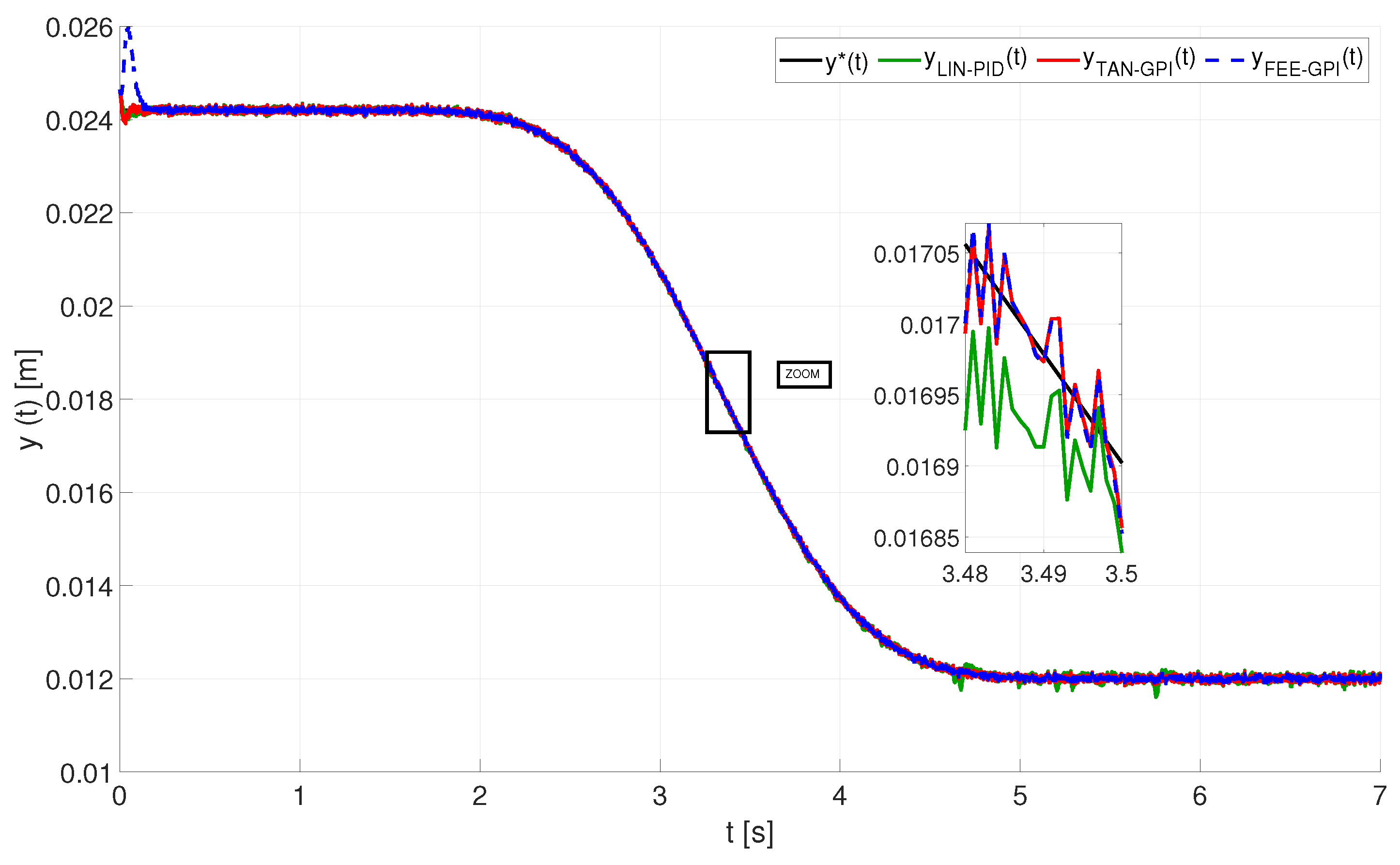
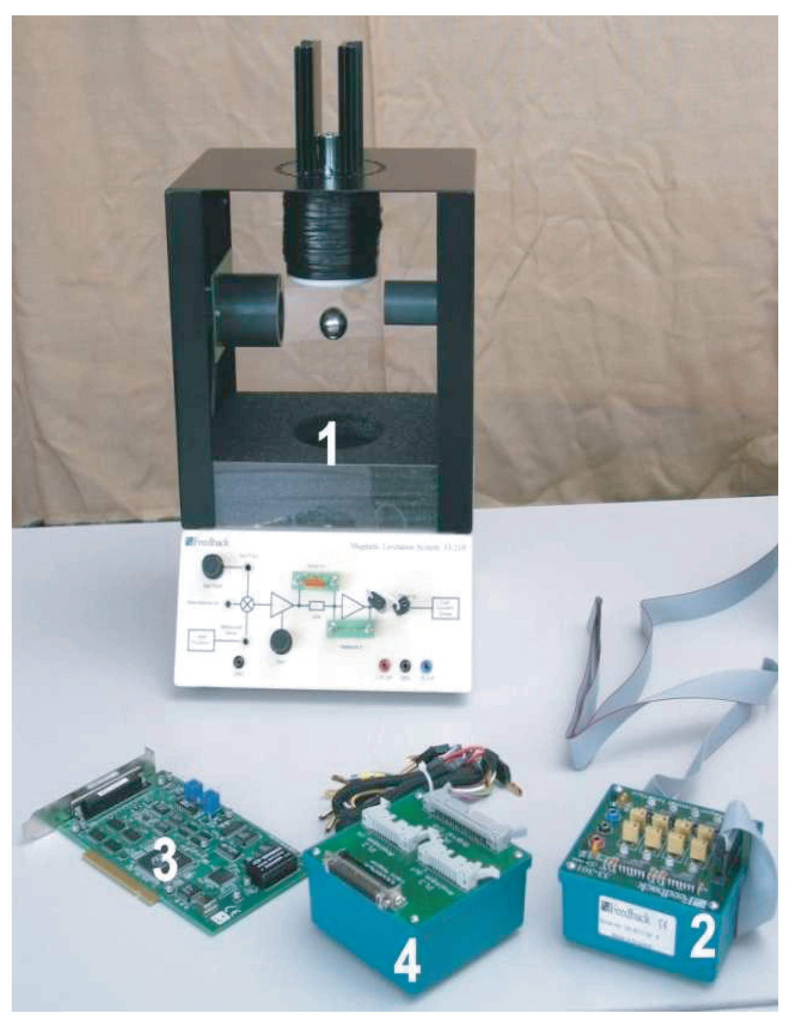
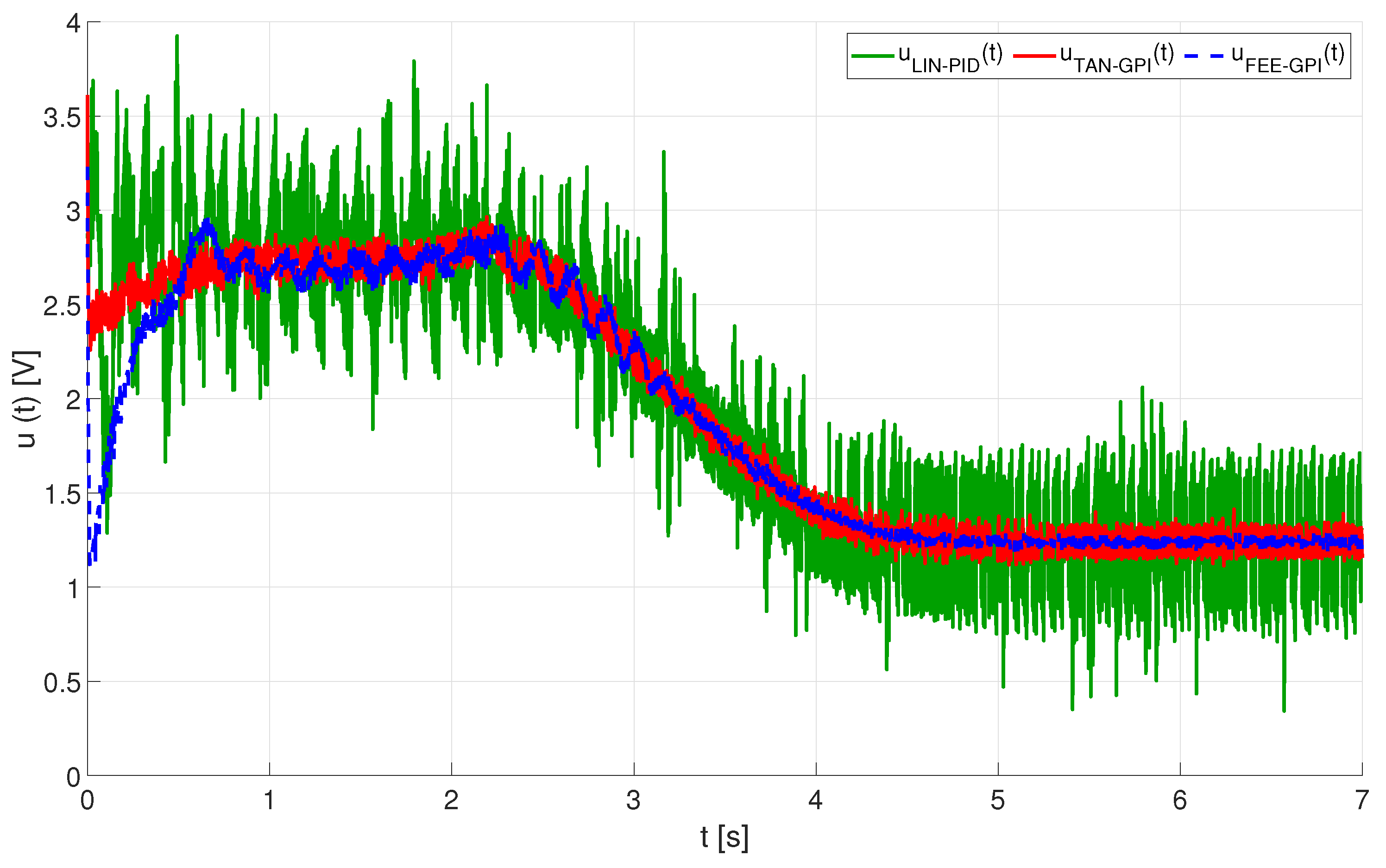
5. Experimental Results on the Magnetic Levitation Platform

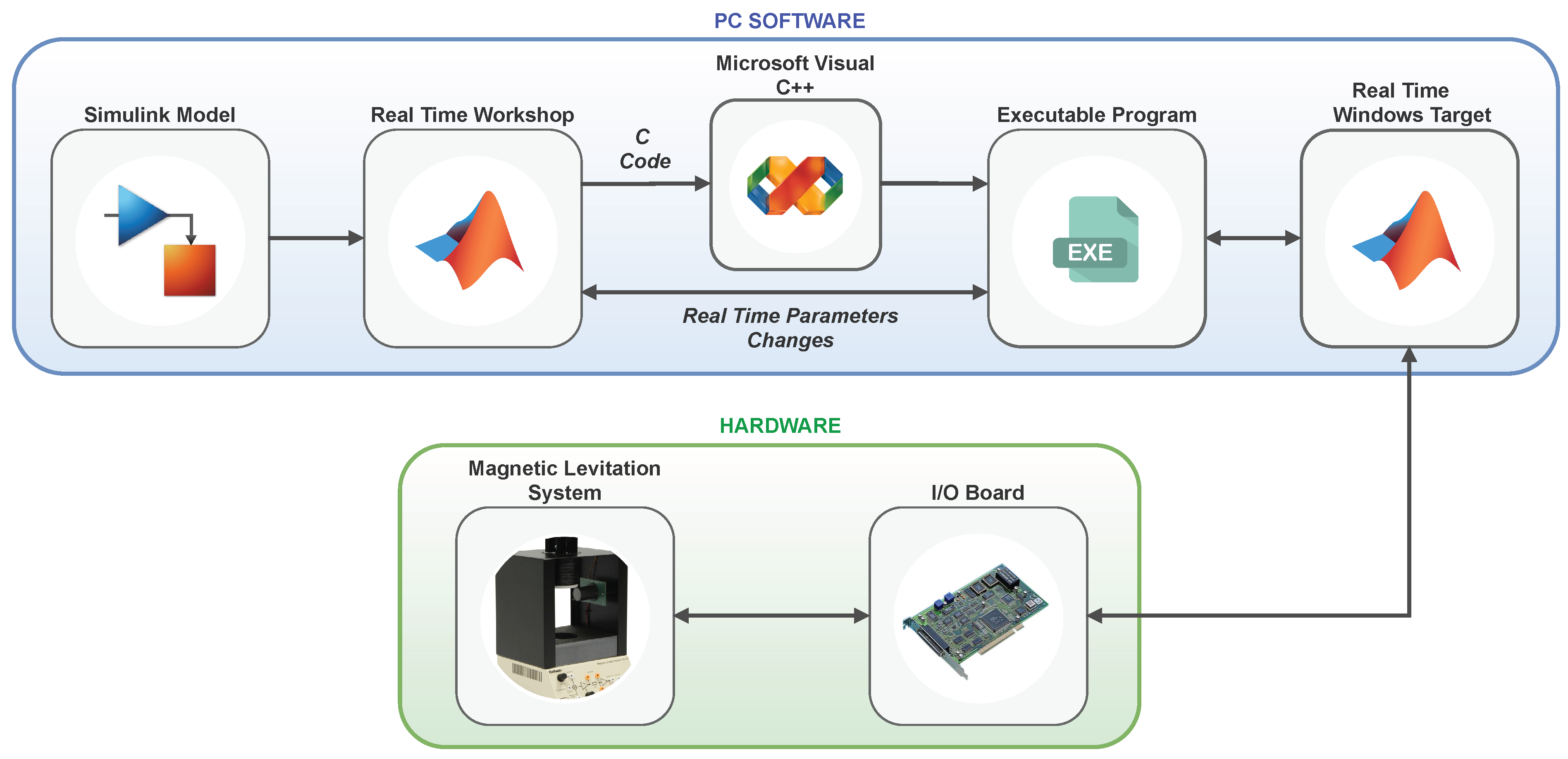
5.1. Schematics of the Experimental Implementation of the Controller

Figure 13 shows the magnetic levitation system (Maglev) employed in the trials. This attraction-type levitation system is a very challenging plant owing to its strong open-loop instability and inherent non-linearities. The structure of the magnetic levitation system comprised the mechanical unit (Feedback model 33-210), which is numbered 1 in Figure 13, and an Analogue Control Interface (Feedback model 33-301), which is numbered 2 in Figure 13 and which transferred control signals back and forth between the PC and Maglev. The Mechanical Unit and the Control Interface were linked to each other by means of lead connections. The Advantech PCI1711I/O Card (component 3 in Figure 13) was, moreover, inserted into a PCI computer slot, and was connected to the Feedback SCSI Adapter Box (4 in Figure 13) by employing the SCSI cable. The control law utilised on the PC (which operated in a Windows environment) employed Mathworks Inc. software tools, some of which are MATLAB, Simulink, Control Toolbox, Real Time Workshop (RTW), Real Time Windows Target (RTWT) and Visual C++ Professional.

Figure 14 also shows the steps required in order to attain the executable file from the control law model. MATLAB functioned as the application host environment, in which the other Mathworks products ran, and provided extensive state-of-the-art control design toolboxes. The well–structured user-friendly graphical interface for the implementation of the control law was provided by Simulink, while Real Time Workshop automatically buildt a C++ source programme from the Simulink Model. The code created by Real Time Workshop was compiled and linked using C++ compiler in order to produce an executable programme. Real Time Windows Target communicated with the executable programme, which acted as the Control Programme and interfaced with the hardware device by means of the I/O Board. The two way data or signal flow to and from the model (now an executable programme), and to and from the I/O Board was controlled by Real Time Windows Target. This approach had the advantage that the designer needed only model the process using the graphics tools available in Simulink, and did not have to worry about the communication mechanics to and from the control platform.

5.2. Results of the Experiments

In order to verify the efficiency of the proposed GPI controller in real conditions, we experimented the proposed control in a real laboratory Maglev platform, which is depicted in Figure 13. The control strategy was implemented on the Matlab-Simulink software. Details concerning the parameters of the magnetic levitation system, along with the control parameters used and the reference trajectory to be tracked, were provided in Section 4. Finally, the sampling time used in the trials was set at 0.002 s in accordance with Haykin’s condition [27]. The experimental results of the proposed GPI controller are shown in Figure 15, Figure 16 and Figure 17, again in comparison with the standard PID controller and the feedforward-GPI.

Figure 15 represents the reference trajectories for the magnetic ball and the actual trajectory followed by the ball in the MLS as a result of the action of the three controllers. Note that the proposed scheme achieved a better stabilisation and a high accuracy when tracking the Bezier trajectory. However, the trajectory followed by the ball under the action of the PID controller or the feedforward-GPI was imprecise, with an oscillatory behaviour, which undoubtedly resulted in a worse tracking of the reference trajectory. This is also clearly shown in Figure 16, which represents the ball trajectory tracking error, i.e., the difference between the Bezier reference trajectory and that followed by the ball, and shows how the GPI controller guided the error to a neighbourhood very close to 0 and much lower than that achieved by the PID controller or the feedforward counterpart. Finally, the better performance of the GPI controller was also evident if we analysed Figure 17, which represents the control input applied to the MLS. Here, it is worth mentioning that the control effort required by the PID was much higher than the proposed GPI controller and the feedforward-GPI, the effort of which decreased as the test progressed.

Finally, to conclude the analysis of the experimental tests performed, Figure 18 illustrates the ISE, IAE and ITAE parameters previously defined in Section 4.4. The values obtained were always lower for the case of the GPI controller, with a clear difference with respect to the PID and the feedforward-GPI in the case of the IAE and ITAE metrics. Hence, the superiority of the proposed GPI control over the traditional controller and the previous GPI version was once again evident.

6. Conclusions

This paper illustrates the exploitation of the local flatness property and the use of GPI controllers based on tangent linearisation within the context of the stabilisation and trajectory tracking problems for nonlinear unstable, magnetic levitation systems. The fact that the tangent linearisation of the magnetic levitation system around an arbitrary unstable equilibrium point is locally controllable implies that the system is also locally flat. This allows the design of a robust GPI control, which includes extra integration terms of the incremental tracking output error with the aim of rejecting an ultra-local internal model of the lumped additive disturbance input of finite low order. The proposed GPI controller guarantees locally exponentially asymptotic stability for the stabilisation problem and practical and local stability as regards the solution to the incremental tracking output error.

Simulations were carried out, during which the robustness of the proposed GPI control was evaluated with regard to large initial errors, the ignored non-linearities in the linearisation process, the presence of parametric uncertainties and the measurement noises. A comparison between the proposed controller, a standard PID controller and a feedforward-GPI controller [19] was performed by means of performance measurements. The results indicate that the proposed robust GPI control has a better dynamic response than the the other two controllers and show an improved performance in terms of ISE, IAE and ITAE. Experiments with the proposed GPI controller were carried out using a real laboratory magnetic levitation system, and the results obtained showed that the feedback regulation scheme performed extremely well in the stabilisation and trajectory tracking tasks, again outperforming the performance offered by a traditional PID controller or the feedforward-GPI version. Using the parameters ISE, IAE and ITAE, the superiority of the proposed scheme was also numerically evidenced.

Finally, the proposed feedback scheme could be combined with other control and estimation techniques, such as algebraic derivative estimation [36] or online algebraic filtering [37], among others, which have been very useful as regards obtaining signals with a very small noise component, thus allowing the achievement of new robust control strategies for magnetic levitation systems. These will be the topics of our future research.

References

1. Lilienkamp, K.A. Low-cost magnetic levitation project kits for teaching feedback system design. In Proceedings of the 2004 American Control Conference, Boston, MA, USA, 30 June–2 July 2004; Volume 2, pp. 1308–1313. [Google Scholar] [CrossRef]
2. Ono, M.; Koga, S.; Ohtsuki, H. Japan’s superconducting Maglev train. IEEE Instrum. Meas. Mag. 2002, 5, 9–15. [Google Scholar] [CrossRef]
3. Powell, J.; Maise, G.; Paniagua, J.; Rather, J. Maglev Launch and the Next Race to Space. In Proceedings of the 2008 IEEE Aerospace Conference, Big Sky, MT, USA, 1–8 March 2008; pp. 1–20. [Google Scholar] [CrossRef]
4. Khamesee, M.B.; Kato, N.; Nomura, Y.; Nakamura, T. Design and control of a microrobotic system using magnetic levitation. IEEE/ASME Trans. Mechatron. 2002, 7, 1–14. [Google Scholar] [CrossRef]
5. Chacon, J.; Saenz, J.; Torre, L.D.l.; Diaz, J.M.; Esquembre, F. Design of a Low-Cost Air Levitation System for Teaching Control Engineering. Sensors 2017, 17, 2321. [Google Scholar] [CrossRef] [Green Version]
6. Chacón, J.; Vargas, H.; Dormido, S.; Sánchez, J. Experimental Study of Nonlinear PID Controllers in an Air Levitation System. IFAC-PapersOnLine 2018, 51, 304–309. [Google Scholar] [CrossRef]
7. Baranowski, J.; Piątek, P. Observer-based feedback for the magnetic levitation system. Trans. Inst. Meas. Control 2012, 34, 422–435. [Google Scholar] [CrossRef]
8. Yang, Z.; Kunitoshi, K.; Kanae, S.; Wada, K. Adaptive Robust Output-Feedback Control of a Magnetic Levitation System by K-Filter Approach. IEEE Trans. Ind. Electron. 2008, 55, 390–399. [Google Scholar] [CrossRef]
9. Hypiusová, M.; Rosinová, D.; Kozáková, A. Comparison of State Feedback Controllers for the Magnetic Levitation System. In Proceedings of the 2020 Cybernetics & Informatics (K&I), Velke Karlovice, Czech Republic, 29 January–1 February 2020; pp. 1–6. [Google Scholar] [CrossRef]
10. Ni, F.; Zheng, Q.; Xu, J.; Lin, G. Nonlinear Control of a Magnetic Levitation System Based on Coordinate Transformations. IEEE Access 2019, 7, 164444–164452. [Google Scholar] [CrossRef]
11. Chopade, A.S.; Khubalkar, S.W.; Junghare, A.S.; Aware, M.V.; Das, S. Design and implementation of digital fractional order PID controller using optimal pole-zero approximation method for magnetic levitation system. IEEE/CAA J. Autom. Sin. 2018, 5, 977–989. [Google Scholar] [CrossRef]
12. Green, S.A.; Craig, K.C. Robust, Digital, Nonlinear Control of Magnetic-Levitation Systems. J. Dyn. Syst. Meas. Control 1998, 120, 488–495. [Google Scholar] [CrossRef]
13. Yang, Z.; Tsubakihara, H.; Kanae, S.; Wada, K.; Su, C. A Novel Robust Nonlinear Motion Controller with Disturbance Observer. IEEE Trans. Control Syst. Technol. 2008, 16, 137–147. [Google Scholar] [CrossRef]
14. Bidikli, B. An observer-based adaptive control design for the maglev system. Trans. Inst. Meas. Control 2020, 42, 2771–2786. [Google Scholar] [CrossRef]
15. Zhang, Y.; Xian, B.; Ma, S. Continuous Robust Tracking Control for Magnetic Levitation System with Unidirectional Input Constraint. IEEE Trans. Ind. Electron. 2015, 62, 5971–5980. [Google Scholar] [CrossRef]
16. Tepljakov, A.; Alagoz, B.B.; Gonzalez, E.; Petlenkov, E.; Yeroglu, C. Model Reference Adaptive Control Scheme for Retuning Method-Based Fractional-Order PID Control with Disturbance Rejection Applied to Closed-Loop Control of a Magnetic Levitation System. J. Circuits Syst. Comput. 2018, 27, 1850176. [Google Scholar] [CrossRef]
17. Alimohammadi, H.; Alagoz, B.B.; Tepljakov, A.; Vassiljeva, K.; Petlenkov, E. A NARX Model Reference Adaptive Control Scheme: Improved Disturbance Rejection Fractional-Order PID Control of an Experimental Magnetic Levitation System. Algorithms 2020, 13, 201. [Google Scholar] [CrossRef]
18. Morales, R.; Sira-Ramírez, H.; Feliu, V. Adaptive control based on fast online algebraic identification and GPI control for magnetic levitation systems with time-varying input gain. Int. J. Control 2014, 87, 1604–1621. [Google Scholar] [CrossRef]
19. Morales, R.; Sira-Ramírez, H. Trajectory tracking for the magnetic ball levitation system via exact feedforward linearisation and GPI control. Int. J. Control 2010, 83, 1155–1166. [Google Scholar] [CrossRef]
20. Morales, R.; Feliu, V.; Sira-Ramirez, H. Nonlinear Control for Magnetic Levitation Systems Based on Fast Online Algebraic Identification of the Input Gain. IEEE Trans. Control Syst. Technol. 2011, 19, 757–771. [Google Scholar] [CrossRef]
21. Levine, J. Analysis and Control of Nonlinear Systems. A Flatness-Based Approach; Springer Science & Business Media: Berlin, Germany, 2009. [Google Scholar] [CrossRef]
22. Sira-Ramírez, H.; Agrawal, S. Differentially Flat Systems; Automation and Control Engineering; CRC Press: Boca Raton, FL, USA, 2018. [Google Scholar]
23. Fliess, M.; Lévine, J.; Martin, P.; Rouchon, P. Flatness and defect of nonlinear systems: Introductory theory and examples. Int. J. Control 1995, 61, 1327–1361. [Google Scholar] [CrossRef] [Green Version]
24. Rouchon, P.; Fliess, M.; Levine, J.; Martin, P. Flatness, motion planning and trailer systems. In Proceedings of the 32nd IEEE Conference on Decision and Control, San Antonio, TX, USA, 15–17 December 1993; Volume 3, pp. 2700–2705. [Google Scholar] [CrossRef] [Green Version]
25. Levine, J. Analysis and Control of Nonlinear Systems; Springer: Berlin/Heidelberg, Germany, 2009. [Google Scholar] [CrossRef]
26. Hurley, W.G.; Wolfle, W.H. Electromagnetic design of a magnetic suspension system. IEEE Trans. Educ. 1997, 40, 124–130. [Google Scholar] [CrossRef]
27. Haykin, S. A unified treatment of recursive digital filtering. IEEE Trans. Autom. Control 1972, 17, 113–116. [Google Scholar] [CrossRef]
28. Åström, K.; Hägglund, T. Advanced PID Control; ISA—The Instrumentation, Systems and Automation Society: Pittsburgh, PA, USA, 2006. [Google Scholar]
29. Riggs, J.B.; Karim, M.N. Chemical and Bio-Process Control; International Edition, 3/E; Pearson: New York, NY, USA, 2008. [Google Scholar]
30. Horno, L.D.; Somolinos, J.A.; Segura, E.; Morales, R. A New Proposal for the Closed-Loop Orientation Control of a Windfloat Turbine System. J. Mar. Sci. Eng. 2021, 9, 26. [Google Scholar] [CrossRef]
31. Schultz, W.C.; Rideout, V.C. Control system performance measures: Past, present, and future. IRE Trans. Autom. Control 1961, AC-6, 22–35. [Google Scholar] [CrossRef]
32. Nagrath, I.J.; Gopal, M. Control Systems Engineering; New Age International Publishers: New Delhi, India, 2007. [Google Scholar]
33. Panduro, R.; Segura, E.; Belmonte, L.M.; Fernández-Caballero, A.; Novais, P.; Benet, J.; Morales, R. Intelligent trajectory planner and generalised proportional integral control for two carts equipped with a red-green-blue depth sensor on a circular rail. Integr. Comput. Aided Eng. 2020, 27, 267–285. [Google Scholar] [CrossRef]
34. Zurita-Bustamante, E.W.; Linares-Flores, J.; Guzman-Ramirez, E.; Sira-Ramirez, H. A Comparison Between the GPI and PID Controllers for the Stabilization of a DC–DC “Buck” Converter: A Field Programmable Gate Array Implementation. IEEE Trans. Ind. Electron. 2011, 58, 5251–5262. [Google Scholar] [CrossRef]
35. Belmonte, L.M.; Morales, R.; Fernández-Caballero, A.; Somolinos, J.A. A Tandem Active Disturbance Rejection Control for a Laboratory Helicopter With Variable-Speed Rotors. IEEE Trans. Ind. Electron. 2016, 63, 6395–6406. [Google Scholar] [CrossRef]
36. Morales, R.; Somolinos, J.; Sira-Ramírez, H. Control of a DC motor using algebraic derivative estimation with real time experiments. Measurement 2014, 47, 401–417. [Google Scholar] [CrossRef] [Green Version]
37. Morales, R.; Segura, E.; Somolinos, J.; Núñez, L.; Sira-Ramírez, H. Online signal filtering based on the algebraic method and its experimental validation. Mech. Syst. Signal Process. 2016, 66–67, 374–387. [Google Scholar] [CrossRef]
Figure 1. Diagram of Magnetic Levitation System.
Mathematics 09 01424 g001
Figure 2. GPI control scheme.
Mathematics 09 01424 g002
Figure 3. Evolution of the tracking trajectory of the magnetic ball, y * ( t ) [ m ] vs. y ( t ) [ m ] , nominal case (Test 1).
Mathematics 09 01424 g003
Figure 4. Evolution of tracking error trajectory of the magnetic ball, e ( t ) = y ( t ) y * ( t ) [ m ] , nominal case (Test 1).
Mathematics 09 01424 g004
Figure 5. Control input of the magnetic levitation system, u ( t ) [ V ] , nominal case (Test 1).
Mathematics 09 01424 g005
Figure 6. Evolution of the tracking trajectory of the magnetic ball, y * ( t ) [ m ] vs. y ( t ) [ m ] , with measurement noises at the control input and the output of the MLS (Test 2).
Mathematics 09 01424 g006
Figure 7. Evolution of tracking error trajectory of the magnetic ball, e ( t ) = y ( t ) y * ( t ) [ m ] , with measurement noises at the control input and the output of the MLS (Test 2).
Mathematics 09 01424 g007
Figure 8. Control input of the magnetic levitation system, u ( t ) [ V ] , with measurement noise at the control input and the output of the MLS (Test 2).
Mathematics 09 01424 g008
Figure 9. Evolution of the tracking trajectory of the magnetic ball, y * ( t ) [ m ] vs. y ( t ) [ m ] , with measurement noises and controller gain mismatches (Test 3).
Mathematics 09 01424 g009
Figure 10. Evolution of tracking error trajectory of the magnetic ball, e ( t ) = y ( t ) y * ( t ) [ m ] , with measurement noises and controller gain mismatches (Test 3).
Mathematics 09 01424 g010
Figure 11. Control input of the magnetic levitation system, u ( t ) [ V ] , with measurement noises and controller gain mismatches (Test 3).
Mathematics 09 01424 g011
Figure 12. Performance of the control methods in different numerical simulations.
Mathematics 09 01424 g012
Figure 13. Experimental platform.
Mathematics 09 01424 g013
Figure 14. Control System Development Flow Diagram.
Mathematics 09 01424 g014
Figure 15. Evolution of the tracking trajectory of the magnetic ball, y * ( t ) [ m ] vs. y ( t ) [ m ] , (Experimental Test).
Mathematics 09 01424 g015
Figure 16. Evolution of tracking error trajectory of the magnetic ball, e ( t ) = y ( t ) y * ( t ) [ m ] , (Experimental Test).
Mathematics 09 01424 g016
Figure 17. Control input of the magnetic levitation system, u ( t ) [ V ] , (Experimental Test).
Mathematics 09 01424 g017
Figure 18. Performance of the control methods in experimental trials.
Mathematics 09 01424 g018
Publisher’s Note: MDPI stays neutral with regard to jurisdictional claims in published maps and institutional affiliations.