Abstract
In this paper, a method for detecting synergistic effects of the interaction of elements in multi-element stochastic systems of separate redundancy, multi-server queuing, and statistical estimates of nonlinear recurrent relations parameters has been developed. The detected effects are quite strong and manifest themselves even with rough estimates. This allows studying them with mathematical methods of relatively low complexity and thereby expand the set of possible applications. These methods are based on special techniques of the structural analysis of multi-element stochastic models in combination with majorant asymptotic estimates of their performance indicators. They allow moving to more accurate and rather economical numerical calculations, as they indicate in which direction it is most convenient to perform these calculations.
MSC:
60J28
1. Introduction
Questions of composition and decomposition in multi-element stochastic systems are relevant for solving a number of problems. These include paralleling of algorithms and programs, modeling of supercomputers, the Internet, computer networks, mobile telephone communication systems, development of software packages for modeling catastrophic events in complex systems, design and improvement of technological and economic processes, and so on.
The term “synergy” (the result of the interaction of many elements of the system) originated in statistical physics, but recently it has been used by specialists from other fields: economics, biology, engineering, etc. Furthermore, research in these areas no longer leads to microscopic, but to phenomenological considerations. Here are some examples, taken from science history and devoting the detection of synergistic effects in complex systems, which have been obtained by famous researchers in their objective areas, using observation and mathematical intuition.
The economist A. Smith investigated the transition from shop production to manufacturing on the example of the production of safety pins. In the workshop method, the pin was made entirely by one master, performing all the operations sequentially. In manufacturing, each operation was performed by a separate master, which significantly increased labor productivity.
The physiologist I.P. Pavlov discovered the conditioned reflex by detecting feedback in the nervous system of the body. Stochastic feedback theory was developed by N. Wiener. A detailed study of the conditioned reflex led to the creation by P.K. Anokhin of the concept of a functional system that is urgently formed in the body when it is necessary to achieve the desired result and quickly disintegrates after it is achieved. N. Wiener and P.K. Anokhin collaborated in the development of this scientific direction, actively discussing the possibilities of mathematical methods in this area.
The physicist E. Rutherford discovered the atomic nucleus and proposed to P.L. Kapitsa to create an installation for the effect of a strong magnetic field on the atomic nucleus. Long-running installations were melted under the influence of a strong magnetic field. P.L. Kapitsa constructed an installation that creates a strong magnetic field for a short time, which turned out to be long enough for the processes occurring in the atomic nucleus.
Synergistic effects are a source of explicit dependencies between the characteristics of the system against the background of sufficiently large random perturbations. To study them, it was necessary to develop special techniques based on the structural analysis of multi-element stochastic models in combination with majorant asymptotic estimates of their performance indicators. This, in turn, required new techniques for working with statistical data, as well as skills in using the limit theorems of probability theory and the accompanying asymptotic expansions and estimates.
According to the author, many works on the analysis of complex multi-element systems require at the initial stage the construction of simpler models that allow you to determine the main performance indicators and the main parameters with which you can influence these indicators. For this purpose, it is very convenient to build procedures for comparing systems with different (alternative) structures to study their effectiveness with a large number of elements, with a large load, etc. For this purpose, schemes and/or modes of complex systems, computational algorithms, etc. can be used as objects of comparison. At the same time, at the initial stage of the study, a reasonable proportion should be observed between the accuracy of the calculations, which may be relatively small; the complexity of the calculations, which also should not be large; and the significance of the obtained results, which should be sufficiently large. Comparing systems with an alternative structures allows us to take these requirements into account, as with an increase in the number of elements, the differences between systems with an alternative structures are quite large.
The first author’s works, devoted to the study of synergistic effects, are analytical generalizations of the results of numerical and field experiments conducted by his colleagues in the modeling of telecommunications systems, container terminals, etc. In this connection, it should be remembered that in hydrodynamics, nonlinear soliton waves were also first discovered in the course of numerical experiments, and then their analytical theory was constructed. The use of computational experiments allows to obtain more accurate estimates of the synergistic effects. This can be used when working with models used in the programs “digital economy”, “smart city”, when modeling remote modes of operation that have become popular, on-line conferences, when using smart phones, etc. Currently, new information technologies are rapidly entering our life and their research helps us to adapt to them and to adapt these technologies themselves to the needs of potential users (for example, the use of smart phones by aged users). Nevertheless, analytical research helps to determine the direction of such research and to carry them out. In a sense, this avoids very complex structural optimization problems, a significant part of which are NP problems. Along with this, it becomes possible to use observations of complex systems, which also contributes to the study of synergistic effects in them.
In this paper, the synergistic effect is understood as a significant change in the performance indicators of a complex system when its structure changes, i.e., the connections between its elements. The complexity issues play an important role in modern systems analysis [1,2]. To reduce complexity, various techniques are used, among which the structural transformation of the system plays an important role [3,4]. This methodological technique is closely linked to the issues of the stability of a complex system [5].
Such a statement of the problem can be the comparing the reliability of separate and block reserving elements of a two-pole with unreliable edges [6]. This result is a classic in the mathematical theory of reliability and its refinement or amplification can be significant in itself. Note that the study of the reliability of two poles is widely used in various theoretical and applied studies (see, for example, in [7,8,9,10], etc. However, such a comparative analysis made in the monograph [6] of Barlow and Proshan did not develop in subsequent works, while the synergistic effects identified in this paper were very significant.
The peculiarity of this task is the use of probabilistic models, which, at first glance, complicate the task. This transition requires the selection of a new performance indicator—the required amount of reserve, which reflects the content of the reservation procedure and the novelty of the proposed approach. On the other hand, it is also necessary to construct sufficiently weak (logarithmic) dependencies of the so-introduced indicator on a number of the scheme elements. When selecting a new reserve efficiency indicator, its analogy with probabilistic metrics [11] is used. Therefore, the results obtained in this section are new, original, and significant.
Another problem considered in this paper and connected with synergistic effects appeared at the ITMM 2018 and ITMM 2020 conferences, when discussing the multi-server model of the RQ queuing system [12,13,14]. The Conference ITMM 2018 was held in conjunction with 12th International Workshop on Retrial Queues (RQ) and Related Topics with a wide representation of queuing theory researchers from Russia, India, Bulgaria, the Netherlands, and other countries. A good source of recent works on this topic is a collection of articles on RQ systems [15].
The RQ queuing system is a system in which a customer received in the presence of busy servers is not rejected, but is sent to the so-called orbit, from where it is extracted in accordance with some protocol for queuing, when one of the servers is released. A.N. Dudin remarked that it is most often assumed Poisson input flow to such a system. However, this requirement is not met because there is a dependence and even a long range dependence between the random variables, characterizing numbers of arrived customers in disjoint time intervals. Moreover, despite the large number of analytical results in which the distributions in RQ systems are calculated in formula form, their use for numerical calculations is difficult due to the high complexity of such calculations, especially for multi-server RQ systems.
The novelty of the proposed approach is that instead of a stationary distribution of the process describing a multi-server RQ system, the probability of customers appearing in the orbit of this system for a fixed period of time is investigated and the convergence of this indicator to zero is established when the number of channels proportional to the intensity of the input flow tends to infinity. Secondly, with an increase in the number of servers, even in a system with a Poisson input flow and exponentially distributed service times, the computational complexity of the problem of calculating the limit distribution in an RQ system increases quite strongly.
Thus, a new problem arises for calculating the RQ queuing system with a large number of servers and a non-Poisson input flow. Using asymptotic theorems for multichannel queuing systems, it is possible, on the contrary, to simplify the problem of analyzing RQ systems. For this purpose, it is convenient to use limit theorems based on topological concepts of convergence in the space of random processes defined on a finite time interval [16]. The significance of this approach lies in the broad scope of its application and in the ability to circumvent the computational complexity of the problem by reducing it to the limit theorems of probability theory.
A continuation of the study of multi-server queuing systems in this paper is the analysis of a system with failures. This system arises when modeling modern data transmission networks (of fifth generation), formulated by leading Russian specialists in the mathematical theory of communication [17]. This task is quite important and leading Russian specialists in modeling of transmission networks Samouylov K.E. and Gaidamaka Yu.V. even organized a seminar with the author’s participation to find alternative approaches to this problem solution with publishing of obtained results [18]. The solution to this problem is based on the recently installed a synergistic effect in multi-server queuing system with failures, when the stationary probability of failure tends to zero as the number of servers and proportionally the input flow intensity tend to infinity. Moreover, the obtained asymptotic results were quite accurate.
This study is based on the classical Erlangian model of loss multi-server system (see, for example, in [19,20]). Asymptotic behaviors of the blocking probability and parameters of the Equivalent Random Theory method was analyzed in [21] for the case when both the number of servers and the input flow intensity tend to infinity.
However, the inclusion in this model of the assumption that load factor equals one, the intensity of the input flow is proportional to the number of servers n, and the tendency of n to infinity allowed us to establish that the probability of failure tends to zero also. The exact asymptotic rate of this convergence is established. Moreover, when the load factor is less than one, it is possible to construct an upper estimate of the rate of convergence to zero in the form of a geometric progression. Therefore, the synergistic effect found in this paper is very strong and so can be used in the design of data transmission systems of the fifth generation.
The features of probabilistic models of complex systems discovered in this way can also be used in the estimation of their parameters. In particular, in the deterministic model of logistic growth [22] (which is very important and classical in mathematical biology), the problem of estimating the growth parameter from inaccurate observations arises and attracts specialists again and again. The solution of this problem by the method of least squares leads to quite large errors. In this paper, the unknown growth parameter is expressed in terms of the trajectory averages of the deterministic sequence of the model. In turn, the trajectory averages are estimated from observations over a sufficiently long period of time, which leads to the leveling of observation errors. These estimates are based on the use of probabilistic metrics developed in [11] and are new.
Thus, the solution of the above problems of system analysis required a combination of probabilistic and deterministic methods of system analysis, among which the methods of studying the synergistic effects arising from the structural restructuring of a complex system play a decisive role. The benefit of received results is to establish sufficiently strong dependencies of performance indicators on changes in the system structure. This approach opens up new opportunities in solving problems of structural optimization of stochastic systems: queuing, reliability, etc.
2. Separate Redundancy in a Two-Pole System
Consider m sequentially connected and independently operating elements with a failure-free probability of The probability of failure-free operation of such a chain is . Let us focus on two alternative ways to reserve this network. In the first method, n independently functioning duplicates are connected in parallel (see Figure 1).
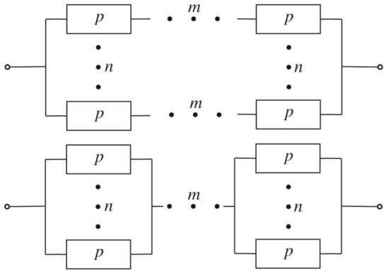
Figure 1.
n-multiple block redundancy (top), split redundancy (bottom) of a chain of length
Reliability of the network obtained in this way is In the second method, each element of the original chain is n-multiple reserved separately (see Figure 1). Reliability of the newly formed network
From the results of the monograph [6], it follows that (this inequality is valid for any bipolar). However, this inequality gives only a qualitative idea of the possibilities of separate reservation. To give a quantitative assessment, it is convenient to move from the reliability function to the required amount of reserve.
For , denote the required volume of reserve, in which the reliability exceeds To calculate the reliability of general type two-pole, it is necessary to solve an NP-complex problem. However, to compare the different ways of reserving a chain of the length it is necessary only to solve a few simple inequalities. Moreover, the results of this comparison are very contrasting and the most interesting consideration of a separate reserve may be applied to general type two-pole also. Let us denote the integer part of the real number
Proposition 1.
The following inequalities are met:
Proof.

Therefore, the second relation in Formula (1) is valid.
Table 1 demonstrates how much is greater than □
Table 1.
Meanings of for
A comparison of these relations shows that for a large chain length of m, the split-reservation scheme provides special advantages, as the lower bound, which grows as a geometric progression, is replaced by the upper logarithmic bound. Note that the upper estimate of the required reserve in the scheme of separate reservation of a sequential chain is logarithmic in m and can be easily extended to the general case.
Indeed, consider a two-pole consisting of m independently operating edges with probabilities of operation Let us construct a two-pole in which each edge of the original two-pole is a reserve of n identical elements and denote the probability of the existence of a working path from the initial to the final vertex in this two-pole.
Proposition 2.
For the value , the relation is valid
Proof.
The proof of this statement is based on the inequality This inequality follows from the fact that the reliability of an arbitrary two-pole with m independently functioning elements is not less than the reliability of a chain of m elements connected in series. Therefore, the second inequality in the formula (1) is true also. □
For an arbitrary two-pole, a logarithmic by m upper estimate of the value of the required reserve in the separate reservation scheme is performed. Note that this result is obtained using trivial inequalities and does not require calculating the reliability of which in general is an NP-problem.
Indeed, if are independent boolean random variables which describe states of two-pole elements and boolean function describes a workability of two-pole dependently on states of its elements then its reliability
Calculation of the reliability formally requires performing of arithmetical operations.
Thus, a convenient choice of the reserve efficiency indicator in the form of the required reserve volume solves two problems. It allows us to obtain a strong (logarithmic) dependence of the chosen efficiency indicator on the number of edges of the two-pole m and makes it possible to abandon the solution of the NP-problem of calculating the reliability of the two-pole.
3. RQ-Queuing Systems with a Large Number of Servers
Consider an RQ-system, i.e., a queuing system, in which, if there is a free server, the customer that has come to the system immediately begins to be served on it. If there are no free servers, then the customer is sent to the orbit, from where it can return to the newly released server in accordance with some protocol [12,14,23]. A good source for RQ systems in recent years has been Conference ITMM 2018 in Tomsk, which was held in conjunction with 12th International Workshop on Retrial Queues and Related Topics (WRQ 2018).
To solve this problem, we propose to use the theorem on the asymptotic behaviour of an n-server queuing system for In this theorem, we prove that at for the probability that on the segment in the system there will be customers going into orbit tends to zero. Already in this result, the transition from the limit distribution to the above probability is made. Moreover, this characteristic becomes a new indicator of efficiency, which is convenient to use when analyzing a multichannel RQ queuing system.
Consider the series scheme in which the characteristics of n-server queuing systems are defined by the parameter which characterizes an intensity of input flow tending to infinity. Denote a number of input flow customers arriving before the moment t, Assume that is a number of busy servers in this system at the moment is the service time of j input flow customer and is a sequence of independent and identically distributed random variables (s.i.i.d.r.v.’s) with the distribution function (d.f.) which has continuous and bounded by density All results of this section are based on ([16], Chapter II, § 1, Theorem 1):
Theorem 1.
Assume that the following conditions are true.
- (1)
- For some the equality takes place.
- (2)
- There is the function such that for the limit relations take place forso that ).
- (3)
- The sequence of random processes for C-converges to the centred Gaussian process
- (4)
- Random process where is centred Gaussian process independent with which has the covariance function and satisfies the relation
- (5)
- If the inequality is true then for any we have the relation
Here, the concept of C-convergence used in Theorem 1 is defined as follows. Denote by the space of deterministic functions on the segment with uniform metric Designate by the set of bounded functionals f defined on and continuous in the metric if and then Say that the sequence of random processes C-converges to the random process if for any functional we have that
Deterministic input flow of customer groups. Let at times in n-server RQ-queuing system come groups of customers of the size of where – i.i.d.r.v.‘s with integer values, Define the input flow by the equality where – independent of a random variable with a uniform distribution on the segment ( is the integer part of the real number d). Here and in two next models random variable has uniform distribution to ensure the proportionality t of the mathematical expectation
Theorem 2.
Suppose that, for some almost certainly and the inequality is true. Then for any the relation is valid.
Proof.
In [23] it is proved that under the conditions of this theorem,
Connecting this relation with the inequality one obtains the proof of the theorem. □
Alternating input flow. Consider a n-server RQ-queuing system, assuming Let us define the input flow to this system using the following construction. Following the works in [24,25], we define a continuous random flow defined by ON and OFF periods. Let a sequence of i.i.d.r.v’s consists of lengths of ON-periods, the sequence of i.i.d.r.v.‘s consists of the lengths of OFF-periods and these random sequences are independent. Denote and suppose that
where the function and is a slowly varying function. Let is the inverse of the function
We introduce independent r.v.‘s , which are independent of and with distributions
Then, a random sequence
generates an ON–OFF process
(here is the indicator function of a random event ). The random process is binary: if t is contained in an ON-period, if t is contained in the OFF-period and stationary, and
Denote then Let and random functions are independent copies of a random function We introduce the function specifying the alternating input flow.
Theorem 3.
If and then for any the relation is true.
The proof of Theorem 3 repeats the proof of Theorem 2 verbatim.
Erlangian input flow. Let a Poisson flow of customers with intensity Define the input flow to the n-server system described above by the equality
where is a random variable independent of with a uniform distribution on the segment , and the fixed r takes natural values. It is obvious that for any fixed the moments of single jumps of the process form an Erlangian flow. Here, the Erlangian flow is obtained from by allocation of moments with numbers that are multiples of
Theorem 4.
If then for any the relation holds.
Proof.
In [26] it is proved that Formula (2) is valid under the conditions of the theorem. Connecting it with inequality one obtains the proof of the theorem. □
The choice of the probability as an efficiency indicator allows us to apply the known theorems to the analysis of a multi server RQ-system with a fairly general protocol for the transfer of customers from orbit to the vacated server almost without additional consideration.
4. Multiserver Loss Systems
Consider n-server queuing system with a Poisson input flow of intensity and exponentially distributed service times having intensity on all n servers, This system can be considered as combining n single-server systems with input flow intensities (see Figure 2).
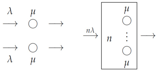
Figure 2.
n isolated systems (left), aggregated system (right). .
The number of customers in the system describes the process of death and birth with the intensities of birth and death
Let us denote the stationary probability of failure in the system for a given It is not difficult to establish that However, the combined system satisfies new relation, which characterizes the synergistic effect of such a combination.
Theorem 5.
The following limit ratio is true:
Proof.
Let consider the function The function satisfying the condition: and such that the inequalities
hold. Therefore, on the half interval there exists a single satisfying the condition and such that the inequalities hold. Let then in force [16] [Chapter 2, § 1]
Therefore, the stationary blocking probability in virtue of the integral theorems of recovery and the law of large numbers for the recovery process [1] [Chapter 9, § 4, 5] satisfies the equality
where equals From Formula (3), we obtain the inequality
This implies that
consequently
and so
Using Formula (3) and the inequality we obtain
thus it follows that Obtained above inequalities for upper and lower limits lead to the statement of Theorem 5. □
Remark 1.
In aggregated system at following relations are valid [18]:
And if then Theorem 5 gives
Similar results were obtained for Erlang‘s loss function in [27,28] but in a more complex way.
Remark 2.
In aggregated system following relations are valid [29] for —stationary mean waiting time and —stationary mean queue length:
- (1)
- If then for some the relation holds
- (2)
- If then for
Suppose that we have m independently functioning -server queuing systems with Poisson input flows of intensity In the k-th system, the customer of the input flow is served exponentially distributed time simultaneously on channels with intensity Let be a natural number and the equality holds.
We combine n copies of each of the -server systems under consideration, denoting stationary probability of failure in each of the combined systems, Using Theorem 5, it is not difficult to obtain the following limit relations
This solution allows us to distribute the total number of servers between flows so that the failure probabilities of customers of different flows tend to zero with the growth of a large parameter To solve this problem, one could use the exact multiplicative formula obtained in [17], but this would lead to significantly more complex calculations.
5. Parameter Estimation in the Logistics Growth Model
The recurrent model of logistic growth
where the parameters satisfy the conditions attracts increased attention from biologists and physicists. For this model, both practically and theoretically, it is important to evaluate the parameter b based on inaccurate observations. Due to the nonlinearity of the recurrence relation (5), the least squares method applied to the estimation of the parameter b seems somewhat unnatural, which is confirmed by numerous computational experiments that give quite large errors. It seems more natural to apply such qualitative properties of the sequence, as the existence of its limit cycle or limit distribution [30] depending on the value of b in combination with the method of probability metrics [11].
Consider an additive model for introducing errors in observations Here, is a sequence of i.i.d.r.v.’s having a distribution with mean zero and variance . We introduce the following notation
Using the results of [30], it is possible to establish that for the deterministic sequence with a given b there are limits
Indeed, say that the sequence has a limit cycle of length , if Denote then we have
so Formula (6) is true in the case, when the sequence has limit cycle.
Let be a probability measure on the -algebra of Lebesgue-measurable subsets of the segment . Let us say that is the limiting distribution of the sequence if for any Lebesgue-measurable set the equality holds where is the number of satisfying the inclusion Then, we define and prove Formula (6) as follows.
Let us take an arbitrary and put Divide the half interval into disjoint segments
Choose so that for any we have It is sufficiently simple to prove for the following inequalities
Summing these inequalities by and using the equality for m we get for the inequality
Analogously it is possible to obtain
consequently Similarly we have the relation so Formula (6) is true in the case, when the sequence has limit distribution also.
Note that formally the limits may depend on the initial state However, in the logistics growth model there is no such dependence.
We will evaluate the parameter b in two stages. First, we express b in terms of the path averages: Using the ratio
let us estimate the parameter b by the formula
As a result, the parameter b is evaluated by the formula The convergence in probability follows from the relations
The following is an illustrative example of estimating parameter b for a logistic growth model. Calculations of were performed for the case at (see Figure 3). An additive model of introducing errors was considered under the assumption that have a uniform distribution on the segment
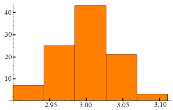
Figure 3.
Frequency histogram for .
This method can be applied to the estimation of the parameters of the Rikker model (see, for example, in [22]). Here, the Rikker model is described by recurrent relation
and observations are following: where has normal distribution with zero mean and known variation, Another application of described method is the finite-difference approximation of the system of Lorentz differential equations (see, for example, in [31]), etc.
6. Discussion
All the problems of system analysis considered in this paper are based on the choice of changes in the structure of the system, the efficiency indicator, and the computational algorithm with an assessment of its complexity. In some cases, it is possible to replace the NP-problem with a fairly simple computational procedure, abandoning the high accuracy of the resulting solution in favor of a significant change in the performance indicator. Apparently, such problems require a certain proportion between the accuracy and efficiency of the resulting solution.
The proposed approach to the study of synergistic effects in complex systems can be applied to the construction of queuing systems with a large load and a small queue, to backup systems with recovery, to insurance models and other stochastic systems. It allows you to explore and find the main parameters in such popular technologies in applications as powder metallurgy, 3-D printing, fast mixing of fuel in engines, etc. The emphasis on economical, but not highly accurate calculations, makes it possible at the initial stage to correctly select the main parameters of the analyzed systems before performing more detailed and accurate calculations. This property of the proposed approach to the analysis of complex systems can be used in programs of digital economy, smart city, etc., when at the initial stage of the study it is important to determine the main indicators of the effectiveness of a complex system.
Funding
This research received no external funding.
Institutional Review Board Statement
Not applicable.
Informed Consent Statement
Not applicable.
Data Availability Statement
Data sharing is not applicable to this article.
Acknowledgments
The author thanks Marina Osipova for her help in the design of the work.
Conflicts of Interest
The authors declare no conflict of interest.
References
- Skrimizea, E.; Haniotou, H.; Parra, C. On the complexity turn in planning: An adaptive rationale to navigate spaces and times of uncertainty. Plan. Theory 2019, 18, 122–142. [Google Scholar] [CrossRef]
- Battiston, S.; Caldarelli, G.; May, R.; Roukny, T.; Stiglitz, J. The price of complexity in financial networks. Proc. Natl. Acad. Sci. USA 2016, 113, 10031–10036. [Google Scholar] [CrossRef] [PubMed]
- Majdandzic, A.; Braunstein, L.; Curme, C.; Vodenska, I.; Levy-Carciente, S.; Eugene, S.; Havlin, S. Multiple tipping points and optimal repairing in interacting networks. Nat. Commun. 2016, 7, 1–10. [Google Scholar] [CrossRef] [PubMed]
- Lever, J.; Leemput, I.; Weinans, E.; Quax, R.; Dakos, V.; Nes, E.; Bascompte, J.; Scheffer, M. Foreseeing the future of mutualistic communities beyond collapse. Ecol. Lett. 2020, 23, 2–15. [Google Scholar] [CrossRef] [PubMed]
- Limiao, Z.; Guanwen, Z.; Daqing, L.; Hai-Jun, H.; Eugene, S.; Shlomo, H. Scale-free resilience of real traffic jams. Proc. Natl. Acad. Sci. USA 2019, 116, 8673–8678. [Google Scholar]
- Barlow, R.; Proshan, F. Mathematical Theory of Reliability; John Wiley and Sons: New York, NY, USA, 1965. [Google Scholar]
- Ryabinin, I.A. Reliability and Safety of Structurally Complex Systems; St. Petersburg University Press: Saint-Petersburg, Russia, 2007. (In Russian) [Google Scholar]
- Solojentsev, E.D. Scenario Logic and Probabilistic Management of Risk in Business and Engeneering; Springer: Berlin/Heidelberg, Germany, 2004. [Google Scholar]
- Gertsbakh, I. Statistical Reliability Theory; Marcel Dekker: New York, NY, USA, 1989. [Google Scholar]
- Rocchi, P. Reliability Is A New Science. Gnedenko Was Right; Springer: Berlin/Heidelberg, Germany, 2017. [Google Scholar]
- Zolotarev, V. Modern Theory of Summation of Random Variables; VSP: Utrecht, The Netherlands, 1997. [Google Scholar]
- Dudin, A.; Nazarov, A. On a tandem queue with retrials and losses and state dependent arrival, service and retrial rates. Int. J. Oper. Res. 2017, 29, 170–182. [Google Scholar] [CrossRef]
- Artalejo, J.; Gomez-Corral, A. Retrial Queueing Systems. A Computational Approach; Springer: Berlin/Heidelberg, Germany, 2008. [Google Scholar]
- Nazarov, A.; Moiseeva, E. Investigation of the RQ-system MMPP|M|1 by the method of asymptotic analysis in the condition of a large load. Izv. Tomsk. Polytech. Univ. 2013, 322, 19–23. (In Russian) [Google Scholar]
- Information Technologies and Mathematical Modelling-Queueing Theory and Applications. In Proceedings of the 17th International Conference, ITMM 2018, Named After A.F. Terpugov, and 12th Workshop on Retrial Queues and Related Topics, WRQ 2018, Tomsk, Russia, 10–15 September 2018; Volume 912.
- Borovkov, A. Asymptotic Methods in Queueing Theory; John Wiley and Sons: New York, NY, USA, 1984. [Google Scholar]
- Basharin, G.P.; Gaidamaka, Y.V.; Samouylov, K.E. Mathematical Theory of Teletraffic and Its Applications to the Analysis of Multiservice Communication of Next Generation Networks. Autom. Control. Comput. Sci. 2013, 47, 62–69. [Google Scholar] [CrossRef]
- Tsitsiashvili, G.S.; Osipova, M.A.; Samoulov, K.E.; Gaidamaka, Y.V. Synergetic effects in multiserver loss systems. In Proceedings of the VIII Moscow International Conference on Operations Research for the Centenary of Yu. B. Hermeyer at the Moscow State University and the VC RAS, Moscow, Russia, 17–21 October 2016; Volume I, pp. 350–355. [Google Scholar]
- Gnedenko, B.V.; Kovalenko, I.N. Introduction to Queuing Theory; Nauka: Moscow, Russia, 1966. (In Russian) [Google Scholar]
- Ivchenko, G.I.; Kashtanov, V.A.; Kovalenko, I.N. Queuing Theory; Visshaya Shkola: Moscow, Russia, 1982. (In Russian) [Google Scholar]
- Naumov, V.A. On the behavior of the parameters of the Equivalent Random Theory method at low load. In Numerical Methods and Informatics; RUDN Publisher: Moscow, Russia, 1988. (In Russian) [Google Scholar]
- Geritz, S.; Kisdi, E. On the mechanistic underpinning of discrete-time population models with complex dynamics. J. Theor. Biol. 2004, 228, 261–269. [Google Scholar] [CrossRef] [PubMed]
- Tsitsiashvili, G.; Osipova, M. Synergetic effects for number of busy servers in multiserver queuing systems. Commun. Comput. Inf. Sci. Ser. 2015, 564, 404–414. [Google Scholar]
- Heath, D.; Resnick, S.; Samorodnitsky, G. Heavy tails and long range dependence in on/off processes and associated fluid models. Math. Oper. Res. 1998, 23, 145–165. [Google Scholar] [CrossRef]
- Mikosch, T.; Resnick, S.; Rootzen, H.; Stegeman, A. Is network traffic approximated by stable Levy motion or fractional Brownian motion? Ann. Appl. Probab. 2002, 12, 23–68. [Google Scholar] [CrossRef]
- Tsitsiashvili, G.; Markova, N. Synergistic effects in a multi-channel queuing system with an Erlangian input flow. Bull. Pac. State Univ. 2015, 4, 17–22. (In Russian) [Google Scholar]
- Jagerman, D.L. Some Properties of the Erlang Loss Function. Bell Syst. Tech. J. 1974, 53, 525–551. [Google Scholar] [CrossRef]
- Mitra, D.; Weiss, A. The Transient Behavior in Erlang’s Model for Large Trunk Groups and Various Traffic Conditions. Proc. 1988 Int. Teletraffic Congr. 1988, 26, 223. [Google Scholar] [CrossRef][Green Version]
- Tsitsiashvili, G.S.; Osipova, M.A. Phase Transitions in Multiserver Queuing Systems. Inf. Technol. Math. Model. Queueing Theory Appl. 2016, 638, 341–353. [Google Scholar]
- Sharkovskiy, A.; Sharkovskiy, A.N. Difference Equations and Population Dynamics. Preprint 82.18; Institute of mathematics of the Academy of Sciences of the Ukrainian SSR: Kiev, Ukraine, 1982. (In Russian) [Google Scholar]
- Leonov, G.; Kuznetsov, N.; Korzhemanova, N.; Kusakin, D. Lyapunov dimension formula for the global attractor of the Lorenz system. Commun. Nonlinear Sci. Numer. Simul. 2016, 41, 84–103. [Google Scholar] [CrossRef]
Publisher’s Note: MDPI stays neutral with regard to jurisdictional claims in published maps and institutional affiliations. |
© 2021 by the author. Licensee MDPI, Basel, Switzerland. This article is an open access article distributed under the terms and conditions of the Creative Commons Attribution (CC BY) license (https://creativecommons.org/licenses/by/4.0/).