Oversampling Errors in Multimodal Medical Imaging Are Due to the Gibbs Effect

Abstract

To analyze multimodal three-dimensional medical images, interpolation is required for resampling which—unavoidably—introduces an interpolation error. In this work we describe the interpolation method used for imaging and neuroimaging and we characterize the Gibbs effect occurring when using such methods. In the experimental section we consider three segmented three-dimensional images resampled with three different neuroimaging software tools for comparing undersampling and oversampling strategies and to identify where the oversampling error lies. The experimental results indicate that undersampling to the lowest image size is advantageous in terms of mean value per segment errors and that the oversampling error is larger where the gradient is steeper, showing a Gibbs effect.

1. Introduction

In the context of multimodal medical imaging [1,2,3], image data of the same physical body are obtained from different imaging systems. The resulting images have different geometrical resolutions in terms of Full Width at Half Maximum (FWHM) [4] and by consequence different samplings of the same Field Of View (FOV). In many cases, two types of image sources are involved, producing:

• one (or more) morphological, high-resolution image, usually obtained by Computed Tomography (CT) or by Magnetic resonance Imaging (MRI);
• one (or more) functional, low-resolution image. A functional image is typically obtained by Single Photon Emission Computed Tomography (SPECT), Positron Emission Tomography (PET) [3], functional MRI (fMRI) [5] or by emerging systems as Magnetic Particle Imaging (MPI) [6].

Thanks to their high spatial resolution, morphological images can be used for identifying different structures of the physical body under examination through segmentation. In order to estimate the mean activity (or any other statistical moment) of the functional images inside each of the segments or Volumes of Interest (VOIs), it is mandatory that the segmentation and the functional images have the same size. This can be achieved either by oversampling the functional image to reach the same resolution of the morphological reference or by undersampling the segmentation image [7,8]. Despite what common sense may suggest, the latter is preferable, due to the bigger interpolation errors occurring in oversampling. This represents a paradox (we will later refer to this effect as the resampling paradox), but also a big waste of time since an accurate segmentation image at high resolution (in the case of the human brain) is obtained typically after 10–20 h of manual work or 3–10 h of automatic segmentation pipelines [9].

In this paper we describe the interpolation methods used in imaging and medical imaging, focusing on the Gibbs effect [6,10,11,12]. The Gibbs effect results in an interpolation error due to a discontinuity and consists in of non-physical oscillations of higher amplitude around the discontinuity. We found a pointwise error bound for the proposed interpolation methods that does not vanish in the proximity of the point of discontinuity as the number of samples increases and that is larger in the intervals of sampling points closer to the discontinuity.

We then consider three of the most used software suites in neuroimaging performing undersampling and oversampling of three different test images. The results confirm the resampling paradox and point out that the oversampling interpolation errors are due to the Gibbs effect as the voxelwise error is mostly concentrated around the borders of the VOIs, where most of the discontinuities lie.

The authors of this paper refer to their experience in the field of PET/MRI neuroimaging [13], but the analysis and conclusions are applicable for any multimodal image setting and any scanned physical body.

The paper is organized as follows. The next section is dedicated to mathematical formulations and preliminary definitions, in which we mention some results that will be useful to understand the experimental settings and the error measures. Section three is dedicated to interpolation methods in imaging along with error estimations related to Gibbs effect. In the “Materials and Methods” section we introduce and shortly describe the three test images used in experiments, the tools used to perform undersampling and oversampling, the error measures defined for comparing undersampling versus oversampling and last the measures defined for detecting the oversampling error spatial location. Results and some explanatory comments are presented in Section 4 and Section 5. This work does not propose a method to reduce oversampling errors. However, in Section 6 we indicate possible manners of overcoming the interpolation errors issues analyzed in this paper as well as with some recent findings which have shown their efficiency in preventing the Gibbs effect.

2. Preliminaries and Definitions

2.1. The Gibbs Effect

The Gibbs effect is the non-physical oscillation generated when a discontinuous function is approximated by a truncated Fourier series [10,14]. This effect appears also in interpolation and does not vanish as the number of samples increases, but the undershoots and overshoots tend to remain stable. The overshoots have higher intensity around the borders of the discontinuities and tend to vanish as the border becomes more distant.

The Gibbs phenomenon appears everywhere in signal processing; in MRI it is also referred to as the “ringing effect” (or ringing artifact) [11,12,15] for the wave-like oscillation appearing radially around the borders of the image discontinuities that are observed in image reconstruction and image resampling.

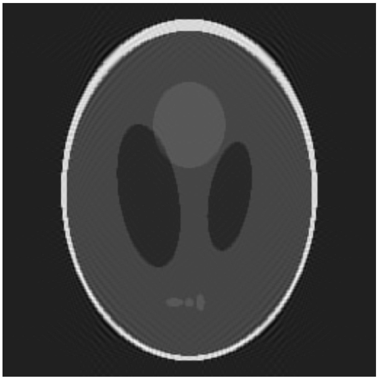
In Figure 1 it is possible to observe a simple example of Gibbs effect on the Heaviside step function; both in Truncated Fourier approximation and interpolation, oscillations not present in the original signal appear around the discontinuity, gradually mitigating their amplitude as the distance from the discontinuity increases. In Figure 2 an example of ringing effect is given using a phantom image.

2.2. An Image and Its Sampling

A 3-dimensional image can be defined as a trivariatefunction [16]

$$f:\mathsf{\Omega }\subset {\mathbb{R}}^3\to \mathbb{R}$$

(1)

where the domain $\mathsf{\Omega }$ is called Field of View (FOV) and is a rectangular parallelepiped $\mathsf{\Omega }=[a_1,b_1]\times [a_2,b_2]\times [a_3,b_3]$.

A raster image is obtained by sampling an image f on $\mathsf{\Omega }$ with a regular and equispaced three-dimensional grid $X=\left\{{\mathit{x}}_{ijk}\right\}$ of cardinality $I\times J\times K$, i.e.,

$${\mathit{x}}_{ijk}=\left(x_i,y_j,z_k\right)=\left((b_1-a_1)\frac{i-1}{I-1}+a_1,(b_2-a_2)\frac{j-1}{J-1}+a_2,(b_3-a_3)\frac{k-1}{K-1}+a_3\right)$$

(2)

with $i=1,\dots ,I,j=1,\dots ,J,k=1,\dots ,K.$

The intensity values of the raster image are stored in an array ${F=f|}_X$ of size $I\times J\times K$

$$F_{ijk}=f\left({\mathit{x}}_{ijk}\right).$$

(3)

The sampling grid is usually not stored in a file to save disk space and kept implicit.

2.3. Resampling an Image

Resampling an image means to compute it over another regular and equispaced grid $\tilde{X}$ (called evaluation grid). We refer to undersampling if $\tilde{X}$ has a lower cardinality than X, oversampling in the opposite case. Being the exact function f not known in general, to perform resampling it is necessary to compute the interpolant $\mathcal{P}f$ of the image intensity values on the known grid X over the evaluation grid $\tilde{X}$. This means, once chosen, a basis $\mathcal{B}=\left\{B_{ijk}\left(·\right)\right\}$ defines an interpolating function

$$\mathcal{P}f:\mathsf{\Omega }\subset {\mathbb{R}}^3\to \mathbb{R}$$

(4)

$$\mathcal{P}f\left(·\right)=\sum _{ijk}{c}_{ijk}{B}_{ijk}\left(·\right)$$

(5)

with $c_{ijk}$ coefficients such that the interpolation conditions

$$\mathcal{P}f\left({\mathit{x}}_{ijk}\right)=f\left({\mathit{x}}_{ijk}\right)$$

(6)

are fulfilled. At last, the resampled image is computed as the array ${\mathcal{P}f|}_{\tilde{X}}$.

Interpolation methods used in neuroimaging will be discussed in detail in the next section.

2.4. Boolean Images and Morphological Operators

A Boolean image is an image sampled over a grid as in Equation (3), but with all Boolean entries, i.e.,

$$M\in {\{0,1\}}^{I\times J\times K};$$

(7)

a Boolean image can be represented equivalently by the set of its true-valued indices

$$\mathcal{I}\left(M\right):=\left\{(i,j,k)\right|M_{ijk}=1\}\subset {\mathbb{Z}}^3.$$

(8)

This representation allows one to make some definitions (cf e.g., [17]). Given $M\in {\{0,1\}}^{I\times J\times K}$ a Boolean image, $I=\mathcal{I}\left(M\right)$ its index representation, and and image $F\in {\mathbb{R}}^{I\times J\times K}$ sampled over the same grid, we can define:

• the volume of M, as the cardinality of the corresponding index representation

  $$\mathrm{Vol}\left(M\right)=\left|\mathcal{I}\right(M\left)\right|$$

  (9)
• the restriction of F to M as the array of the values of F in the voxels where M is equal to one

  $$F\left[M\right]:=\left\{F_{ijk}\right|(i,j,k)\in \mathcal{I}\left(M\right)\}$$

  (10)
• the shift by a vector $v\in {\mathbb{Z}}^3$

  $$I_v=\{a+v|a\in I\}$$
• the dilation by a structuring element $H\subset {\mathbb{Z}}^3$

  $$I\oplus H=\bigcup _{h\in H}{I}_h$$

  (11)
• the erosion by a structuring element $M\subset {\mathbb{Z}}^3$

  $$I\ominus H=\bigcap _{h\in H}{I}_{-h}$$

  (12)

The structuring element used in this work is the three-dimensional cross

$$H=\left\{\right(0,0,0),(1,0,0),(-1,0,0),(0,1,0),(0,-1,0),(0,0,1),(0,0,-1\left)\right\}.$$

Intuitively, the dilation of a Boolean image A is a Boolean image returning one if any of the surrounding voxel of A is one, zero otherwise; on the other side the erosion returns one if all the surrounding voxels are one, zero otherwise.

2.5. Segmentation of an Image

A segmentation of an image means partitioning the FOV $\mathsf{\Omega }$ into non-overlapping sets (cf, e.g., [18]) called VOIs (Volumes Of Interest) from now on

$$\mathsf{\Omega }=\bigcup _{p=0}^n{\mathsf{\Gamma }}_p\mathrm{such}\mathrm{that}{\mathsf{\Gamma }}_p\cap {\mathsf{\Gamma }}_q=\varnothing \forall p\ne q=0,\dots ,n.$$

(13)

For each ${\mathsf{\Gamma }}_p$ we can define a Boolean image $M_p$ as the array of elements

$${\left(M_p\right)}_{ijk}=\left\{\begin{array}{cc}1& {\mathit{x}}_{ijk}\in {\mathsf{\Gamma }}_p\\ 0& \mathrm{otherwise}\end{array}\right.$$

with size equal to the cardinality of its sampling grid X.

The segmentation image is an array of the same size as the image F with as value the integer number p corresponding to the number of segments ${\mathsf{\Gamma }}_p$ to whom each voxel belongs that is

$$M:=\sum _{p=0}^{n}p{M}_p.$$

The zero-indexed VOI usually represents the background, the part of the FOV that does not contain the object under examination.

2.6. Statistical Moments of an Image Inside a Voi

Computing a statistical moment ${\mu }_N$ of an image f on a VOI ${\mathsf{\Gamma }}_p$ corresponds to computing the integral

$${\mu }_N(f;{\mathsf{\Gamma }}_p):=\frac{1}{\mathrm{meas}\left({\mathsf{\Gamma }}_p\right)}{\int }_{{\mathsf{\Gamma }}_p}{\mathit{x}}^{N}f\left(\mathit{x}\right)d\mathit{x}$$

$N=(n_1,n_2,n_3)$ being a multi-index [19,20]. Since the images are discrete, the moment is approximated by its discrete version (with a slight abuse of notation, we call it ${\mu }_N$ as well)

$${\mu }_N(f;{\mathsf{\Gamma }}_p)\approx {\mu }_N\left(F\left[M_p\right]\right):=\frac{1}{\mathrm{Vol}\left(M_p\right)}\sum _{(i,j,k)\in \mathcal{I}\left(M_p\right)}{\mathit{x}}_{ijk}^N{F}_{ijk}$$

(14)

$F\left[M_p\right]$ being the restriction of F to $M_p$ defined in Equation (10), $\mathrm{Vol}\left(M_p\right)$ the volume cf. Equation (9), $\mathcal{I}\left(M_p\right)$ the index representation as defined in Equation (8) and ${\mathit{x}}_{ijk}$ belonging to the sampling grid X. cf. Equation (3).

This operation is feasible only if the image and the segmentation image are sampled at the same grid X. To obtain the moment of two differently-sampled images, it is necessary to resample either the image F or the VOI image M to the same size of the other one. Since the mean ${\mu }_{\mathbf{0}}={\mu }_{(0,0,0)}$ is by far the most used statistical moment in neuroimaging, we chose to use it for the experiments in this paper.

3. Image Interpolation and Gibbs Effect

As stated in Section 2.2, image resampling is computed by interpolation. This section is dedicated to the definition of the most used interpolation methods in imaging and to prove some theorems that will allow us to characterize the Gibbs effect when using such methods.

3.1. Basis Construction

Given an image

$$f:\mathsf{\Omega }=[a_1,b_1]\times [a_2,b_2]\times [a_3,b_3]\to \mathbb{R}$$

sampled over an equispaced grid $X=\left\{{\mathit{x}}_{ijk}\right\}$ as in Equation (2), we compute the interpolant as a linear combination of the elements of a chosen basis $\mathcal{B}$.

Since the size of an image can be very large (nowadays up to ${10}^8$ voxels), it is necessary to build the interpolation basis as cardinal, compactly supported and separable [21,22,23]. The basis constructions is as follows.

(I)

Let ${\omega }_a:{\mathbb{R}}_{+}\to \mathbb{R}$, with $a\in \mathbb{N}$ the support radius, a function such that:

(i)

${\omega }_a\left(0\right)=1$;

(ii)

${\omega }_a\left(k\right)=0\forall k\in \mathbb{N}\backslash \left\{0\right\}$;

(iii)

${\omega }_a\left(r\right)=0\forall r\ge a$.

A list of functions satisfying (i)–(iii) is given in

Table 1. Name and definition of the basis functions ${\omega }_a$ used in imaging and neuroimaging, along with the support radius a and the constants $m_{\omega }$ and $M_{\omega }$. The shape parameter for the Gaussian in this paper is chosen as $\epsilon =2$; in such case $m_w\approx 0.736$. As sinc function we mean the normalized sinc, defined as $\sin \mathrm{c}\left(x\right)=\sin \left(\pi x\right)/\left(\pi x\right)$ if $x\ne 0$; $\sin \mathrm{c}\left(0\right)=0$.

Name	Definition ${\mathit{\omega }}_{\mathit{a}}\left(\mathit{r}\right)$	a	${\mathit{m}}_{\mathit{w}}$	${\mathit{M}}_{\mathit{w}}$
(Truncated) Gaussian	$\left\{\begin{array}{cc}\exp (-{\epsilon }^2{r}^2)\hfill & \mathrm{if}r\in [0,1)\hfill \\ 0\hfill & \mathrm{otherwise}\hfill \end{array}\right.$	1	$2\exp (-{\epsilon }^2/4)$	1
Nearest Neighbor	$\left\{\begin{array}{cc}1\hfill & \mathrm{if}r\in [0,1/2)\hfill \\ 0\hfill & \mathrm{otherwise}\hfill \end{array}\right.$	1	1	1
Linear	$\left\{\begin{array}{cc}1-r\hfill & \mathrm{if}r\in [0,1)\hfill \\ 0\hfill & \mathrm{otherwise}\hfill \end{array}\right.$	1	1	1
Cubic	$\left\{\begin{array}{cc}{r}^3-2r^2+1\hfill & \mathrm{if}r\in [0,1)\hfill \\ -r^3+5r^2-8r+4\hfill & \mathrm{if}r\in [1,2)\hfill \\ 0\hfill & \mathrm{otherwise}\hfill \end{array}\right.$	2	0.75	1
Lanczos	$\left\{\begin{array}{cc}\sin \mathrm{c}\left(x\right)\sin \mathrm{c}(x/2)\hfill & \mathrm{if}r\in [0,2)\hfill \\ 0\hfill & \mathrm{otherwise}\hfill \end{array}\right.$	2	$1+2\sin \mathrm{c}(3/2)\sin \mathrm{c}(3/4)\approx 0.8726$	1

(more functions can be found in [21,23]).

(II)

Let $t_i=(\beta -\alpha )\frac{i}{N}+\alpha$, with $i=0,\dots ,N$ a set of equispaced points of the interval $[\alpha ,\beta ]$. Then we define for $t\in [\alpha ,\beta ]$ the univariate basis

$$w_{\sigma }(t-t_i)=\frac{{\omega }_a\left(\sigma \right|t-t_i\left|\right)}{{\sum }_{j=0}^N{\omega }_a\left(\sigma \right|t-t_j\left|\right)}.$$

(15)

with $\sigma =\frac{N}{\beta -\alpha }$.

This basis is cardinal for (i)–(ii), has compact support for (iii), radial as it depends on the absolute value of its argument, and is normalized for construction.

(III)

The trivariate interpolation basis corresponding to the set X is

$$\mathcal{B}={\left\{W_{ijk}\left(·\right)\right\}}_{ijk}$$

where $W_{ijk}$ is the separable kernel function

$$W_{ijk}(x,y,z)=w_{{\sigma }_1}(x-x_i)w_{{\sigma }_2}(y-y_i)w_{{\sigma }_3}(z-z_i)$$

with ${\sigma }_1=\frac{b_1-a_1}{I-1}$, ${\sigma }_2=\frac{b_2-a_2}{J-1}$, and ${\sigma }_3=\frac{b_3-a_3}{K-1}$.

It is easy to verify that the basis $\mathcal{B}$ is cardinal over X, i.e.,

$$W_{ijk}\left({\mathit{x}}_{i^{\prime }{j}^{\prime }{k}^{\prime }}\right)=\left\{\begin{array}{cc}1& \mathrm{if}{i}^{\prime }=i,j^{\prime }=j,k^{\prime }=k\\ 0& \mathrm{otherwise}\end{array}\right.$$

(16)

Furthermore, this basis is normalized by Equation (15)

$$\sum _{ijk}{W}_{ijk}\left(\mathit{x}\right)=1\forall \mathit{x}\in \mathsf{\Omega }.$$

(17)

3.2. Interpolation by Convolution

Under the assumptions of the previous subsection, we define interpolant at $\mathit{x}=(x,y,z)\in \mathsf{\Omega }$

$${\mathcal{P}}_f\left(\mathit{x}\right)=\sum _{ijk}f\left({\mathit{x}}_{ijk}\right)W_{ijk}\left(\mathit{x}\right).$$

(18)

Since the basis is cardinal, the interpolation conditions (6) are fulfilled

$${\mathcal{P}}_f\left({\mathit{x}}_{i^{\prime }{j}^{\prime }{k}^{\prime }}\right)=\sum _{ijk}f\left({\mathit{x}}_{ijk}\right)W_{ijk}\left({\mathit{x}}_{i^{\prime }{j}^{\prime }{k}^{\prime }}\right)=f\left({\mathit{x}}_{i^{\prime }{j}^{\prime }{k}^{\prime }}\right)\forall i^{\prime },j^{\prime },k^{\prime }.$$

W being a separable kernel function, Equation (18) translates to

$${\mathcal{P}}_f\left(\mathit{x}\right)=\sum _{k=1}^K\left(\sum _{j=1}^J\left(\sum _{i=1}^{I}f\left({\mathit{x}}_{ijk}\right)w_{{\sigma }_1}(x-x_i)\right)w_{{\sigma }_2}(y-y_j)\right)w_{{\sigma }_3}(z-z_k)$$

(19)

and the evaluation of the interpolant at a given point can be performed in three steps:

• compute ${\alpha }_{jk}={\sum }_{i=1}^{I}f\left({\mathit{x}}_{ijk}\right)w_{{\sigma }_1}(x-x_i)$;
• then get ${\beta }_k={\sum }_{j=1}^J{\alpha }_{jk}{w}_{{\sigma }_2}(y-y_i)$;
• at last ${\mathcal{P}}_f\left(\mathit{x}\right)={\sum }_{k=1}^K{\beta }_k{w}_{{\sigma }_3}(z-z_i)$.

Since the basis functions are separable, the interpolant (18) is equivalent to a discrete convolution and the literature names it interpolation by convolution [21].

It is interesting to notice that such a technique is easily extendable to larger dimensions. Since each dimension is treated separately, we will discuss the interpolation problem as univariate. The results concerning error estimates that we present in the next subsection are easy to extend to the trivariate interpolation by the convolution introduced above.

3.3. Error Estimates for the Univariate Interpolation

Let us suppose without loss of generality that the function

$$f:[0,1]\to \mathbb{R}$$

is known at $x_i=\frac{i}{N},i=0,\dots ,N$.

By using a function ${\omega }_a\left(r\right)$ satisfying (I), we define the interpolating function

$${\mathcal{P}}_f^N\left(x\right)=\sum _{i=0}^{N}w(x-x_i)f\left(x_i\right).$$

(20)

with w as in (15) with $\sigma$ set to N.

The following shows the advantages of using compact support functions to save memory and CPU time.

Lemma 1.

Suppose that $x\in (x_k,x_{k+1})$ for some $k\in 0,\dots ,N-1$ and that the support radius is $a\in \mathbb{N}$. Then

$${\mathcal{P}}_f^N\left(x\right)=\sum _{i=max(0,k-a)}^{min(N,k+a-1)}w(x-x_i)f\left(x_i\right).$$

Proof. 

If $i<k-a$ the following will result

$$N|x-x_i|=N((x_k-x_i)+(x-x_i))=N\left(\frac{k-i}{N}+(x-x_i)\right)>a.$$

In similar way it is easy to show that if $i>k+a-1$ then $N|x-x_i|>a$.

By consequence of (iii) in both cases ${\omega }_a\left(N\right|x-x_i\left|\right)=0$ and hence $w(x-x_i)=0$.    □

This means that—at most—only the a nodes before and the a nodes after x are involved in computing ${\mathcal{P}}_f^N\left(x\right)$.

In order to obtain an estimate of the error we now define two constants that will be useful for overestimating the terms $\left|w\right(x-x_i\left)\right|$. Let

$$M_w=\underset{x\in [0,1]}{max}\left|{\omega }_a\left(N\right|x-x_i\left|\right)\right|,$$

(21)

and

$$m_w=\underset{x\in [0,1]}{min}\left|\sum _{j=0}^N{\omega }_a\left(N\right|x-x_j\left|\right)\right|.$$

(22)

Both constants are relatively easy to compute analytically. In fact, supposing $x\in (x_k,x_{k+1})$ and $a<k<N-a$, we can exploit the radiality of w and the fact that the nodes are evenly spaced to rewrite the sum in Equation (22) by coupling the a nodes before and after the point x

$$\sum _{j=k-a}^{k+a-1}{\omega }_a\left(N\right|x-x_j\left|\right)=\sum _{p=0}^{a-1}{\omega }_a({\delta }_k+p)+{\omega }_a(1-{\delta }_k+p),$$

(23)

where ${\delta }_k=N|x-x_k|\in (0,1)$. Hence, we can compute exactly the constant as

$$m_w=\underset{t\in [0,1]}{min}\left|\sum _{p=0}^{a-1}{\omega }_a(t+p)+{\omega }_a(1-t+p)\right|.$$

(24)

More easily, Equation (21) can be rewritten as

$$M_w=\underset{t\in [0,a]}{max}\left|{\omega }_a\left(t\right)\right|.$$

(25)

Once calculated the values of $m_w$ and $M_w$ we can bound

$$|w(x-x_i)|\le \frac{M_w}{m_w}$$

(26)

for every $x\in (x_k,x_{k+1})$ such that $a\le k\le N-a+1$ and $i=k-a,\dots ,k+a-1$.

The values of $m_w$ and $M_w$ have been computed exactly for each choice of ${\omega }_a$ and shown in Table 1. The reader, if interested can see the computation of the constants in the GitHub page of this paper https://github.com/pog87/GibbsEffectMultimodal (accessed on 9 June 2021). It is worth noticing that in general it is not true that $m_w\ne 0$; such condition will be assumed as hypothesis in what follows.

We can finally enounce and prove a theorem for the pointwise interpolation error bound. The theorem can be seen as a particular case of the results published in [24], of which we give a different proof. Other error estimates for Gibbs effect in radial basis function interpolation can be found in [14,25].

Theorem 1

(Pointwise error bound). Let $f:[0,1]\to \mathbb{R}$ be a function sampled over $N+1$ equispaced points $x_i=\frac{i}{N},i=0,\dots ,N$, and w the basis function defined in Equation (20). If the interpolation point $x\in (x_k,x_{k+1})$ with $a\le k\le N-a+1$ and $m_w>0$, then

$$|{\mathcal{P}}_f^N\left(x\right)-f\left(x\right)|\le \frac{M_w}{m_w}\sum _{i=k-a}^{k+a-1}|f\left(x\right)-f\left(x_i\right)|.$$

(27)

Proof. 

Being the basis normalized to one and by effect of Lemma 1

$${\mathcal{P}}_f^N\left(x\right)-f\left(x\right)=\sum _{i=k-a}^{k+a-1}w(x-x_i)(f\left(x_i\right)-f\left(x\right)).$$

Taking the absolute values, by triangular inequality and Equation (26) we obtain (27).    □

This result ensures that for $\frac{M_w}{m_w}$ small enough the error will not be propagated uncontrollably. Looking at Table 1, we can see that such a constant ratio is sufficiently small for each of the chosen basis functions. A particular attention must be dedicated in choosing the shape parameter for the Gaussian-based interpolation. In fact if we choose too large an $\epsilon$ the $m_w$ consequently becomes zero. In the experiments of this paper the shape parameter is set to $\epsilon =2$ in accordance with the most popular neuroimaging software.

Corollary 1.

In the hypothesis of Theorem 1, if f is continuous in $x\in [0,1]$, then

$$\underset{N\to \infty }{lim}|{\mathcal{P}}_f^N\left(x\right)-f\left(x\right)|=0.$$

Proof. 

If $x=0$ or $x=1$ the result holds. Otherwise we can assume without loss of generality that for big enough N, $x\in (x_k,x_{k+1})$ is not close to the domain boundaries, i.e., $a\le k\le N-a$.

Therefore,

$$\sum _{i=k-a}^{k+a-1}|f\left(x\right)-f\left(x_i\right)|=\sum _{i=k-a}^k|f\left(x\right)-f\left(x_i\right)|+\sum _{j=k+1}^{k+a-1}|f\left(x\right)-f\left(x_j\right)|$$

passing to the limit we obtain

$$a\left|f\left(x\right)-f\left(x^{-}\right)\right|+a\left|f\left(x\right)-f\left(x^{+}\right)\right|$$

(28)

f being continuous in x, $f\left(x^{-}\right)=f\left(x^{+}\right)=f\left(x\right)$, hence by Theorem 1 we conclude.    □

As consequence of this corollary, the interpolation scheme described in this work will not be subject to the Runge effect. This holds for any local interpolation scheme such as, e.g., splines.

Corollary 2.

In the hypothesis of Theorem 1, if f is discontinuous at $x\in [0,1]$, and the limit of the error exists, then

$$0\le \underset{N\to \infty }{lim}|{\mathcal{P}}_f^N\left(x\right)-f\left(x\right)|\le a\frac{M_w}{m_w}|f\left(x^{-}\right)-f\left(x^{+}\right)|.$$

This shows that in case of discontinuity, the error bound does not vanish when increasing the number of samples, which corresponds to the description of the Gibbs effect given in Section 2.1.

As a last theoretical result, we show that the error bound increases as the evaluation point x moves closer to the discontinuity. Let us suppose that

$$f\left(t\right)=\left\{\begin{array}{cc}{f}^{-}\left(t\right)\hfill & t\le \xi \hfill \\ f^{+}\left(t\right)\hfill & t>\xi \hfill \end{array}\right.$$

(29)

with $f^{-}\in \mathcal{C}(\xi -ϵ,\xi )$ and $f^{+}\in \mathcal{C}(\xi ,\xi +ϵ)$ for some $ϵ>0$ and that the evaluation point x belongs to $(\xi -ϵ,\xi +ϵ)$. As shown before, if $N|x-\xi |>a$, the discontinuity has no effect on ${\mathcal{P}}_f^N$, as the interpolation acts locally. The next Corollary concerns what happens in the opposite case.

Corollary 3.

In the hypothesis of Theorem 1, if f is bounded and discontinuous at ξ, $x\in (x_k,x_{k+1})$ with $a<k<N-a$ and $\xi \in [x_{k+p},x_{k+p+1}]$ with $p\in \{-a,\dots ,a-2\}$, calling

$$F=\sum _{k-a}^{k+a-1}|f\left(x\right)-f\left(x_i\right)|,$$

then:

• Case 1     $\xi \le x$ (so $p\le 0$):

  $$p{c}_1+c_2\le F\le p{C}_1+C_2$$

  (30)
  with $c_1,c_2,C_1,C_2\in \mathbb{R}$, $c_1,C_1>0$;      
• Case 2     $\xi >x$ (so $p>0$):

  $$p{r}_1+r_2\le F\le p{R}_1+R_2$$

  (31)
  with $r_1,r_2,R_1,R_2\in \mathbb{R}$, $r_1,R_1<0$.

Proof. 

Let us suppose that $f^{-}\left((\xi -ϵ,\xi )\right)=[a,b]$ and $f^{+}\left((\xi ,\xi +ϵ)\right)=[\alpha ,\beta ]$ with $a\le b<\alpha \le \beta$. This assumption will not produce loose generality, in fact if N is large enough the images of the left and right neighborhoods will not intersect, and in the opposite case $\alpha \le \beta <a\le b$ the proof is similar. Now, let

$$\Delta f^{+}=\beta -\alpha ;\Delta f^{-}=b-a;$$

$$\Delta =\beta -a;\delta =\alpha -b.$$

Let us split F in the $(a+p+1)$ nodes before and the $(a-p-1)$ nodes after the discontinuity, so that

$$F=\sum _{i=k-a}^{k+p}|f\left(x\right)-f\left(x_i\right)|+\sum _{j=k+p+1}^{k+a-1}|f\left(x\right)-f\left(x_j\right)|.$$

In Case 1 the $x_j$ will be on the same side of x and the $x_i$ on the opposite, so all the terms $|f\left(x\right)-f\left(x_j\right)|$ can be underestimated with zero and overestimated with $\Delta f^{+}$, while all the terms $|f\left(x\right)-f\left(x_i\right)|$ will fall between $\delta$ and $\Delta$; hence,

$$(a+p+1)\delta \le F\le (a+p+1)\Delta +(a-p-1)\Delta f^{+}=p(\Delta -\Delta f^{+})+(a+1)\Delta +(a-1)\Delta f^{+},$$

proving the first case as $\Delta >\Delta f^{+}$ and $\delta >0$.

Similarly for the Case 2,

$$(a-p+1)\delta \le F\le (a+p+1)\Delta f^{+}+(a-p-1)\Delta ,$$

which proves (31).    □

By Corollary 3, the value of F will increase as p approaches zero both from the left or from the right, and by consequence the error bound shown in Theorem 1 will increase with the decrease in $\left|p\right|$, where $\left|p\right|$ is the distance between the intervals of nodes in which x and $\xi$ lie. This corresponds to the description of the Gibbs Effect in Section 2.1, stating that the overshoots and undershoots can be larger in the proximity of a discontinuity.

3.4. Error Estimates for the Trivariate Interpolation

The error estimate given in the previous subsection can be extended to the trivariate case—which corresponds to an image interpolation by convolution—and in general to any dimensional separable interpolation.

Theorem 2.

Let f be a 3d image (1) sampled over an equispaced grid X (2). Let ${\mathcal{P}}_f$ any interpolant of form (18) using basis functions

$$W_{ijk}(x,y,z)=w_{{\sigma }_1}(x-x_i)w_{{\sigma }_2}(y-y_i)w_{{\sigma }_3}(z-z_i)$$

built using (I)–(III) and with $w_{{\sigma }_1},w_{{\sigma }_2},w_{{\sigma }_3}$ such that $m_w>0$, then

$$|{\mathcal{P}}_f\left(\mathit{x}\right)-f\left(\mathit{x}\right)|\le {\left(\frac{M_w}{m_w}\right)}^3\sum _{ijk}|f\left(\mathit{x}\right)-f\left({\mathit{x}}_{ijk}\right)|$$

(32)

Proof. 

Since the basis is normalized (17), we can write

$${\mathcal{P}}_f\left(\mathit{x}\right)-f\left(\mathit{x}\right)=\sum _{ijk}\left(f\left({\mathit{x}}_{ijk}\right)-f\left(\mathit{x}\right)\right)W_{ijk}\left(\mathit{x}\right).$$

By taking the absolute value, using the triangular inequality and applying Theorem 1 three times, we conclude.    □

The interested reader can see the experimental verification of this error bound in the GitHub repo https://github.com/pog87/GibbsEffectMultimodal (accessed on 9 June 2021).

4. Materials and Methods

4.1. Images

A set of three images have been used for numerical experiments

• The 3D Shepp–Logan (SL) phantom [26], a picewise-constant function made by the weighted sum of characteristic functions over different ellipsoids. The SL images were created in python with tomopy and nibabel [27] and saved in nifti format. The Segmention was made with a python script by grouping the voxels of the same intensity values. Size: $256\times 256\times 256$;
• A 3D isotropic MRI, T1-weighted of one of the authors’ heads. Skull-stripping and automatical segmentation was conducted with GIF [28]. Size: $180\times 560\times 560$;
• The CT of a walnut, downloaded from http://www.informatik.uni-leipzig.de/~wiebel/public_data/ (accessed on 9 June 2021) along with its segmentation image [29]. Size: $400\times 296\times 352$.

In Figure 3 we observe a slice of each image and the corresponding segmentation  image.

Each image was undersampled with a factor of 2 per dimension using nibabel, except for the SL phantom; in this case, the exact function of the image is known and hence the undersampled version was calculated analytically. This corresponds to the common PET/MRI setting, where the morphological MRI image is about (1 mm)${}^3$ per voxel, whereas the functional PET image is sampled at (2 mm)${}^3$.

The undersampled version of each image in this experiment acts as a functional image. We decide not to take into account the Partial Volume Effect (PVE) [30] of the imaging systems because the aim of this work is to investigate only the interpolation errors in resampling. Since the high-resolution values are known, we are able to estimate the interpolation errors that occur in resampling.

4.2. Software Used

Three different tools from commonly used neuroimaging software suites were used to perform interpolation for undersampling and oversampling.

• antsApplyTransforms from Advanced Normalization Tools (ANTs) [31,32] v2.2.0, with interpolation options:

  (a)

  Nearest and Multilabel for undersampling segmentation;

  (b)

  Linear, Gaussian, LanczosWindowedSinc and Splines for oversampling functional image;

• flirt from FMRIB Software Library (FSL) [33,34,35] v5.0.8, with interpolation options:

  (a)

  Nearest for undersampling;

  (b)

  Trilinear and Splines for oversampling;

• mri_convert from Freesurfer [12,36] v5.3, with interpolation options:

  (a)

  Nearest for undersampling;

  (b)

  Trilinear and Splines for oversampling.

The Nearest, (Tri-)Linear, and Splines options refer to the Nearest Neighbor, Linear and Cubic basis function, respectively, as reported in Table 1. Multilabel means that each VOI has been Gaussian-filtered, interpolated with cubic splines and finally each voxel has been assigned to the argument of maximal value. Gaussian and LanczosWindowedSinc indicate a Gaussian and Lanczos-2 interpolation, respectively. The formulation of each of these functions can be found in Table 1.

Another popular neuroimaging tool is Insight Toolkit (ITK) [37]. Since ANTs are written on top of ITK and inherits its interpolation methods, we decided not to include this tool in our experiments. The shown results using ANTs resampling are expected to be consistent with ITK.

The whole dataset and code used for the experiments has been uploaded to the page https://github.com/pog87/GibbsEffectMultimodal (accessed on 9 June 2021) for the sake of reproducibility.

4.3. Evaluating the Error

As indicator of the performance of the undersampling versus oversampling procedures, we chose the relative 2-norm error with respect to the reference mean values of the original, high-resolution image.

The reference mean values are defined as the mean intensity values of the original high-resolution image I and the high-resolution segmentation M,

$$v={\mu }_{\mathbf{0}}\left(I\left[M\right]\right)={\left\{{\mu }_{\mathbf{0}}\left(I\left[M_p\right]\right)\right\}}_{p=0,\dots ,n},$$

being ${\mu }_{\mathbf{0}}$ the discrete mean (14). Such values are available in our experiments because of the choice to use undersampled images acting as functional, but are unknown in real cases of multimodal image analysis.

We computed the undersampling and oversampling approximations of v as the means:

• by using functional image F and undersampled segmentation $M_{-}$

  $$v_{-}={\mu }_{\mathbf{0}}\left(F\left[M_{-}\right]\right);$$
• by using oversampled functional image $F_{+}$ and segmentation M

  $$v_{+}={\mu }_{\mathbf{0}}\left(F_{+}\left[M\right]\right);$$

Hence, the relative 2-norm error between the reference values and the under/over-sampling values is evaluated for each image and interpolation method as

$${\mathrm{err}}_{\pm }=\frac{\parallel v-v_{\pm }{\parallel }_2}{{\parallel v\parallel }_2}$$

(33)

Undersampling and oversampling errors will be compared for all the test images and software to confirm or deny the resampling paradox. Results are presented in the dedicated section.

4.4. Locating the Oversampling Error

As the segmentation of high-resolution images is time-consuming, it is preferable to use the oversampling procedure, but it could be a source of larger errors. To better understand such interpolation error, it is necessary to further investigate the source of the oversampling interpolation error. Namely, we want to know where the voxelwise error

$$E=|I-F_{+}|$$

(34)

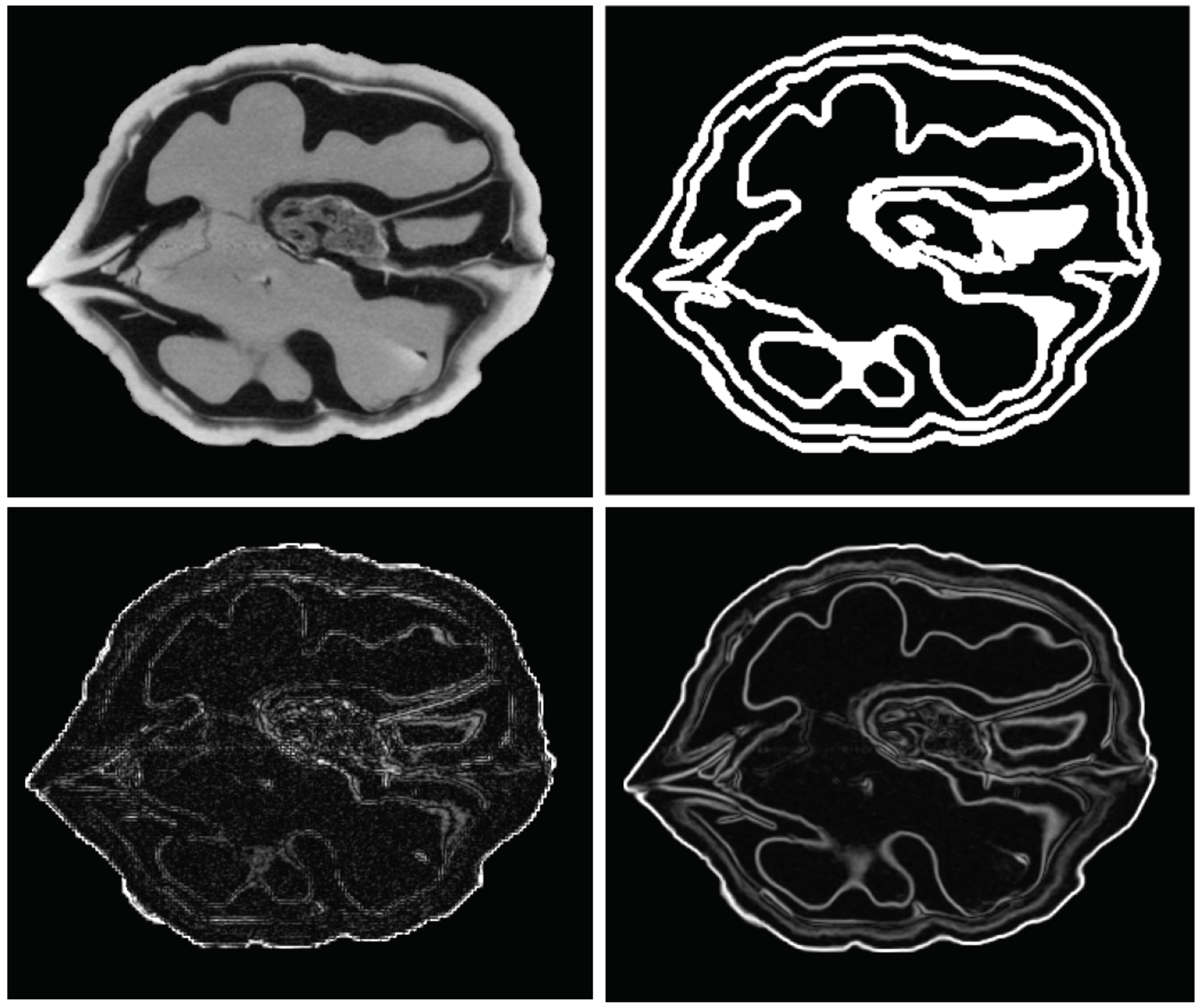
is larger. As an example, in Figure 4 (bottom left) a slice of the voxelwise interpolation error is shown.

We computed a VOI around the borders of the segmentation image as

$$\delta M=\underset{p=0}{\overset{n}{\vee }}\delta M_p$$

(35)

where ∨ means the logic OR operator, and each border $\delta M_p$ is computed as

$$\delta M_p=\mathrm{dilate}(M_p,3)\otimes \mathrm{erode}(M_p,3)$$

where ⊗ denotes the voxelwise logic xor operator, $\mathtt{dilate}(X,n)$ and $\mathtt{erode}(X,n)$ the binary erosion an dilation morphological operators repeated n times. Erosion and dilation operators are implemented in scikit-image Python package [38]. An example of $\delta M$ can be found in Figure 4 (top right).

We also estimate the 2-norm of the gradient of the high-resolution image I

$$\nabla I:={∥\left(\frac{\partial f}{\partial x},\frac{\partial f}{\partial y},\frac{\partial f}{\partial z}\right)∥}_2$$

(36)

where each partial derivative of the function f defined in (1) is estimated with Sobel operator (cf. [39]) in scikit-image. An example of $\nabla I$ is in Figure 4 (bottom right).

As a dissimilarity measure between images, we use the Dissimilarity Structural SIMilarity index (DSSIM), defined as

$$\mathrm{DSSIM}(A,B):=1-\mathrm{SSIM}(A,B)$$

where the Structural SIMilarity index (or SSIM, is a $[0,1]$-valued similarity measure which has been shown to be a stable metric for multivariate interpolation [8,40,41] and it is defined as

$$\mathrm{SSIM}(A,B)=\frac{(2\overline{A}\overline{B}+c_1)(2{\mathsf{\Sigma }}_{AB}+c_2)}{({\overline{A}}^2+{\overline{B}}^2+c_1)({\mathsf{\Sigma }}_A^2+{\mathsf{\Sigma }}_B^2+c_2)}$$

being $\overline{A}$ the mean, ${\mathsf{\Sigma }}_A$ the standard deviation, and $c_1,c_2$ two real default constants used for stability. For the tuning of the parameters $c_1,c_2$ refer e.g., to [40]. The SSIM of two identical images is 1, which means that the DSSIM is zero.

Using scikit-image we compute the global error $\mathrm{DSSIM}(I,F_{+})$, the error at the borders $\delta M$ as $\mathrm{DSSIM}(I\left[\delta M\right],F_{+}\left[\delta M\right])$ and the percent ratio between the two in order to assess how much of the error is located in the borders.

Moreover, we want to know how much of the image gradient is located at the borders and which part of the FOV volume is taken by the border in terms of number of voxels.

In fact although we expect an ideal segmentation to perfectly identify all of the different parts of the object in the FOV, in practice a segmentation can miss some signal discontinuity. We decided to take into account

$$\nabla I{\left[\delta M\right]}_{(\%)}:=\frac{{\parallel \nabla I\left[\delta M\right]\parallel }_1}{{\parallel \nabla I\parallel }_1}·100$$

as a measure of the ratio of the image gradient located in the VOIs border $\delta M$. Moreover, to ensure that $\delta M$ does not cover too much of the FOV—in such case a high gradient ratio would be unavoidable—we computed the Volume ratio

$$\mathrm{Vol}{\left(\delta M\right)}_{(\%)}:=\frac{\mathrm{Vol}\left(\delta M\right)}{\mathrm{meas}\left(\mathsf{\Omega }\right)}·100.$$

5. Experimental Results

The results of the VOI-wise analysis are shown in

Table 2. Relative errors in two-norm of the mean value per VOI, computed with Equation (33). Minimal error per software per image in red. Empty cells indicate the same as above.

Software	Sampling	Method	SL Phantom	Brain MRI	Walnut CT
ANTs	under	Nearest	0.11715	0.00251	0.00029
		MultiLabel	0.11714	0.00287	0.00098
	over	Linear	0.16559	0.02427	0.01965
		Gaussian	0.24197	0.05616	0.04605
		Lanczos	0.12989	0.01415	0.01425
		Splines	0.12790	0.00791	0.00751
FSL	under	Nearest	0.10845	0.00327	0.00383
	over	Trilinear	0.16528	0.02430	0.02025
		Splines	0.10403	0.00792	0.00759
Freesurfer	under	Nearest	0.11716	0.00252	0.00029
	over	Trilinear	0.16559	0.02427	0.01965
		Splines	0.12644	0.00792	0.00751

and

Table 3. Relative errors in ∞-norm of the mean value per VOI. Minimal error per software per image in red. Empty cells indicate the same as above.

Software	Sampling	Method	SL Phantom	Brain MRI	Walnut CT
ANTs	under	Nearest	0.12516	0.00425	0.00031
		MultiLabel	0.12515	0.00441	0.00106
	over	Linear	0.17679	0.03075	0.02246
		Gaussian	0.25852	0.06774	0.05099
		Lanczos	0.13884	0.01929	0.01661
		Splines	0.13646	0.01261	0.00940
FSL	under	Nearest	0.11173	0.00479	0.00526
	over	Trilinear	0.17663	0.03077	0.02322
		Splines	0.11108	0.01265	0.00953
Freesurfer	under	Nearest	0.12516	0.00425	0.00031
	over	Trilinear	0.17679	0.03075	0.02246
		Splines	0.13488	0.01262	0.00940

. In all the cases but one, undersampling the segmentation images leads to a smaller relative 2-norm error (and ∞-norm, respectively) on estimating the mean intensity in the VOIs.

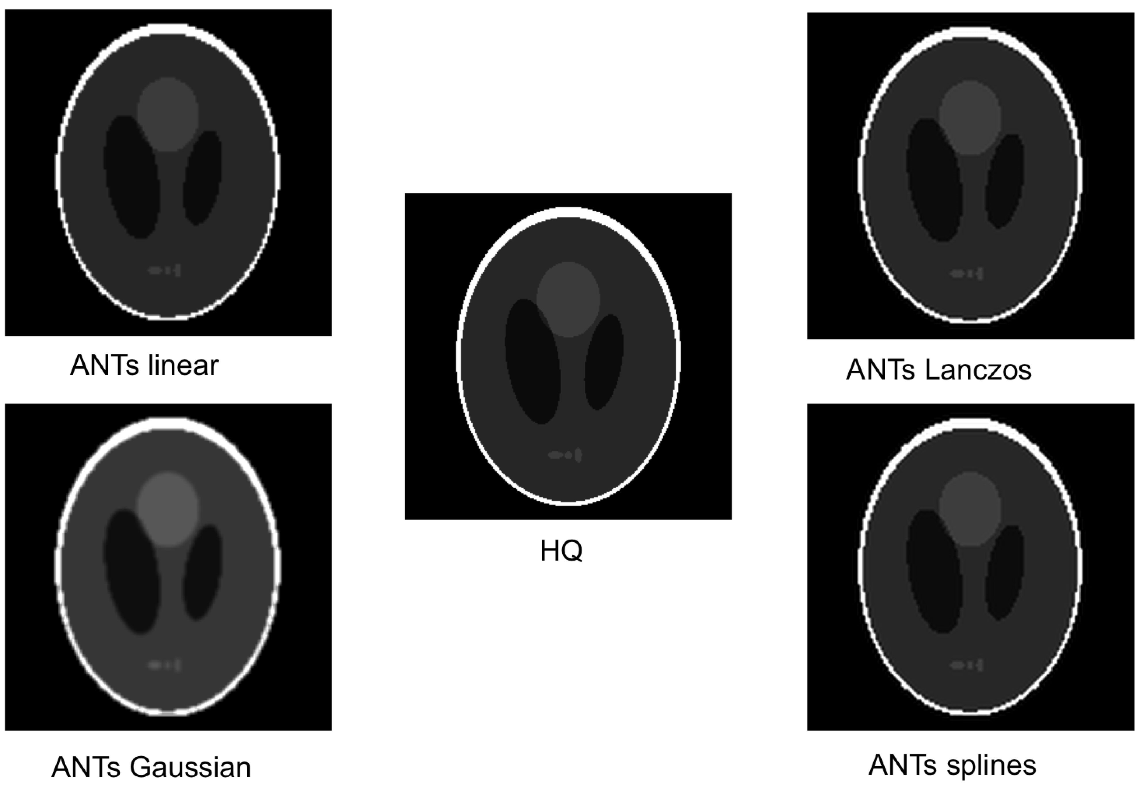
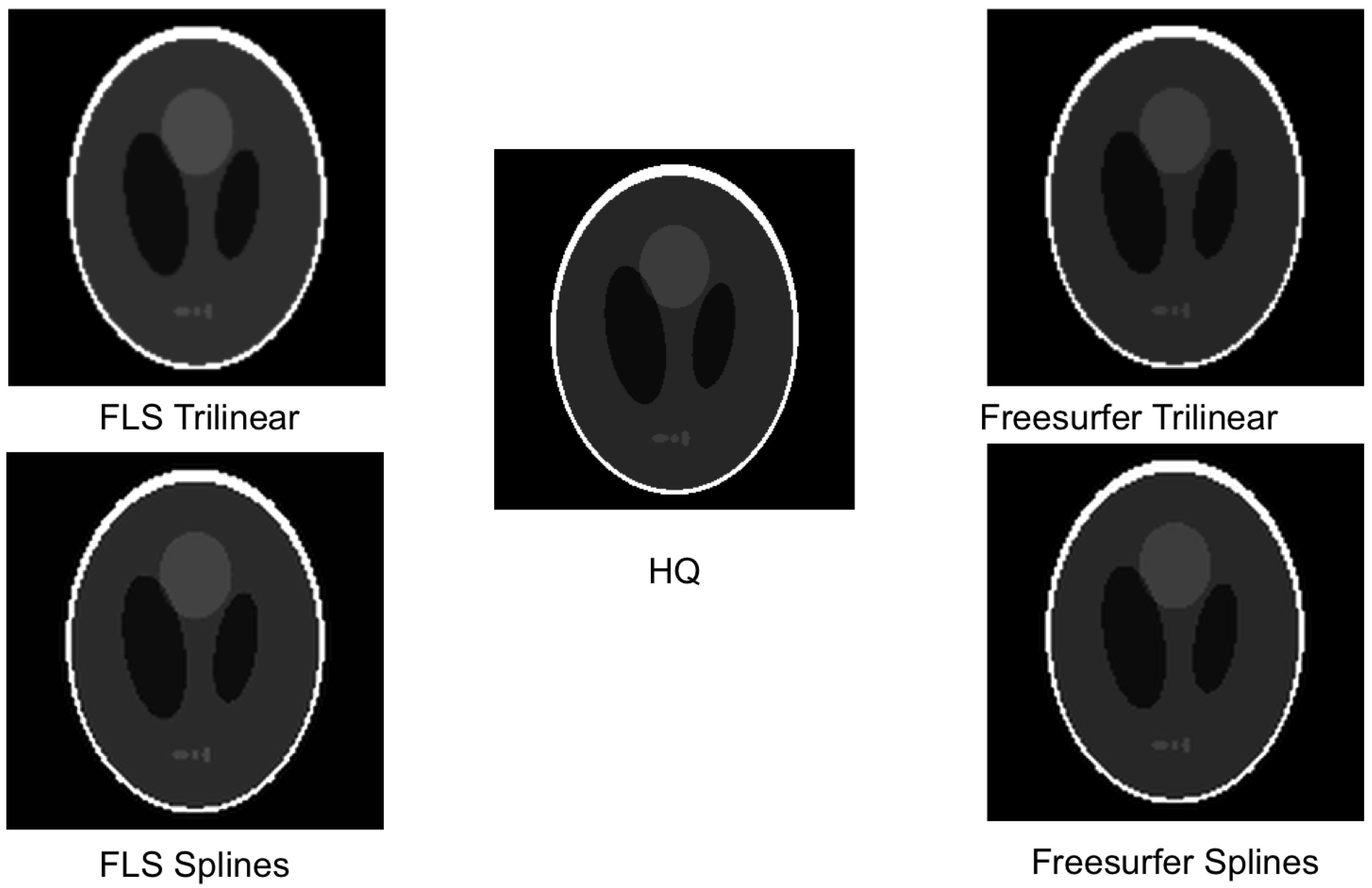
In Figure 5 and Figure 6 you can observe a comparison between a slice of the original, high quality Shepp–Logan phantom and the same slice of the oversampled images using all the methods used in this work. From these images it is possible to guess that for the most part the errors are located around the discontinuities.

In

Table 4. Interpolation oversampling errors in terms of $\mathrm{DSSIM}(I,F_{+})$ (the smaller the better), DSSIM at the segmentation border VOI $\mathrm{DSSIM}\left(\delta M\right)=\mathrm{DSSIM}(I\left[\delta M\right],F_{+}\left[\delta M\right])$ and its percentage. Per image, per method. Percentage of the image gradient at the borders $\delta M$ and percentage volume of $\delta M$ over the whole FOV. Empty cells indicate the same as above.

Image	Software	Method	DSSIM	DSSIM($\mathit{\delta }\mathit{M}$)	%	$\mathit{\nabla }\mathit{I}{\left[\mathit{\delta }\mathit{M}\right]}_{(\%)}$	$\mathbf{Vol}(\mathit{\delta }{\mathit{M})}_{(\%)}$
SL	ANTs	Linear	0.037153	0.031298	84.242829	100.000000	14.897966
		Gaussian	0.047003	0.038652	82.233787
		Lanczos	0.042190	0.035423	83.961040
		Splines	0.041255	0.034414	83.418321
	FSL	Trilinear	0.029491	0.023908	81.068121
		Splines	0.033593	0.027387	81.524186
	Freesurfer	Trilinear	0.037153	0.031298	84.242829
		Splines	0.038853	0.031272	80.488007
Brain	ANTs	Linear	0.062901	0.034254	54.457968	89.20926	18.886478
		Gaussian	0.111262	0.051932	46.675099
		Lanczos	0.080985	0.033880	41.835420
		Splines	0.102826	0.033518	32.596547
	FSL	Trilinear	0.062913	0.034261	54.457173
		Splines	0.102840	0.033526	32.599943
	Freesurfer	Trilinear	0.062901	0.034254	54.457961
		Splines	0.102826	0.033518	32.596537
Walnut	ANTs	Linear	0.044889	0.011284	25.137363	71.41374	14.234087
		Gaussian	0.091228	0.028299	31.020122
		Lanczos	0.079741	0.021932	27.503712
		Splines	0.114494	0.021974	19.191816
	FSL	Trilinear	0.046841	0.012816	27.360825
		Splines	0.114795	0.022474	19.577444
	Freesurfer	Trilinear	0.044889	0.011284	25.137374
		Splines	0.114494	0.021973	19.191790

the DDSIM and DSSIM at the borders are listed for each image, software and interpolation method. The ratio of the error located in the borders is 80 to 85% for the SL phantom, whose borders host the totality of the gradient, the phantom being a picewise-constant function. The brain image holds the 89% of the gradient and an error percentage of about 30–55%. The walnut image has the lowest gradient percentage (71%) and the lowest error percentage, spanning from 19 to 31%.

6. Discussion

The resampling paradox is confirmed by these data shown in Table 2, as the errors in estimating the mean value of the VOIs assessed by undersampling the segmentation image are smaller than any error produced by oversampling the functional images. The only exception is the splines interpolation in FSL, which seems to be produced by an error compensation in the computation of the mean values. This is confirmed by its DSSIM shown in Table 4, which is larger than the DSSIM given by the Trilinear interpolation in FSL.

These data also indicate that the interpolation error occurring in oversampling is a Gibbs effect, confirming the results proven in the theoretical section. As we can intuitively infer from Figure 4, the pointwise error is mostly located in voxels where the gradient is higher. This intuition is confirmed by inspecting Table 4 as the most of the error lies at the borders of the VOIs when the gradient at the border is higher and decreases in cases where the segmentation misses some high-gradient zones.

In the case of the walnut CT image, it can be observed in Figure 3 and Figure 4 that the provided segmentation misses some of the inner skin surrounding the seed and some gaps within the seed.

It is also noticeable that the error percentage in the borders has the tendency to be lower if the error is higher, possibly showing a propagation of the Gibbs effect around the borders.

7. Conclusions and Future Works

The Gibbs effect has been proven to appear in interpolation by convolution and is confirmed by experimental results to be the largest source of interpolation error in multimodal medical imaging.

The resampling paradox is confirmed experimentally. Undersampling is—as a matter of fact—the most chosen option in multimodal neuroimaging, despite the fact that the segmentation at high resolution results in a waste of effort and time.

In order to avoid this effect a new interpolation technique is needed allowing an oversampling of functional images which minimizes the Gibbs effect. This technique would permit extraction of more precise features of the functional images, and possibly enhance their statistical power following more trustful clinical assessments.

A promising approach is given by interpolation by convolution with the scale factor Point Spread Function (sfPSF) [42] which takes into account the different FWHM of the morphological and functional images. As an alternative, spectral filtering [6] could be a fast and efficient way of dealing with the Gibbs effect. Another interesting method we can consider is the Fake-Nodes interpolation introduced in [43], which has been shown to be an effective approach for univariate interpolation without resampling and multivariate approximation of data [44,45], reducing the Gibbs effect. Deep learning-based techniques for super-resolution can be also considered [46] when dealing with border-related oversampling errors.

References

1. Ehman, E.C.; Johnson, G.B.; Villanueva-Meyer, J.E.; Cha, S.; Leynes, A.P.; Larson, P.E.Z.; Hope, T.A. PET/MRI: Where might it replace PET/CT? J. Magn. Reson. Imaging 2017, 46, 1247–1262. [Google Scholar] [CrossRef] [Green Version]
2. Misri, R. Multimodality imaging, Molecular Imaging Techniques: New Frontiers. 2013, pp. 162–176. Available online: https://www.futuremedicine.com/doi/abs/10.4155/ebo.13.181 (accessed on 9 June 2021).
3. Zhang, X.Y.; Yang, Z.L.; Lu, G.M.; Yang, G.F.; Zhang, L.J. PET/MR Imaging: New Frontier in Alzheimer’s Disease and Other Dementias. Front. Mol. Neurosci. 2017, 10, 343. [Google Scholar] [CrossRef]
4. Cecchin, D.; Poggiali, D.; Riccardi, L.; Turco, P.; Bui, F.; De Marchi, S. Analytical and experimental FWHM of a gamma camera: Theoretical and practical issues. PeerJ 2015, 3, e722. [Google Scholar] [CrossRef] [Green Version]
5. Millman, K.J.; Brett, M. Analysis of Functional Magnetic Resonance Imaging in Python. Comput. Sci. Eng. 2007, 9, 52–55. [Google Scholar] [CrossRef]
6. De Marchi, S.; Erb, W.; Marchetti, F. Spectral filtering for the reduction of the gibbs phenomenon for polynomial approximation methods on lissajous curves with applications in MPI. Dolomites Res. Notes Approx. 2017, 10, 128–137. [Google Scholar] [CrossRef]
7. Tustison, N.J.; Avants, B.B.; Cook, P.A.; Kim, J.; Whyte, J.; Gee, J.C.; Stone, J.R. Logical circularity in voxel-based analysis: Normalization strategy may induce statistical bias. Hum. Brain Mapp. 2012, 35, 745–759. [Google Scholar] [CrossRef]
8. Dumitrescu, D.; Boiangiu, C.A. A Study of Image Upsampling and Downsampling Filters. Computers 2019, 8, 30. [Google Scholar] [CrossRef] [Green Version]
9. Delgado, J.; Moure, J.C.; Vives-Gilabert, Y.; Delfino, M.; Espinosa, A.; Gómez-Ansón, B. Improving the Execution Performance of FreeSurfer. Neuroinformatics 2014, 12, 413–421. [Google Scholar] [CrossRef]
10. Jerri, A. The Gibbs Phenomenon in Fourier Analysis, Splines, and Wavelet Approximations. Z. Angew. Math. Mech. 2005, 85, 224. [Google Scholar] [CrossRef]
11. Lehmann, T.; Gonner, C.; Spitzer, K. Survey: Interpolation methods in medical image processing. IEEE Trans. Med. Imaging 1999, 18, 1049–1075. [Google Scholar] [CrossRef] [Green Version]
12. Fischl, B.; Salat, D.H.; Busa, E.; Albert, M.; Dieterich, M.; Haselgrove, C.; van der Kouwe, A.; Killiany, R.; Kennedy, D.; Klaveness, S.; et al. Whole Brain Segmentation. Neuron 2002, 33, 341–355. [Google Scholar] [CrossRef] [Green Version]
13. Cecchin, D.; Barthel, H.; Poggiali, D.; Cagnin, A.; Tiepolt, S.; Zucchetta, P.; Turco, P.; Gallo, P.; Frigo, A.C.; Sabri, O.; et al. A new integrated dual time-point amyloid PET/MRI data analysis method. Eur. J. Nucl. Med. Mol. Imaging 2017, 44, 2060–2072. [Google Scholar] [CrossRef]
14. Fornberg, B.; Flyer, N. The Gibbs phenomenon for radial basis functions. In The Gibbs Phenomenon in Various Representations and Applications; Sampling Publishing: Potsdam, NY, USA, 2006. [Google Scholar]
15. Chhoa, J.F. An Adaptive Approach to Gibbs’ Phenomenon. Master’s Thesis, The University of Southern Mississippi, Hattiesburg, MS, USA, 2020. [Google Scholar]
16. Hamann, B. Modeling contours of trivariate data. ESAIM M2AN 1992, 26, 51–75. [Google Scholar] [CrossRef] [Green Version]
17. Haralick, R.M.; Sternberg, S.R.; Zhuang, X. Image Analysis Using Mathematical Morphology. IEEE Trans. Pattern Anal. Mach. Intell. 1987, 4, 532–550. [Google Scholar] [CrossRef] [PubMed]
18. Pham, D.L.; Xu, C.; Prince, J.L. Current Methods in Medical Image Segmentation. Annu. Rev. Biomed. Eng. 2000, 2, 315–337. [Google Scholar] [CrossRef] [PubMed]
19. Hu, M.K. Visual pattern recognition by moment invariants. IEEE Trans. Inform. Theory 1962, 8, 179–187. [Google Scholar] [CrossRef] [Green Version]
20. Klęsk, P.; Kapruziak, M.; Olech, B. Statistical moments calculated via integral images in application to landmine detection from Ground Penetrating Radar 3D scans. Pattern Anal. Applic 2017, 21, 671–684. [Google Scholar] [CrossRef] [Green Version]
21. Burger, W.; Burge, M.J. Principles of Digital Image Processing: Core Algorithms; Springer: Berlin/Heidelberg, Germany, 2009; pp. 210–233. [Google Scholar]
22. Moraes, T.; Amorim, P.; Da Silva, J.V.; Pedrini, H. Medical image interpolation based on 3D Lanczos filtering. Comput. Methods Biomech. Biomed. Eng. Imaging Vis. 2019, 8, 294–300. [Google Scholar] [CrossRef]
23. Getreuer, P. Linear Methods for Image Interpolation. Image Process. Line 2011, 1, 238–259. [Google Scholar] [CrossRef] [Green Version]
24. Wendland, H. Fast Evaluation of Radial Basis Functions: Methods Based on Partition of Unity. In Approximation Theory X: Wavelets, Splines, and Applications; Vanderbilt University Press: Nashville, TN, USA, 2002; pp. 473–483. [Google Scholar]
25. Jung, J.H. A note on the Gibbs phenomenon with multiquadric radial basis functions. Appl. Numer. Math. 2007, 57, 213–229. [Google Scholar] [CrossRef]
26. Shepp, L.; Logan, B. The Fourier reconstruction of a head section. IEEE Trans. Nucl. Sci. 1974, 21, 21–43. [Google Scholar] [CrossRef]
27. Brett, M.; Markiewicz, C.J.; Hanke, M.; Côté, M.A.; Cipollini, B.; McCarthy, P.; Jarecka, D.; Cheng, C.P.; Halchenko, Y.O.; Cottaar, M.; et al. nipy/nibabel: 3.2.1. Zenodo 2020. [Google Scholar] [CrossRef]
28. Cardoso, M.J.; Modat, M.; Wolz, R.; Melbourne, A.; Cash, D.; Rueckert, D.; Ourselin, S. Geodesic Information Flows: Spatially-variant Graphs and Their Application to Segmentation and Fusion. IEEE Trans. Med. Imaging 2015, 34, 1976–1988. [Google Scholar] [CrossRef] [Green Version]
29. Prassni, J.S.; Ropinski, T.; Hinrichs, K. Uncertainty-Aware Guided Volume Segmentation. IEEE Trans. Vis. Comput. Graph. 2010, 16, 1358–1365. [Google Scholar] [CrossRef]
30. Müller-Gärtner, H.W.; Links, J.M.; Prince, J.L.; Bryan, R.N.; McVeigh, E.; Leal, J.P.; Davatzikos, C.; Frost, J.J. Measurement of Radiotracer Concentration in Brain Gray Matter Using Positron Emission Tomography: Mri-based Correction for Partial Volume Effects. J. Cereb. Blood Flow Metab. 1992, 12, 571–583. [Google Scholar] [CrossRef] [Green Version]
31. Avants, B.; Epstein, C.; Grossman, M.; Gee, J. Symmetric diffeomorphic image registration with cross-correlation: Evaluating automated labeling of elderly and neurodegenerative brain. Med. Image Anal. 2008, 12, 26–41. [Google Scholar] [CrossRef] [Green Version]
32. Avants, B.B.; Tustison, N.J.; Song, G.; Cook, P.A.; Klein, A.; Gee, J.C. A reproducible evaluation of ANTs similarity metric performance in brain image registration. Neuroimage 2011, 54, 2033–2044. [Google Scholar] [CrossRef] [Green Version]
33. Jenkinson, M.; Beckmann, C.F.; Behrens, T.E.; Woolrich, M.W.; Smith, S.M. Fsl. Neuroimage 2012, 62, 782–790. [Google Scholar] [CrossRef] [Green Version]
34. Reuter, M.; Rosas, H.D.; Fischl, B. Highly accurate inverse consistent registration: A robust approach. Neuroimage 2010, 53, 1181–1196. [Google Scholar] [CrossRef] [Green Version]
35. Smith, S.M.; Jenkinson, M.; Woolrich, M.W.; Beckmann, C.F.; Behrens, T.E.; Johansen-Berg, H.; Bannister, P.R.; De Luca, M.; Drobnjak, I.; Flitney, D.E.; et al. Advances in functional and structural MR image analysis and implementation as FSL. Neuroimage 2004, 23. [Google Scholar] [CrossRef] [Green Version]
36. Zou, K.H.; Warfield, S.K.; Bharatha, A.; Tempany, C.M.; Kaus, M.R.; Haker, S.J.; Wells, W.M.; Jolesz, F.A.; Kikinis, R. Statistical validation of image segmentation quality based on a spatial overlap index1. Acad. Radiol. 2004, 11, 178–189. [Google Scholar] [CrossRef] [Green Version]
37. Mccormick, M.; Liu, X.; Jomier, J.; Marion, C.; Ibanez, L. ITK: Enabling reproducible research and open science. Front. Neuroinform. 2014, 8. [Google Scholar] [CrossRef] [PubMed]
38. van der Walt, S.; Schönberger, J.L.; Nunez-Iglesias, J.; Boulogne, F.; Warner, J.D.; Yager, N.; Gouillart, E.; Yu, T. Scikit-image: Image processing in Python. PeerJ 2014, 2, e453. [Google Scholar] [CrossRef] [PubMed]
39. Kittler, J. On the accuracy of the Sobel edge detector. Image Vision Comput. 1983, 1, 37–42. [Google Scholar] [CrossRef]
40. Wang, Z.; Bovik, A.C.; Sheikh, H.R.; Simoncelli, E.P. Image quality assessment: From error visibility to structural similarity. IEEE Trans. Image Process. 2004, 13, 600–612. [Google Scholar] [CrossRef] [PubMed] [Green Version]
41. Marchetti, F. In Convergence rate in terms of the continuous SSIM (cSSIM) index in RBF interpolation. Dolomites Res. Notes Approx. 2021, 14. Available online: https://drna.padovauniversitypress.it/2021/1/31 (accessed on 9 June 2021).
42. Cardoso, M.J.; Modat, M.; Vercauteren, T.; Ourselin, S. Scale factor point spread function matching: Beyond aliasing in image resampling. In International Conference on Medical Image Computing and Computer-Assisted Intervention; Lecture Notes in Computer Science (Including Subseries Lecture Notes in Artificial Intelligence and Lecture Notes in Bioinformatics); Springer: Berlin/Heidelberg, Germany, 2015; Volume 9350, pp. 675–683. [Google Scholar] [CrossRef]
43. De Marchi, S.; Marchetti, F.; Perracchione, E.; Poggiali, D. Polynomial interpolation via mapped bases without resampling. J. Comput. Appl. Math. 2020, 364, 112347. [Google Scholar] [CrossRef]
44. De Marchi, S.; Erb, W.; Francomano, E.; Marchetti, F.; Perracchione, E.; Poggiali, D. Fake Nodes approximation for Magnetic Particle Imaging. In Proceedings of the 2020 IEEE 20th Mediterranean Electrotechnical Conference (MELECON), Palermo, Italy, 16–18 June 2020; pp. 434–438. [Google Scholar] [CrossRef]
45. De Marchi, S.; Marchetti, F.; Perracchione, E.; Poggiali, D. Multivariate approximation at fake nodes. Appl. Math. Comput. 2021, 391, 125628. [Google Scholar] [CrossRef]
46. Li, Y.; Iwamoto, Y.; Lin, L.; Xu, R.; Tong, R.; Chen, Y.W. VolumeNet: A Lightweight Parallel Network for Super-Resolution of MR and CT Volumetric Data. IEEE Trans. Image Process. 2021, 30, 4840–4854. [Google Scholar] [CrossRef] [PubMed]
Figure 1. From left to right: Truncated Fourier series, polynomial interpolation (on Chebyshev–Lobatto nodes) and cubic splines interpolation (on equispaced nodes) of the Heaviside step function.
Mathematics 09 01348 g001
Figure 2. Ringing effect in a Shepp–Logan phantom. The effect has been magnified for visualization purposes.
Mathematics 09 01348 g002
Figure 3. From left to right: a slice of the the SL phantom, Brain MRI and walnut CT. In the second row are the corresponding segmentation images, with a different color used for each different VOI.
Mathematics 09 01348 g003
Figure 4. Upper left: a slice of the walnut CT I. Upper right: the borders δ M computed as in Equation (35) at the same slice. Bottom left: the pointwise absolute error E (as in Equation (34)) in ANTs linear interpolation. Bottom right: I , the norm of the gradient of the original image computed with Equation (36).
Mathematics 09 01348 g004
Figure 5. A slice of the Shepp–Logan phantom in High Resolution (center), and oversampled in ANTs with four different basis functions (all around).
Mathematics 09 01348 g005
Figure 6. A slice of the Shepp–Logan phantom in High Resolution (center), and oversampled in FLS (left) and Freesurfer (right) using the Trilinear (top) and Splines (bottom) basis function, respectively.
Mathematics 09 01348 g006