1. Introduction
Wildfires are becoming a major concern for societies around the globe, and research shows that changes in climate are going to alter the amount and size of wildfires in specific regions [
1,
2,
3,
4]. The effects are diverse depending on many factors, like weather conditions, vegetation affected, land cover, land management before and after the incident, the geographical region affected, or human vegetation management and risk mitigation. Wildfires occur by a combination of conditions created either by human intervention (e.g., power lines failures [
5]) or by unpredictable events (such as lightnings [
6,
7], and thus are much harder to anticipate). As natural environments become more vulnerable to this kind of events, cities and inhabitable places need to be made more resilient, as they are likely to become more frequent due to changes in climate [
3]. The result of these events increasing in size and frequency is hard to capture, as the amount of ecosystems and populations affected by these is very large.
Remote sensing can be defined as “the science of observation from a distance" [
8], including many types of sensors. In this study, we are particularly interested in satellite images. These have become an invaluable and increasingly popular research field of study in the last few decades. Observation of the Earth from a distance has enormous potential. It allows monitoring and capturing changes in environments around the world, enabling their detection, quantification and possible prevention, which makes the modification of human environments more sustainable. Historically, natural disasters have played an important role in shaping societies, as these pose a significant threat in some regions on Earth. In order to create resilient and sustainable communities, remote sensing tools can help adapt to these events [
9,
10,
11], and help build environmental policies to protect Earth as we know it [
12]. In this work, we are focusing on how wildfires affect vegetation and how environments recover from these catastrophic events. Remote sensing plays a critical role for assessing the impact of wildfires and learning to coexist with these events [
13]. We use Functional Data Analysis (FDA, [
14]) to analyze wildfire dynamics from remote sensing data. This work is part of the growing literature on FDA for remote sensing data (see, e.g., [
15,
16,
17] among others).
Information from remote sensing provides a very important temporal component that allows studying and quantifying the dynamical evolution of the effects of wildfires and recoveries over time. Specifically, ref. [
18] uses various sources of remote sensing data, combined with synthetic controls for assessing the vegetation impacts of wildfires over time. In this study, we analyze these recoveries processes as functional data. Each observation measures over several years how the vegetation evolves in a specific region that suffered from a large wildfire, and it represents the decrease or loss of vegetation (that will be defined in the next sections) from each wildfire, as a function of time
t, starting at the time of the wildfire up until 7 years after the wildfire, showing the recovery of vegetation from these events.
Hence, the aim of this study is to explain the effects of wildfires on vegetation from remote sensing (satellite) images through FDA, as an alternative approach to classical regression methodologies used to study the effects of wildfires. Classical models usually summarize the whole recovery by comparing few periods of time, pre- and post-wildfire [
19]. We take advantage of remote sensing technologies and modern statistical tools to answer questions like the following:
- (i)
What are the effects of wildfires on different kinds of environments?
- (ii)
Do the wildfire effects evolution depend on the vegetation of the burned area?
- (iii)
Can we explain recoveries of vegetation from wildfires using pre-wildfire observable covariates?
This study is focused on medium to large wildfires (≥1000 acres, or 404 hectares) in California throughout a time-span of two decades (1996–2016). We explain the recoveries of vegetation from wildfires using pre-wildfire vegetation conditions and other characteristics of the affected lands using FDA. One of the main advantages from this methodology is that we can use the whole recovery process as a function of time.
Previous studies use differences between pre- and post-wildfire occurrence, showing relative difference between values over fixed time periods, or comparisons of few wildfires (e.g., a dozen wildfires [
20], 3 or 5 years after the event [
21,
22]). This results in raster maps of differences between few time periods, gaining insights on the exact locations where vegetation has decreased. However, this approach lacks the temporal nature of the problem, as vegetation changes over time in a continuous manner.
In order to estimate the dynamical causal effects of wildfires, causal inference through synthetic controls was used in [
18]. This methodology comes from the combination of Econometrics and Political Science, and it consists on the estimation of a hypothetical scenario (a counterfactual) with the absence of a wildfire (the intervention). Thus, in the present case, health vegetation indices were estimated in places where there were wildfires, as if the wildfires had not happened, using a Generalized Synthetic Control (GSC) methodology [
23]. Then, the wildfire effect was estimated as the difference between the observed indices and the estimated counterfactuals. Usually the size of the wildfire effect decreases over time so we also refer as wildfire recovery to the wildfire effect as a function of time.
We use seasonality adjustment techniques to extract the trend of the wildfire effects estimated in the previous study. Then proceed to regress these effects, measured over time, using Functional Regression Models. More precisely, we regress functional responses on scalar covariates. This results in estimated coefficients changing over time that provide insights into different questions, as the ones stated above.
This paper is structured as follows. First, we introduce the used data and their pre-processing, as well as the algorithms used to obtain the outcomes to be predicted. Next, we explain the methodology that will be used in this study. Then, we show the attained results and summarize the key findings derived from this study. Last, we discuss the potential impact of these results and conclude with final notes.
3. Methods
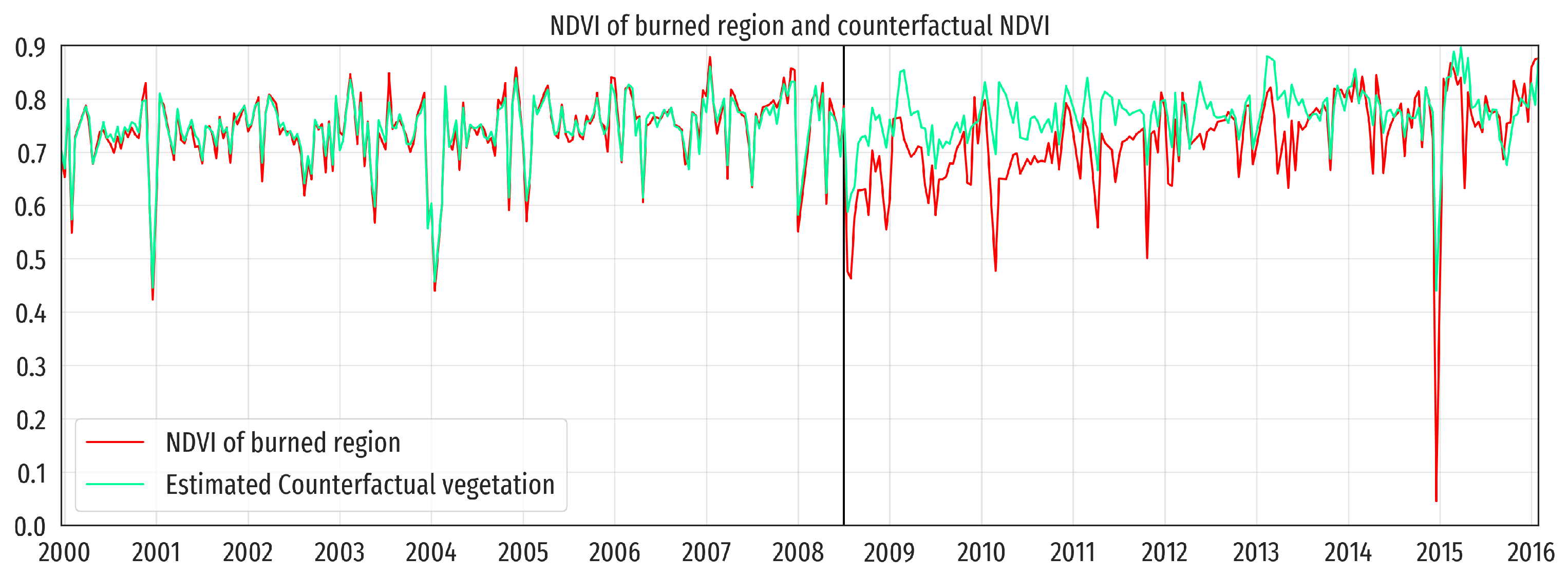
NDVI time series usually present seasonality, as vegetation changes throughout the seasons of the year. This is especially evident for some types of vegetation, such as grasslands or shrublands. Therefore, we expect post-wildfire NDVI time series of both, the observed and the estimated counterfactual vegetation indices, to present seasonal components. These seasonal components will have different amplitudes, since the burned region will present distinct seasonal patterns during the recovery. Therefore, the difference between the burned region NDVI and the counterfactual NDVI will presumably present a changing seasonal pattern.
Note that, when aligning all the timings of the wildfires, the seasonal pattern of each particular wildfire will present a different phase, as the timings throughout the year of wildfires are different: some wildfires occur on summer periods as opposed to the ones that occur during early spring. Hence, before aligning the recoveries for all wildfires, to conform a unique functional dataset with no mismatches in the phases of seasonality we need to extract the seasonal pattern of each wildfire separately.
In addition, several aspects of the remote sensed data can produce measurement error. Even though pixels that captured clouds were not included at the timing of aggregating multispectral data to measure vegetation, other types of noise could have potentially leaked in the data. To reduce the amount of noise and extract recoveries of vegetation from wildfires, it is suitable for this analysis to smooth the data.
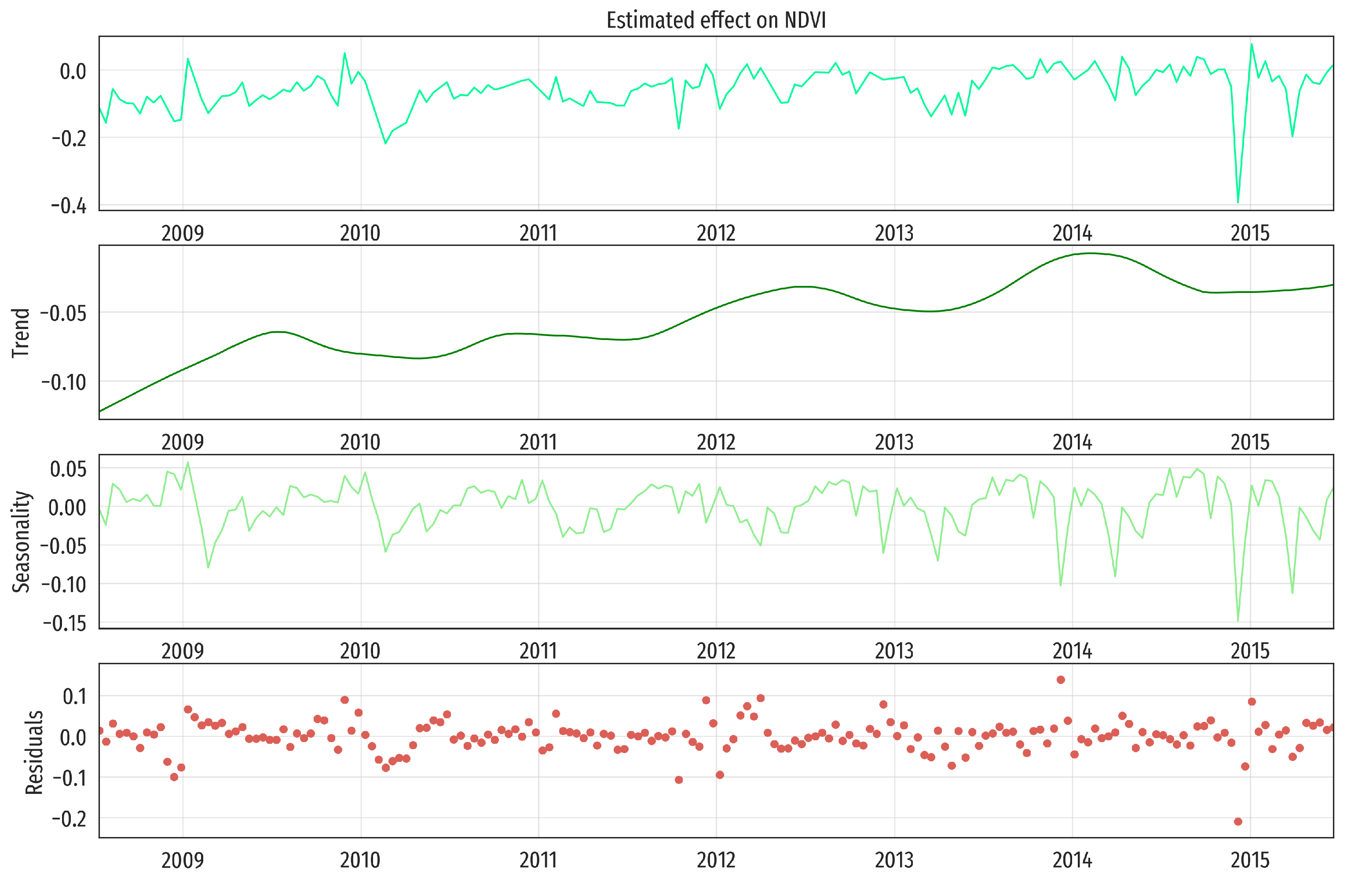
Therefore, for each time series, we perform a LOcally Estimated Scatterplot Smoothing (LOESS) decomposition, that will simultaneously remove the individual seasonality from the time series, as well as remove noise from the remotely sensed data.
3.1. Trend Extraction with LOESS and Functional Representation of Data
Once the effects for each wildfire are obtained, we decompose the time series into its structural components. Trend extraction of univariate data is a wide field of study [
32], where the classical decomposition model [
33] is a time series decomposed in additive terms, separating trend, seasonal component and residuals. Assuming the time series can be expressed as the addition of separate terms, for a wildfire starting at calendar time
(in years) we have
where
is the outcome observed
y at time
for
,
is the trend component at time
t,
is the seasonal component, which is approximately periodic with cycles of length one year (26 instants of time) in our case, and
is the residual component of the time series.
One method commonly used in many fields for time series decomposition is the seasonal-trend decomposition procedure using LOESS [
34], that is based on local polynomial fitting. This procedure presents several advantages, such as the flexibility on the trend and seasonal components extraction or the ability to decompose series with missing values.
We use the LOESS implementation from the Python [
35] library
statsmodels [
36] to extract the trend from the wildfire effects time series, removing the seasonal and the residual components at once.
Figure 4 shows an example of the time series decomposition in the MEU LIGHTNING COMPLEX (MIDDLE) example.
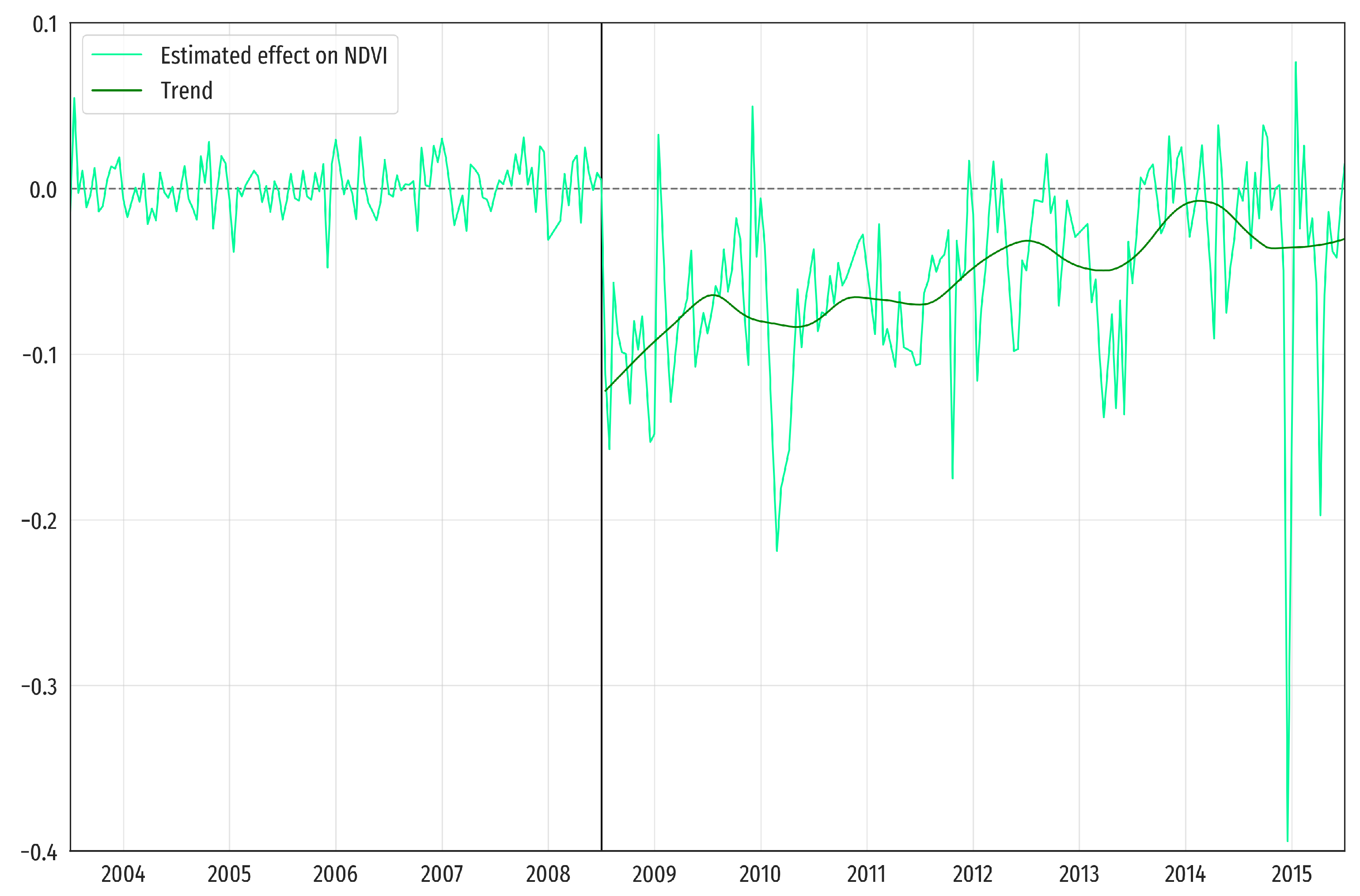
Figure 3 also shows (in dark green) the extracted trend over the estimated effect (in light green).
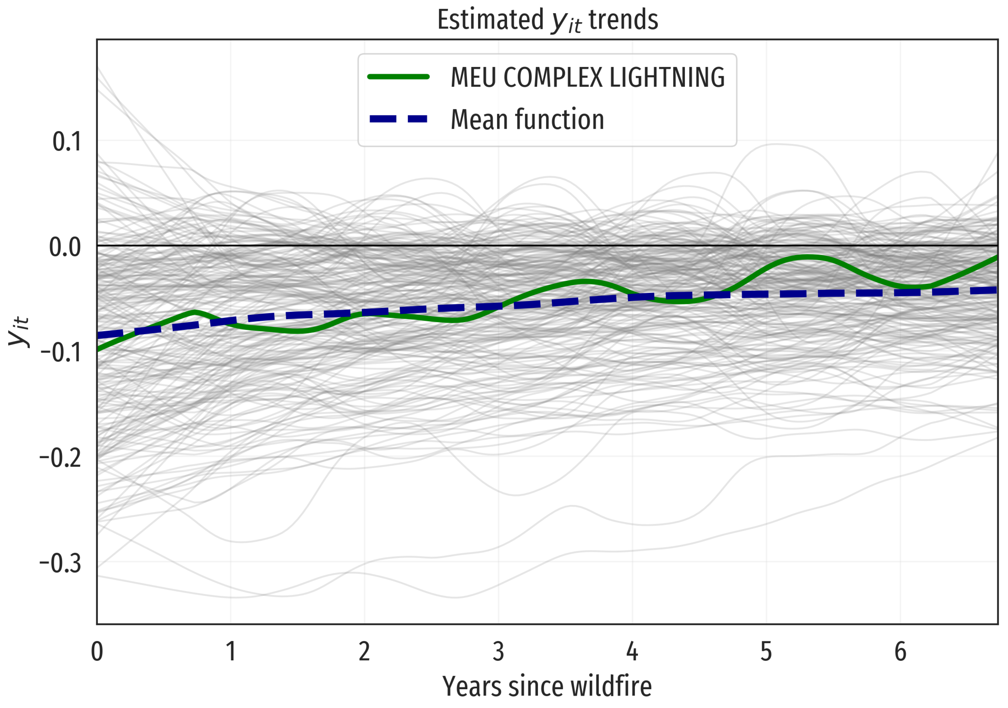
Finally, we align all the extracted trends at
and represent them as functional data. Each of the 243 wildfires is now represented by a function over 7 years of recovery. Each year of data contains 26 discrete values for each observation.
Figure 5 shows the functional dataset of NDVI trend recoveries, jointly with their mean function. The MEU LIGHTNING COMPLEX (MIDDLE) wildfire example is also highlighted in the figure. Raw data representation has been used for these functional data, that is, every function is represented as a column vectors with
j-th element equal to the value of the function at time
, for
.
3.2. Functional Principal Components Analysis
Functional Principal Component Analysis (FPCA; see, for instance, [
14] or [
37]) is a dimensionality reduction technique for functional data that generalizes the well known Principal Component Analysis extensively used for multivariate data.
Consider a functional dataset
with elements in
, the set of square integrable functions defined on
equiped with the inner product
. It is assumed that these functional data are independent realizations of a functional random variable
Y. The main objective of the FPCA is to determine the main modes of variation of the observed functions around the mean function. Formally, FPCA can be stated as follows. Let
be the mean function of the observed functional data. FPCA looks for functions
in
(principal functions) and real numbers (scores)
,
,
, such that
is minimum. Moreover, the functions
are required to be orthonormal (
). In other words, we are looking for a representation of functional data in the
q-dimensional space spanned by the functions
:
For
, the empirical covariance function is defined as
It can be proven that the principal functions are the eigen-functions corresponding to the largest
q eigenvalues of the sampling covariance operator, that is,
with
.
Moreover the score of the i-th functional data on the j-th principal function is .
The numerical computation of the functional principal components can be performed in different ways. We follow the proposal of [
14] (Chapters 8 and 9), based on cubic B-spline bases expansions of both, the observed functional data and the eigenfunctions of the sampling covariance operator.
Let
a cubic B-spline basis on the interval
. We consider the expansion of the centered functional data in this basis:
that we write in vector notation as
, where
and
. Then
where
.
For a generic
, let
be the expansion of
f in the cubic B-spline basis. Then
, with
. It can be proven that the first eigenfunction of the sampling covariance operator is also the solution of
. However,
Then
is (almost) equivalent to
and the problem reduces to the diagonalization of
. Let
be the eigenvector associated with its largest eigenvalue. Then we take
and the first eigenfunction we are looking for is
.
For obtaining successive eigenfunctions, it must be taken into account that two functions and are orthogonal if and only if . Therefore finding the eigenfunctions of the sampling covariance operator reduces to looking for the eigenvalues of the matrix .
In this approach to FPCA the smoothness of the principal functions
is inherited from the smoothness of the observed functional data
via the empirical covariance function
. Nevertheless it is possible to force smoothness in the eigenvalues explicitly performing a regularized version of FPCA (see [
14] (Chapter 9)). To do so, the problem to be solved is
for som
, where
is the second derivative of
f and the maximization is done in the space of functions
for which
is also in
. It is easy to see that this problem with
is equivalent to the previously considered FPCA problem, namely
. In [
14], is proved that the regularized FPCA can numerically solved by the diagonalization of the matrix
where
, and
is the
matrix with generic
element
.
3.3. Functional Regression Models
Analogous to classical regression models, Functional Regression Models (FRM) regress outcomes based on covariates when using functions as either the outcomes or regressors. Hence, FRM take advantage of the nature of time changing variables, either parametrically or non-parametrically. To do so, it can use the functional representation of both regressors and/or outcomes.
3.3.1. Function-on-Scalar Regression
In this research we use the function-on-scalar regression methodology (see, e.g., [
14,
38,
39]) as it allows us to understand the relation between the observed outcome over time, with respect to the fixed covariates observed. Let
be a pair of random variables, where
Y is functional and
is a random vector of dimension
k. The linear function-on-scalar regression model for
Y given
is stated as
where
is the functional response over time
for the observation
i,
is the value of variable
in the observation
i,
is the functional intercept (it is equal to the mean function
when the
k covariates are centered),
is the functional coefficient for the
j-th covariate
for
, and
is the functional error for the
i-th observation, a zero mean continuous stochastic process, assumed to be indpendent for different observations. The problem of variable selection in the linear function-on-scalar regression model was addressed in [
40].
However, different kinds of covariates can be considered, as not all of them have a changing effect over time, or might have different effects. In order to allow the function-on-scalar regression model to admit richer covariate terms, ref. [
41] introduced the functional additive mixed model (where functional covariates are also allowed). As an example, the following equation shows a function-on-scalar additive regression model with terms of different types:
where
is the functional intercept,
is constant over time,
is a smooth function of the covariate,
is the same kind of covariate-coefficient relation from Equation (
1),
is a smooth function depending on
t and
, and finally
is the
i-th error function. Variable selection is less developed for the function-on-scalar additive model than for the linear function-on-scalar model.
In the estimation of model (
2), the response functions
have been represented as raw data, that is, as a column vector
with
as the
j-th entry, where
. Coefficient functions
,
, are represented by their expansion in a cubic B-spline basis:
. The smooth functions of the covariates, as
, are represented also by expansions in a cubic B-spline basis over the range of the corresponding explanatory variable. For instance,
. Finally, smooth functions depending on
t and an explanatory variable, as
, are represented by their expansions in a tensor product basis. For instance,
, where
, and
is the vector formed by concatenation of the columns of matrix
M. Using these representations, for the
i-th observation, model (
2) can be written as
where
denotes the
N-vector of ones,
is the
matrix with element
equal to
, and
denotes the Kronecker product of matrices
and
, and
is the raw data representation of the functional noise
. Following [
41], model (
3) can be expressed as
where
and
can be partitioned into 5 blocks, each corresponding to a term in (
3). Let
be the partition corresponding to the parameters.
Assuming white noise, that is
, the penalized likelihood criterium to be minimized for estimating the model is
where matrices
in the the penalty terms are known positive semi-definite matrices, related with the integral of products of the second derivatives of the elements in the B-splines basis used in the smoothing terms. The smoothing parameters
control the trade-off between goodness of fit to the training data, and smoothness of the non-parametrically estimated functions of
t and/or
. The proposal in [
41] is to adopt a linear mixed effects model approach to the estimation process, in which the model parameters
and the smoothing parameters
are estimated simultaneously by restricted maximum likelihood (REML), as it is done in the R library
mgcv ([
42]) upon which [
41] base the function
pffr in their library
refund, for estimating models as (
2).
4. Results
In this section, we present the main results from this study, showing how the characteristics of the vegetation and land cover previous to the wildfire, as well as the prior weather conditions to the wildfire, affect the vegetation recovery patterns.
We start summarizing the functional dataset containing the 243 wildfire recoveries. Their mean function is represented in
Figure 5, jointly with the complete dataset. The mean wildfire effect on NDVI is always negative for the 7 year period after the wildfire, and the absolute value of this negative effect is monotonically decreasing over time, going from
at time 0 to
seven years later, in terms of lost NDVI points, with a global average of
. In average, the burned areas are progressively recovering
NDVI points after wildfires (approximately 10% of the range of the functional data set values, see
Figure 5). It is also noticeable that, on average, it takes more than 7 years for a complete recovery of the NDVI: the value of the mean function after 7 years is still negative. The library
fda.usc [
43] in R [
44] has been used for the descriptive analysis, including the choice of the MEU LIGHTNING COMPLEX (MIDDLE) as an illustrative wildfire example, as it has the modal median recovery function in 2008 (the modal year).
Next, FPCA has been applied to find the main modes of variation of the studied functional data around the average.
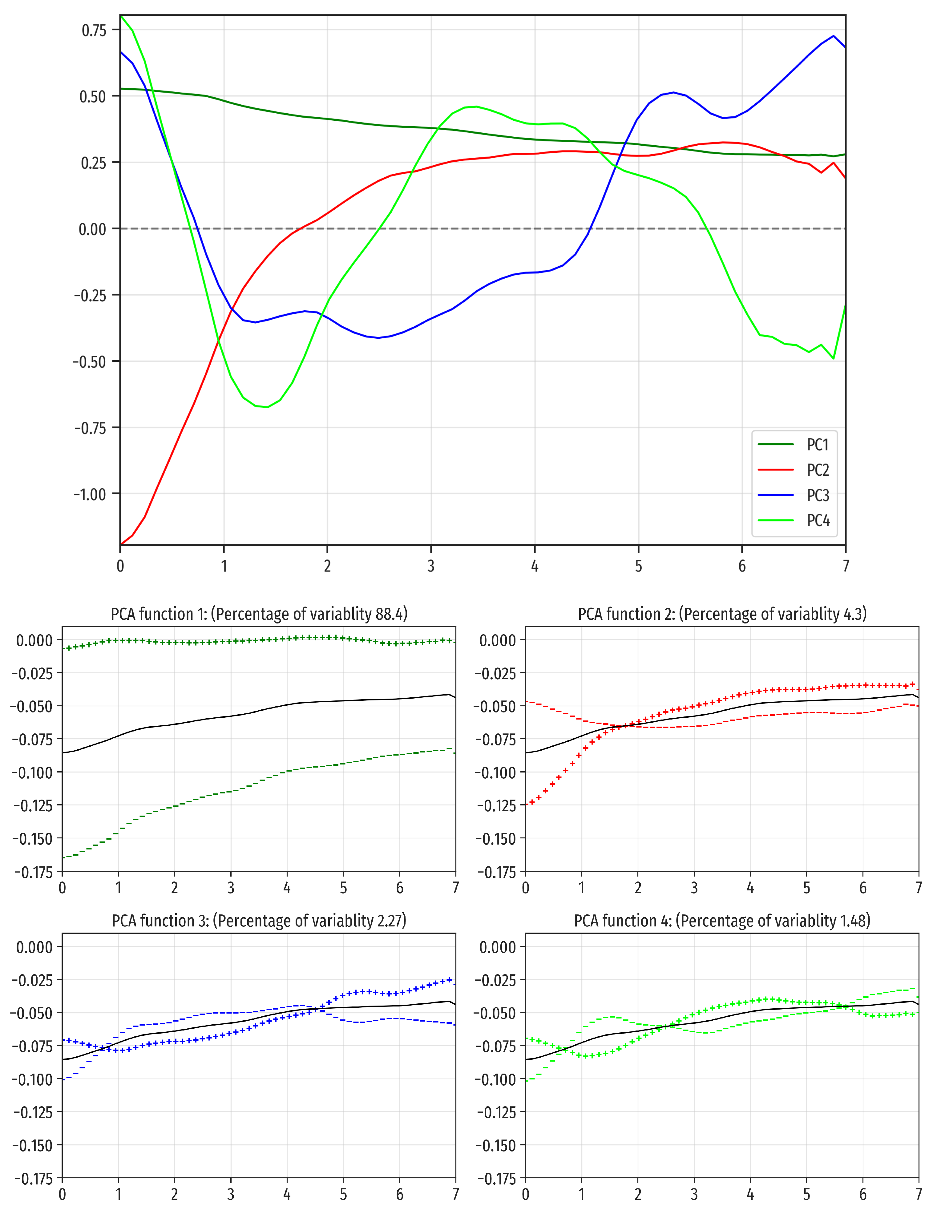
Figure 6 shows the mean, and the mean plus/minus a constant times the first four principal functions, that have been computed using the function
pca.fd from package
fda [
45] in R, as described in
Section 3.2. In particular, the number of functions in the B-spline basis has been
and the penalty parameter
. These choices have been determined when using the function
fdata2fd from library
fda.usc with default parameters to transform the raw functional data into a
fd class object of library
fda.
The first principal function explains almost 90% of the variability, showing a direction of severity in the NDVI drop: wildfires with positive scores in this principal function experiment smaller drops in NDVI than those having negative scores. The second principal function (4.3% of the total variability) can be interpreted as a direction separating wildfires with faster recoveries (those with more positive scores) from those with slower regeneration capacity (wildfires with more negative scores). The following two functional components only explain less than 4% of the total variance, with no clear recovery patterns, so they should be interpreted with caution.
The main goal of this study is to quantify the influence that different pre-wildfire conditions (geographical region, climatological conditions, or vegetation types) of the burned areas have on wildfire effects over the subsequent years post-wildfire. In order to achieve this goal, function-on-scalar additive models (of the type from Equation (
2)) are fitted using the function
pffr from the library
refund [
46] in R. The list of potential covariates to be included in this model is given in
Table 1. The number of functions in the B-Spline basis in all of these fitted models are the default values suggested by the
pffr function: 20 for the functional intercept
, 5 for smoothing terms depending on
t (for instance,
and
in model (
2)), and 10 for smoothing terms depending on other covariates (for instance,
and
in model (
2)). Notice that terms as
need two bases, one in the dimension of
t and the other in the dimension of the explanatory variable
.
As far as we know, the variable selection problem for the function-on-scalar additive model is still an open issue, as we mentioned in
Section 3.3.1. In fact, library
refund includes a function doing variable selection for the linear function-on-scalar model (
fosr.vs), but not for the additive extension. Additionally, each of the explanatory variables can enter in the function-on-scalar additive model in several ways, as it is illustrated in Equation (
2). Therefore we have developed a heuristic model building strategy, which we describe below.
To select the way in which we introduce each covariate to the function-on-scalar additive model, five different univariate models have been fitted for each covariate separately. Exceptions were made for three pairs of covariates (longitude and latitude, average and standard deviation of NDVI for 5 years pre-wildfire, and landcover and landcover entropy) that have been included together additively in these five single models, because both variables in each pair are jointly summarizing the same characteristic (geographic location, NDVI, and land cover).
Table 2 shows the results from the
different fitted models (all of them being sub-models of Equation (
2)), in terms of the percentage of observed variability explained (100 times the adjusted
).
The columns in
Table 2 correspond to different types of models, and the rows to the variable (or to the pair of variables) used as regressors in the models. In each row, the complexity of the models increases from left to right: in the first two models, the terms depend only on the explanatory variable (linearly first, then non-parametrically), while in the other three models it depends on both, the covariate and the time index (in the third column, the term is linear in the covariate and nonparametric in time, the fourth model includes the second and third models terms additively, and finally the fifth model is nonparametric simultaneously in the covariate and the time index). In general, the models including a nonparametric term in the covariates have larger percentages of explained variability (columns 2, 4 and 5, which show an even performance) than those that are linear in the covariates (columns 1 and 3). Additionally, the inclusion of time dependent coefficients
(column 3) does not represent a large improvement with respect to the standard linear term (column 1). Therefore, for each row, a model has been selected according to a balance between explanatory power and model simplicity: a simpler model is preferred to a more complex one, if the difference in percentage of explained variability is less than 1%. At each row, the selected model is marked in bold.
Observe that the best univariate (or bivariate) fits in
Table 2 correspond to the models having average and standard deviation of NDVI for the five previous years to the wildfires as covariates (almost
of explained variability), followed by those including rain (30%) or maximum temperature (around 28%) as explanatory variables.
Despite we do not delve any further into the results of these simple models (further comments on individual covariates effect on the response will be made below), we are going to build a multiple function-on-scalar additive model. Rather than delving further into the results of these simple models, we are going to build an additive multiple function scalar model, which in turn will provide further insights on the effect of individual covariates on the response.
We then proceed to fit a full model (using again the function
pffr in
refund), which includes the terms selected in
Table 2. The covariates have been centered and standardized before fitting the model to force all of them to share a common scale. This way the estimated functions are comparable to each other.
Table 3 and
Table 4, and
Figure 7 and
Figure 8, summarize the fitted model. This model explains a 72.9% of the variability observed in the response, strongly improving the best model included in
Table 2 (46.98%).
Table 3 and
Table 4 indicate that all the terms included in the model are highly significant. This fact and the large percentage of explained variability suggest that this is an adequate model.
We describe first the results for the parametric part of the model (
Table 3), which only includes the covariate Landcover (a factor with four levels) with constant effects over time. The reference level for this factor is
Evergreen forest.
Table 3 shows that burned areas having had Grassland/Herbacious as dominant land cover experiment larger decrement in NDVI than evergreen forest areas. The opposite happens for areas at which shrubland or scrubland were dominant. Regarding the constant coefficients, the most affected areas when a wildfire happens are grassland/herbaceous (that lose 0.0596 points of NDVI on average; we noted before that the global average loss is 0.0567 NDVI points), followed by evergreen forests (losing 0.0574 points of NDVI), then shrublands and scrublands (with a reduction of 0.0543 points of NDVI), and finally areas at which other types of vegetation are dominant (where the NDVI reduction is of 0.0528 points in average). However, the landcover covariate cannot be interpreted separately from the other covariates (mainly the average and the standard deviation of NDVI, which strongly depend on types of landcover).
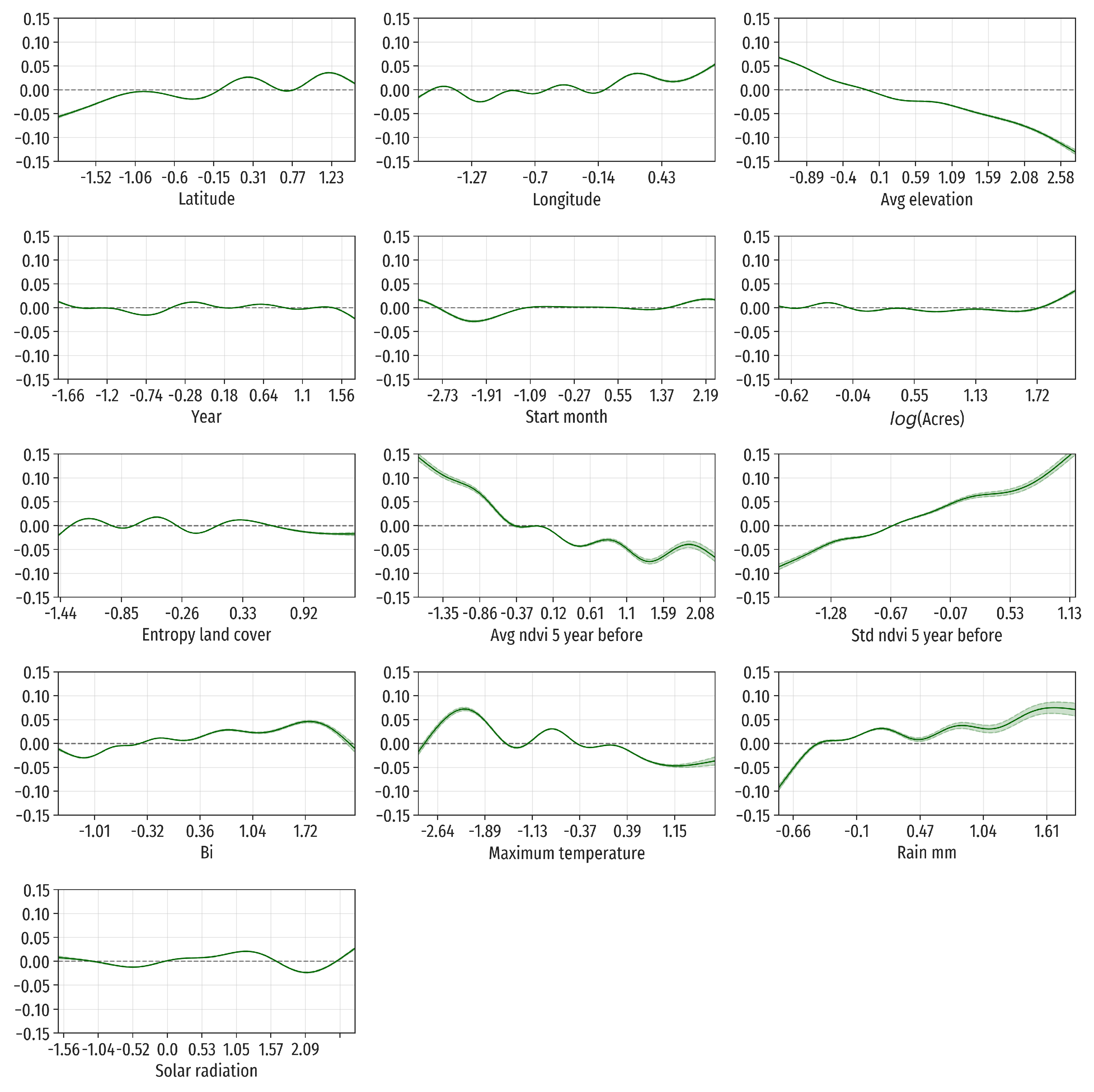
We move our attention now to non-parametrically estimated terms, using the information contained in
Table 4 and in
Figure 7 (showing the estimation of the functional coefficients
) and
Figure 8 (which includes the estimations of the functions
).
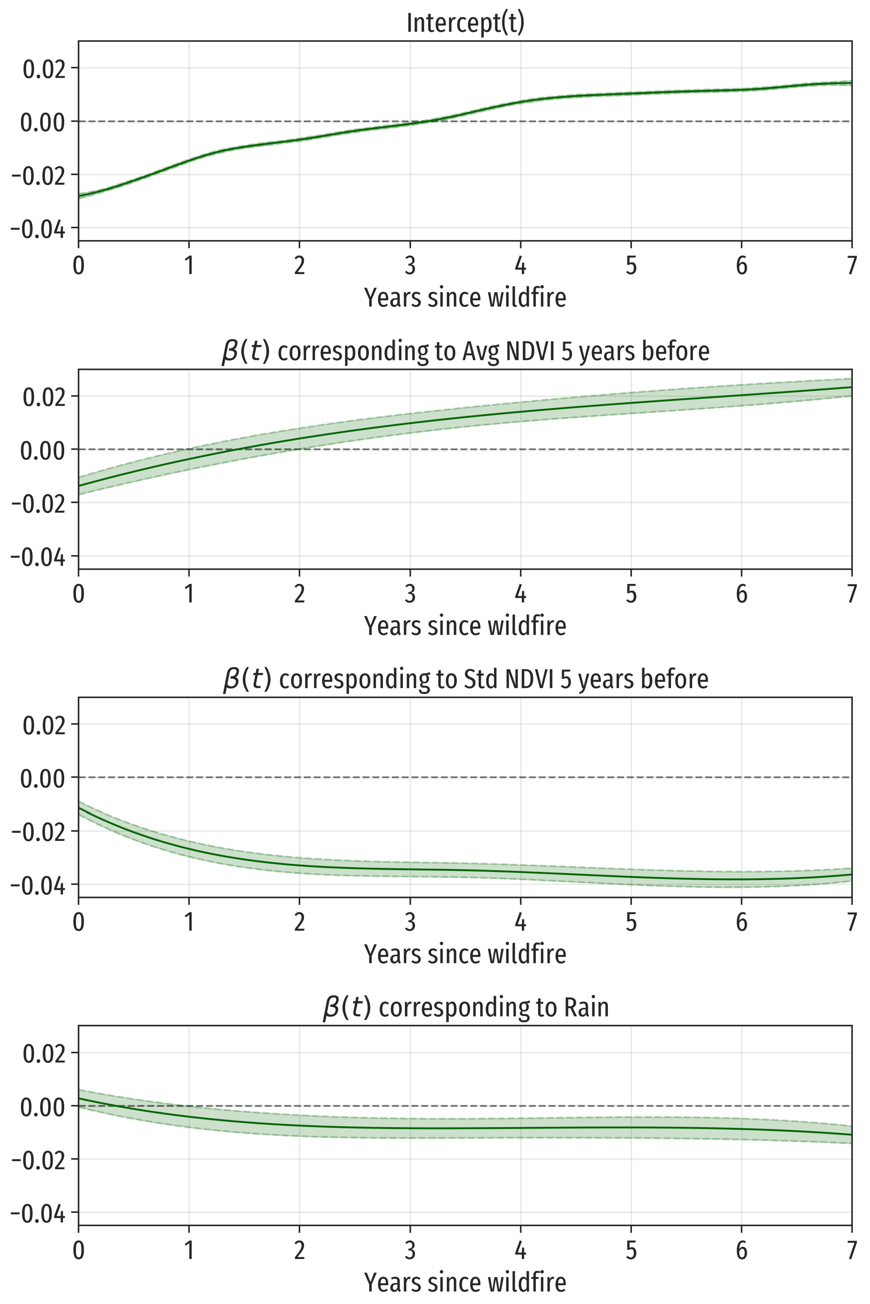
The estimation of the function
in model (
2) is labeled
Intercept(t) in
Figure 7 (upper panel). Except for a vertical shift, it is approximately equal to the mean function (see
Figure 5). The vertical shift should be equal to the estimated
Intercept in
Table 3 if there were no factor covariates in the model. In our case, however, this
Intercept is referred to the level
Evergreen forest of the factor Landcover.
There are three covariates (Avg NDVI 5 years before, Std NDVI 5 years before, and Rain) that contribute with two terms (
and
) to the full additive function-on-scalar model. To understand the contribution of these variables to the response recovery functions, we have to consider simultaneously the two corresponding estimated functions, where one is represented in
Figure 7 and the other one in
Figure 8. Regarding Avg NDVI 5 years before (average of NDVI over the 5 years before the wildfire), the estimation of its functional coefficient
(
Figure 7, second panel) presents a monotonically increasing pattern with a total increment of
NDVI points over the 7 years. At the same time, the estimation of its term
(
Figure 8, third row, second column) is a roughly decreasing function with a range of values of more than
NDVI points. So it follows that the contribution of the term
is much larger than that of the term
for this explanatory variable. The nonparametric term
indicates that larger values of NDVI vegetation tend to suffer more from wildfires. For instance, in average, an area with pre-wildfire NDVI value equal to the mean plus one standard deviation loses
NDVI points more than another area with pre-wildfire NDVI value one standard deviation below the average. For these two fictitious areas, the effect of the term
is to add or subtract, respectively, the estimated coefficient
. Then the area with NDVI values over the mean will have a larger decrease in NDVI the first one and a half yeas, but its recovery will be faster than in the area with previous lower NDVI values.
For Std NDVI 5 years before (standard deviation of NDVI over the 5 years before the wildfire), the relative relevance of the term
is also much smaller than that of the term
: their ranges are
and
, respectively. The functional coefficient
, negative for all
t, is decreasing the first two years and almost constant from then on (with an approximate value of
NDVI points). The term
in this case is an increasing function on the standard deviation of pre-wildfire NDVI values, indicating that vegetation diversity (large values of Std NDVI 5 years before) is a protecting factor against wildfire effects. Combining both terms, the difference in loss of NDVI points between two areas with values of Std NDVI 5 years before one standard deviation over and below the mean, respectively, for
t larger than two years is
For t smaller than 2 years, the differences between these two areas are smaller than and increasing in t.
For the explanatory variable Rain, the term is even less important than in the two previous cases (the range of is smaller than NDVI points, and it is almost constant from two years after the wildfire). On the other hand, the term , that has an approximate range of , grows rapidly at low values of the variable Rain (smaller than times the standard deviation below the mean, approximately) and then it is almost constant or slightly increasing. We conclude that moderate or large precipitations seem to help recover or protect against the wildfire effects.
The remaining 10 explanatory variables contribute to the full additive function-on-scalar model only with a nonparametric term
that remains constant over time after the wildfire. The estimations of these terms are represented in
Figure 8. The most relevant contribution to the model is that of the covariate Avg Elevation, which estimated term
has a range of
NDVI points. This function is decreasing in elevation, indicating that the wildfire effects are larger in more elevated areas, probably because elevated areas present in average richer vegetation (larger pre-wildfire NDVI values) than those with lower elevation.
Less important, although also worth mentioning, are the explanatory variables Bi (burning index) and maximum temperature. For the burning index, the estimated term is an slightly increasing function in the middle part of the range of burning index values. It follows that areas with lower fire hazard will have slightly larger wildfire effects. The estimated term for maximum temperature is roughly decreasing in its argument, indicating that low maximum temperatures protect moderately against the wildfire effects.
Regarding geographical coordinates contribution to the model, the wildfire effects in the South (respectively, West) are larger than in the North (respectively, East), but the differences are small (less than NDVI points).
Lastly, we do not find clear and strong interpretable patterns of dependence between the response, the wildfire effects functions, and the rest of covariates (year, start month, log(acres), entropy land cover, and solar radiation).
The results we have shown indeed provide evidence that function on scalar regression models are a useful methodology to answer the research questions we stated in the introduction. Our findings show that wildfire effects are different depending on the kind of environment (e.g., average elevation of burned areas, average daily accumulated rain or average daily maximum temperatures), and that wildfire effects do vary according to the vegetation of the burned area (i.e., predominant landcover, type of vegetation or greenness of vegetation), as suggested by previous literature [
21,
47,
48,
49,
50,
51]. Our results also suggest that the vegetation response is influenced by the combination of previous conditions of vegetation and climatological characteristics, e.g., we see that environments with vegetation having larger values of NDVI and less seasonal fluctuations are more severely affected. Moreover, the variance in different types of recoveries can be largely explained using pre-wildfire observable covariates, such as weather conditions, greenness, seasonality or location and elevation.
5. Conclusions and Discussion
The functional regression methodology has shown to be an effective way to study and explain vegetation recovery from wildfires, using pre-wildfire explanatory variables. The additive function-on-scalar fitted model explains 72.9% of the total variability of the responses. A large part of the explanatory power of the model goes directly to explain the recovery dynamic through the presence of regression coefficients that change over time. Nevertheless, the main part of the relationship between the explanatory variables and the wildfire effects functions is constant over time after the wildfire and, it is worth mentioning, non-linear.
The most important lessons we draw from this model are the following. On average, the recovery process after a wildfire is slow and takes more than 7 years (the time span used in this study). Each particular wildfire is a combination of a unique set of conditions that alter vegetation and ecosystems in a different manner, and it seems that all of them have an effect on the wildfire recovery process. The main risk conditions for a given area from suffering larger wildfire effects are, in this order, to have a rich and homogeneous vegetation (large and uniform NDVI, dominance of grassland, herbaceous vegetation or evergreen forest as land cover), to present a low precipitation regime, to have a large elevation over the sea level, to have low burning index, to have large maximum temperatures, and to be located in the South or West of California.
The convenience of studying outcomes changing over time, together with the estimation of the effect of several kinds of conditions pre- and post-wildfire, makes functional regression models to be a perfect methodology for this kind of studies. Previous studies use standard multiple regression models to compare absolute values of spectral indices, or comparisons of geolocated rasters such that these can include the spatial component of wildfires. However, giving estimates of the effect of these characteristics on the recovery pattern of vegetation from wildfires will allow environmental scientists and land management entities to study the characteristics that need more preservation.
It is important to notice that this methodology has only been implemented over the recoveries estimated from [
18]. Nevertheless, this could be applied in many other research areas and fields, benefiting from the temporal component that this methodology includes, as everything is observed and measured over time. Expanding the study area to other fire-prone regions around the world, and increasing the time-span observed after wildfires (e.g., 15 years after each fire) would probably allow to observe full recoveries from wildfires. However, this remains outside the scope of this work.
This study tries to close the gap between satellite remote sensing and evaluation of wildfires’ effects over time. It must be noted that gathering and pre-processing data, usually coming from different sources, is a crucial and highly sophisticated task when dealing with remote sensing data. Functional data analysis, and functional regression in particular, is an advanced statistical methodology well suited to analyze such rich data sets.


