Article

On Model Order Reduction of Interconnect Circuit Network: A Fast and Accurate Method

1
Harbin Institute of Technology at Weihai, Weihai 264200, China
2
The School of Aeronautics and Astronautics, Central South University, Changsha 410083, China
3
The School of Electronic and Information Engineering, Harbin Institute of Technology, Shenzhen 518055, China
*
Author to whom correspondence should be addressed.
Mathematics 2021, 9(11), 1248; https://doi.org/10.3390/math9111248
Submission received: 12 May 2021 / Revised: 25 May 2021 / Accepted: 26 May 2021 / Published: 29 May 2021
(This article belongs to the Section Engineering Mathematics)

Abstract

:
The time cost in integrated circuit simulation is an important consideration in the design. This paper investigates the model order reduction of interconnect circuit networks to facilitate numerical analysis. A novel fast and accurate time reduced order model is proposed to simplify the interconnection network structure analysis and perform a fast simulation. The novelty of this study is the use of the power function sum to extend the approximate function to replace the original system’s state function. We give several simulations to verify the effectiveness of the algorithm. The innovation of this model is due to its use of the approximate function of power series expansion to replace the state function of the original system.

1. Introduction

IC (integrated circuit) industry is a crucial link in the development of the information industry, and the development of IC is inseparable from electronic design automation. As the integrated circuit industry evolves, the circuit scale is increasing exponentially [1]. Therefore, in the simulation of the circuit, the modeling of the extraction will be very complex. At the same time, with the continuous reduction of the characteristics of integrated circuit devices, the interconnection delay exceeds the device delay to become the dominant factor in chip performance, and the analysis of interconnection plays an important role in the timing analysis. The question of how to accurately and effectively analyze circuit networks while reducing the simulation time must be urgently addressed [2,3,4]. If a low-order model meeting the error requirements can be derived to replace the original complex model for simulation analysis, then the complexity and simulation time of the simulation will be greatly reduced. This method of deducing the lower-order model to replace the higher-order model is called model reduction. In recent decades, the model order reduction of large circuits and complex systems has been a topic of major interest. For the above-mentioned unavoidable problems in IC progress, it is difficult for traditional simulation tools to effectively analyze VLSI (very large-scale integration) networks.In this context, with the allowable error range, it is expected that the complete interconnect equivalent circuits can be replaced with simpler and more flexible models. In this paper, we use a low-order model to replace the primary large-scale system in practical application, which can dramatically reduce the complexity in analyzing the circuit network structure and maintain the physical characteristic of the primary system [5,6,7,8]. This idea has already received significant attention due to its effective application. Investigations in this area are timely and critical applications to reduce the complexity of systems that, for real application, require suitable reduced-order models, such as systems with distributed models including that used in microfluidics applications [9,10].
The model reduction should satisfy the requirements of accuracy, stability, and low complexity. In fact, nowadays, there are many kinds of methods that can be used to implement model reduction [11,12,13]. Traditional methods to reduce order can be divided into two types: time-domain model reduction [14] and frequency-domain model reduction. Among these, the research on the frequency-domain model reduction method [15,16] is more mature. The most important and fundamental method in frequency-domain model reduction is the Krylov subspace method [8,16,17,18,19,20], and this type of method usually utilizes the orthonormal basis [21] to implement the model reduction. The Krylov subspace method is a type of arithmetic technique, originally developed in the 1950s, which is distinguished by its capacity for solving large-scale linear systems and deriving the eigenvalue of the large-scale matrix [7]. However, for circuit network systems, their time-domain characteristics are becoming increasingly important. The approximate error of the frequency domain with reduced order will be enlarged when it is transformed into the time domain, so it is highly necessary to focus on the time-domain model reduction method and error evaluation method in time-domain model order reduction.
Regarding time-domain model reduction, we propose a new type of order reduction model by using Taylor series approximation theory [22]. With this method, we transform the solution of complex ordinary differential equations of a large interconnection network into the solution of linear equations. Compared with the current time-domain model order reduction methods, the proposed method can reduce the order of the original model and greatly reduce the simulation time while ensuring sufficient accuracy. We make the following contributions in this paper:
(1)
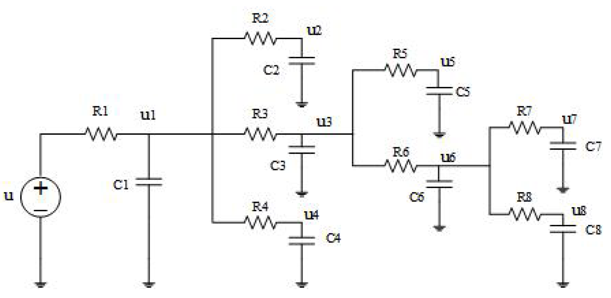
We extract the interconnected parts of the circuit into a network system composed of some different linear elements such as resistors and capacitors.
(2)
We establish the first-order ordinary differential equations of the network system by using state variable analysis.
(3)
By using Taylor series theory, we expand the state variables in the system of differential equations as the sum of the low-order power functions of time t and make the error between the original state variables and the approximately expanded state variables converge.
(4)
We use the norm theory to square the error of each state variable and then integrate it. By limiting the error convergence to the integral interval, the model has a certain error margin. Finally, we take the partial derivative of each of the coefficients and let each of the partial derivatives be equal to zero to minimize the squared error. Both theoretical derivation and simulation results prove that the reduced order model proposed in this paper converges to a certain error limit and can transform the process of solving large ordinary differential equations into the process of solving linear equations. In the time-domain model order reduction, the proposed method is fairly effective in establishing a balance between time-saving and reduced order accuracy.

2. Interconnect Circuit Model

Interconnect networks can be modeled using RL circuit models. To illustrate our method more clearly, we adopt the example of a standard 8-bit adder clock network system (Figure 1). We use Star-RC (which belongs to Synopsys) [23] to extract the resistance and capacitance parameters of the clock network system (we assume that all resistance and capacitance parameters are equal in unit length).
Then, through Kirchhoff’s law, we describe the behavior of a circuit in terms of a set of ordinary differential equations or circuit Equations (1):
u ˙ 1 = u u 1 R C + u 2 u 1 R C + u 3 u 1 R C + u 4 u 1 R C u ˙ 2 = u 1 u 2 R C u ˙ 3 = u 1 u 3 R C + u 5 u 3 R C + u 6 u 3 R C u ˙ 4 = u 1 u 4 R C u ˙ 5 = u 3 u 5 R C u ˙ 6 = u 3 u 6 R C + u 7 u 6 R C + u 8 u 6 R C u ˙ 7 = u 6 u 7 R C u ˙ 8 = u 6 u 8 R C .
The model can be approximated into Equation (2):
X ˙ ( t ) = A X ( t ) + B
where X t R N × 1 denotes the state variable of the node voltage, and N is the number of unknowns in Equation (2). A R N × N denotes the coefficient of the differential equation set determined by the resistance and capacitance parameters. B R N × 1 is the matrix containing the initial value of the node voltage.

3. Order Reduction Method of Approximation Model

3.1. One-Dimensional Convergence Derivation

When the coefficients of the differential equation determined by Equation (2) are one-dimensional (i.e., both matrices A and B are one-dimensional), the matrix A can be simplified to scalar a and the matrix B can be simplified to scalar b. Then, the interconnect model can be simplified to the form X ˙ t = a X t + b . The process of proving the convergence of Equation (2) in the one-dimensional case is as follows:
Expanding X ˙ ( t ) based on Taylor series yields its r order form:
X ( t ) · = a 0 + a 1 t + a 2 t 2 + + a r t r + X ( t ) = a 0 t + 1 2 a 1 t 2 + 1 3 a 2 t 3 + + 1 r + 1 a r t r + 1 + .
The approximate error is R, which can be expressed by Equation (4):
R = X ˙ t a X t b .
Firstly, let r = 2 and obtain 2-norm of the error R in the (5):
Y = 0 T a 0 + a 1 t a a 0 t + 1 2 a 1 t 2 b 2 d t .
From Equation (5), we can see that Y is a multivariate function composed of the expansion coefficient of a 0 , a 1 and the simulation time (i.e., integration interval) T. If the first-order model wishes to converge, the partial derivatives of each parameter must be 0. Since the parameter is independent of the interval, taking the partial derivative of each part of the function Y is equivalent to taking the partial derivative of the part of the integral that has parameters. The expression for the partial derivative of a 0 and a 1 is shown as:
Y a 0 = 2 a 0 T a T 2 + 1 3 a 2 T 3 + 2 a 1 1 2 T 2 1 2 a T 3 + 1 8 a 2 T 4 2 b T 1 2 a T 2 = 0 ,
and
Y a 1 = 2 a 0 1 2 T 2 1 2 a T 3 + 1 8 a 2 T 4 + 2 a 1 1 3 T 3 1 4 a T 4 + 1 20 a 2 T 5 2 b 1 2 T 2 1 6 a T 3 = 0 .
Combining (6) and (7), as T , we can obtain (8):
a 0 1 T + o T , a 1 1 T 2 + o T 2 ,
when r = n 1 and T , we use Gaussian elimination [24] to obtain the results (9),
a 0 1 T + o T , a 1 1 T 2 + o T 2 a n 1 1 T n + o T n .
Under the condition of r = n , using (4) yields the error expression; then, we take its 2-norms and obtain the expression of Y defined in (5). Taking a partial derivative of parameters a 0 , a 1 , a n 1 , a n in Y, we thus obtain n + 1 linear algebraic equations. Using the aforementioned method, e.g., if r = 2 , we can solve the same n + 1 equations. When we solve these equations, firstly, we consider a n a constant and then obtain the parameter a 0 , a 1 , a n 1 . The result is given as:
a 0 T n + o T n a n , a 1 T n 1 + o T n 1 a n a n 1 T 1 + o T 1 a n .
Thus, we can draw the conclusion that, under one-dimensional circumstances, the approximation model order reduction of (2) is convergent.

3.2. Two-Dimensional Convergence Derivation

X ˙ t = A X t + B under the two-dimensional condition:
A = m 11 m 12 m 21 m 22 , B = b 1 b 2 .
This condition is on behalf of the universality of the derivation in multidimensional cases. X ˙ t = f 1 t f 2 t , X t = F 1 t F 2 t is given in (12), respectively.
f 1 t = a 10 + a 11 t + a 12 t 2 + + a 1 r t r f 2 t = a 20 + a 21 t + a 22 t 2 + + a 2 r t r F 1 t = a 10 t + 1 2 a 11 t 2 + 1 3 a 12 t 3 + + 1 r + 1 a 1 r t r + 1 F 2 t = a 20 t + 1 2 a 21 t 2 + 1 3 a 22 t 3 + + 1 r + 1 a 2 r t r + 1
where the constant part of F 1 t , F 2 t is absorbed by matrix B in (2). Similar to the one-dimensional circumstance, we obtain errors Δ f 1 , Δ f 2 , respectively, and then take the 2-norms, which yields the expression in (13):
Y = 0 T Δ f 1 2 + Δ f 2 2 d t .
Take the partial derivative of each coefficient in Y, respectively, and make all partial derivatives equal to 0; then, one obtains 2 r + 1 equations. Under the precondition that T , the equation can be simplified, and we obtain Δ f 1 = f 1 t m 11 F 1 t m 12 F 2 t b 1 . Substituting (11) into Δ f 1 , we obtain (14):
Δ f 1 = a 10 + a 11 t + a 12 t 2 + + a 1 r t r m 11 a 10 t + 1 2 a 11 t 2 + 1 3 a 12 t 3 + + 1 r + 1 a 1 r t r + 1 m 12 a 20 t + 1 2 a 21 t 2 + 1 3 a 22 t 3 + + 1 r + 1 a 2 r t r + 1 b 1 Y = 0 T Δ f 1 2 + Δ f 2 2 d t .
Similar to the simplification above, because f 1 t has a lower order in t than F 1 t , the f 1 t can be ignored. We thus obtain the simplified formula (15):
Δ f 1 m 11 F 1 t m 12 F 2 t b 1 Δ f 2 m 21 F 1 t m 22 F 2 t b 2 Δ f 1 a 10 = 1 m 11 t m 11 t Δ f 2 a 10 = m 21 t .
Combining (11) to (15) and taking the outcome above into the integration Equation (13), we obtain the general term Y a 1 k and Y a 2 k in (16) and (17).
Y 2 a 1 k = Δ f 1 Δ f 1 a 1 k + Δ f 2 Δ f 2 a 1 k = m 11 2 + m 21 2 1 k + 3 a 10 T + 1 k + 4 1 2 a 11 T 2 + + m 11 2 + m 21 2 1 k + r + 3 1 r + 1 a 1 r T r + 1 + m 11 m 12 m 21 m 22 1 k + 3 a 20 T + 1 k + 4 1 2 a 21 T 2 + + m 11 m 12 m 21 m 22 + 1 k + r + 3 1 r + 1 a 2 r T r + 1 + 1 k + 2 b 1 m 11 + b 2 m 21 = 0 ,
and
Y 2 a 2 k = Δ f 1 Δ f 1 a 2 k + Δ f 2 Δ f 2 a 2 k = m 11 m 12 + m 21 m 22 1 k + 3 a 10 T + + m 11 m 12 + m 21 m 22 1 k + r + 3 1 r + 1 a 1 r T r + 1 + m 11 2 + m 21 2 1 k + 3 a 20 T + 1 k + 4 1 2 a 21 T 2 + + m 11 2 + m 21 2 1 k + r + 3 1 r + 1 a 2 r T r + 1 + 1 k + 2 b 1 m 12 + b 2 m 22 = 0
where ( k = 0 , 1 , 2 , , r ) . By the fundamental theorem of algebra, we know that this equation has 2 ( r + 1 ) solutions. The universal Formula (16) shows that a 2 r T r + 1 should be equivalent to a constant if this model is convergent when T . Therefore, if the order of a 2 r in the denominator is greater than T r + 1 , the product term tends towards zero. At the same time, because the number of equations is greater than the number of variables, the equation has no solution.
Furthermore, if the order of a 2 r is less than T r + 1 , the product goes to infinity. Correspondingly, the order of a 2 r must be equal to T r + 1 . The expression of each coefficient is given by (18):
a 10 1 T + o T , a 11 1 T 2 + o T 2 a 1 r 1 T r + 1 + o T r + 1 a 20 1 T + o T a 21 1 T 2 + o T 2 a 2 r 1 T r + 1 + o T r + 1 .

3.3. N-Dimensional Convergent Derivation

In order to prove the generality of the model—that is, that formula (2) converges—we need to extend the model to the N dimensions. Firstly, the N-dimensional expansion of Equation (2) is carried out, as shown in Equation (19):
f 1 t f 2 t f n t = m 11 m 12 m 21 m 22 m 1 n m 2 n m n 1 m n 2 m n n · F 1 t F 2 t F n t + b 1 b 2 b n .
Then, as before, we take the 2-norm of the error vector, and we obtain the squared error:
Y = 0 T Δ f 1 2 + Δ f 2 2 + Δ f n 2 d t .
Then, analogous to the case in two dimensions, we use Equation (21) to calculate the general term of Y a h k . Finally, n r + 1 equations are obtained from Equation (21), which contains n r + 1 unknown variables. According to the two-dimensional derivation of r order of a i j T j + 1 , a i j has the form T j + 1 + o T j in the denominator, where the order of o T j is less than the highest order of a i j using j + 1 ,
Y a h k = i = 1 n m 1 h m 1 i j = 0 r 1 k + j + 3 1 j + 1 a i j T j + 1 + i = 1 n m 2 h m 2 i j = 0 r 1 k + j + 3 1 j + 1 a i j T j + 1 + + i = 1 n m n h m n i j = 0 r 1 k + j + 3 1 j + 1 a i j T j + 1 + i = 1 n b i m i h 1 k + 2 = 0
where k = 0 , 1 , 2 , , r h = 1 , 2 , , n . In other words, if the highest order of a i j in the denominator is greater than T j + 1 , then a i j T j + 1 is equal to zero as T . At the same time, because the number of the system is larger than the number of unknown variables in the system, there is no solution. Conversely, if the highest order of a i j in the denominator is less than T j + 1 , then, as T , the product of a i j T j + 1 also goes to infinity. From this, we know that the highest order of a i j in the denominator is T j + 1 ; then, the general solution is given as:
a h k 1 T k + 1 + o T k + 1
where k = 0 , 1 , 2 , ; r h = 1 , 2 , , n . In general, in the n-dimensional, the approximate expands of X ˙ t = A X t + B after order reduction has an expansion coefficient, which makes the formula converge. If so, bring the required coefficient into (19), and the average error limit of approximating reduced order can be calculated by dividing the result by the integral interval T.

4. Simulation Results and Analysis

4.1. Simple Model Implementation

Based on the above derivation, we expand the state variable X in the form of a power function sum and calculate the expansion coefficient. Firstly, we establish a set of n-dimensional and r order equations according to the derivation of Equation (21). From this, it can be seen that the form of the system to be solved is C Q + D = 0 , where Q is the column matrix composed of expansion coefficients, C is the model coefficient, and D is the constant matrix containing the initial parameters. Let n = 2 , r = 2 , and then give the initial voltage value in (2) to yield the column matrix B. The matrix form of A is m 11 m 12 m 21 m 22 . The matrix form of M T , which is from (21) and is related to the integral interval T, is shown in (23):
M T = T 1 1 × 3 T 2 2 × 4 T 1 1 × 4 T 2 2 × 5 .
The optimal solution of matrix M T can be obtained by a reasonable choice of the parameter T. We use a simulated evolutionary algorithm to find the best value for T. The simulated evolutionary algorithm is essentially a class of random search algorithm based on the simulation of the biological evolution process. Its basic idea can be summarized as follows:
(1)
The objective function to be optimized can be understood as the adaptability of a biological population to the environment.
(2)
The optimization variable corresponds to the individual of the biological population.
(3)
Analogize the problem that needs to be optimized with the evolution of a population.
The form of the M-matrix is shown in Equation (24), which is generated by Equation (21) and is the product of the coefficient matrix A of the system of ordinary differential equations and the transpose of A.
M = A × A T = M 11 M 12 M 21 M 22 .
We know that the coefficient matrix C is a matrix with four rows and four columns. In addition, according to Equation (21) and our knowledge of matrix theory, the form of matrix C is the Kronecker product of the matrix M and matrix M T deduced above:
C = M M T = M 11 × M T M 12 × M T M 21 × M T M 22 × M T
Similarly, we can obtain the constant matrix D. Thus, the matrix equation can be solved, in which the coefficients of the state variables of the equation are decomposed into the form of a power series sum. In addition, the system value of each moment can be easily calculated.

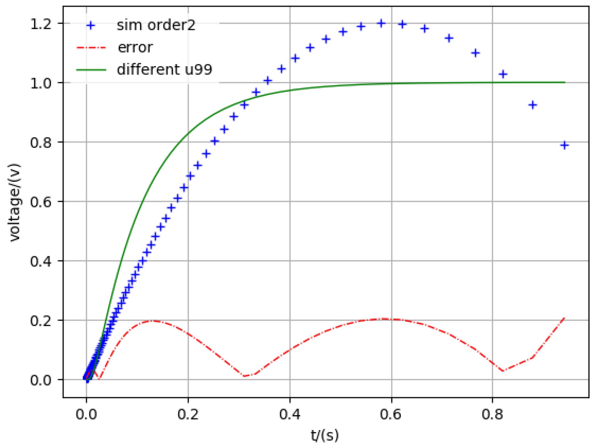
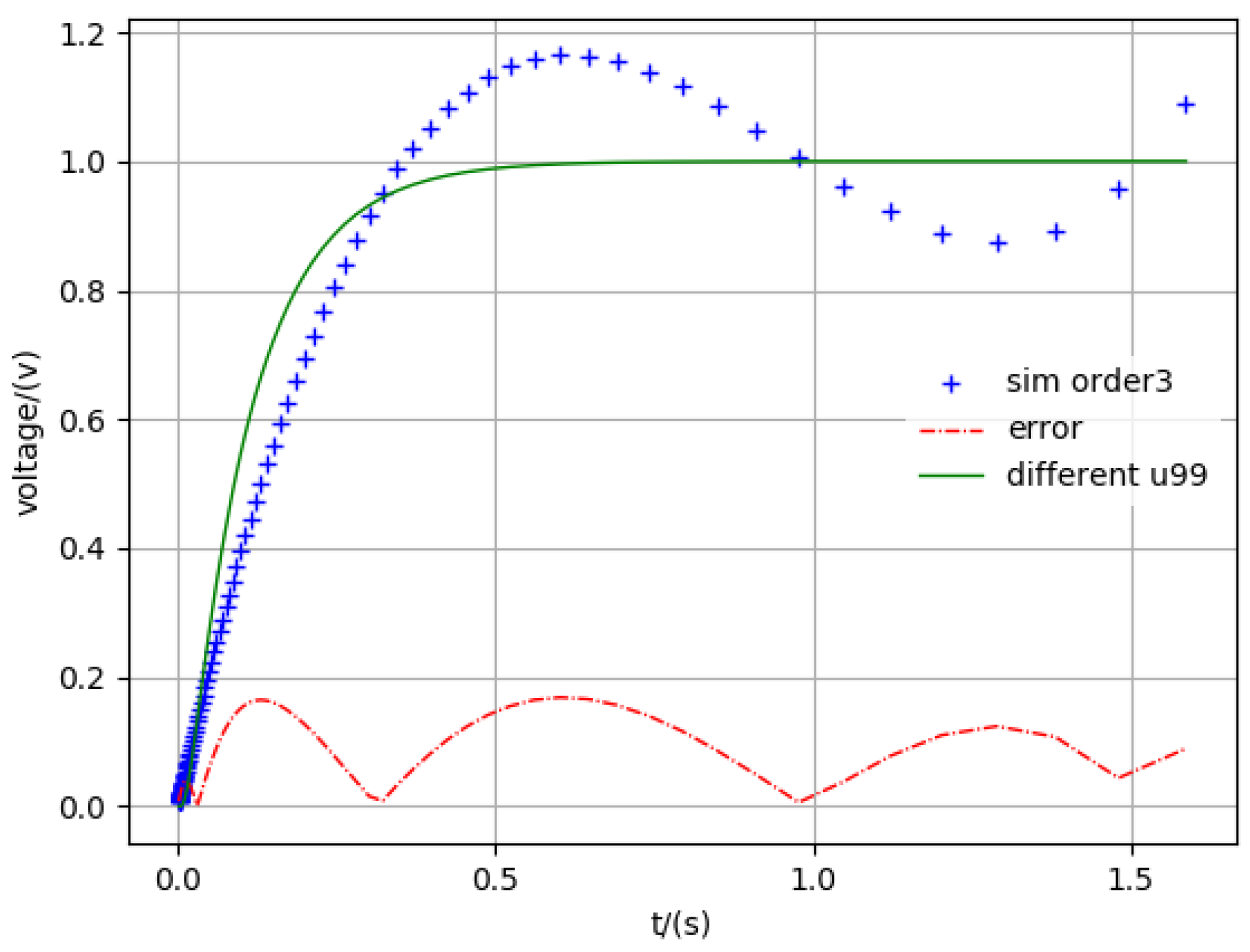
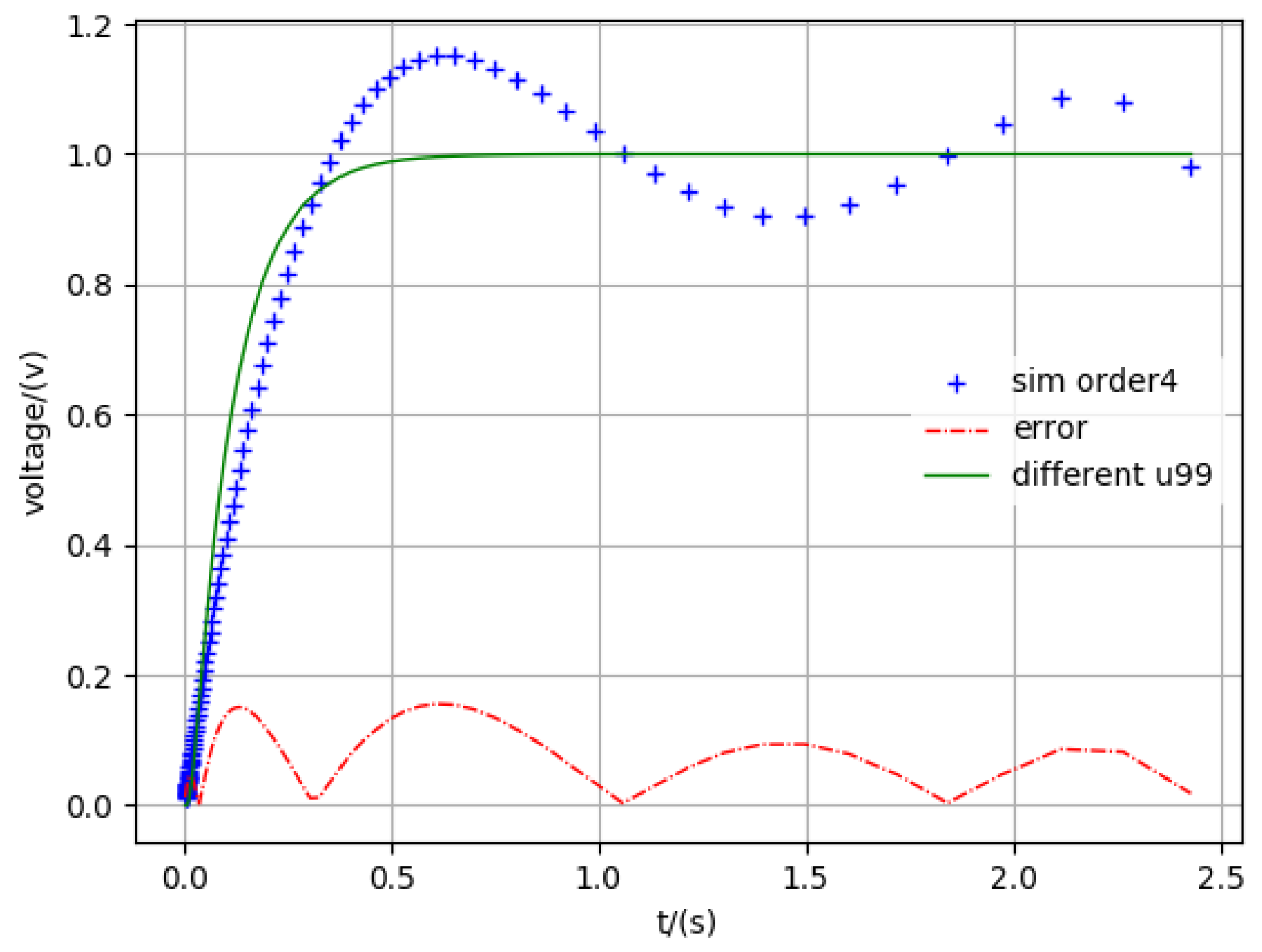
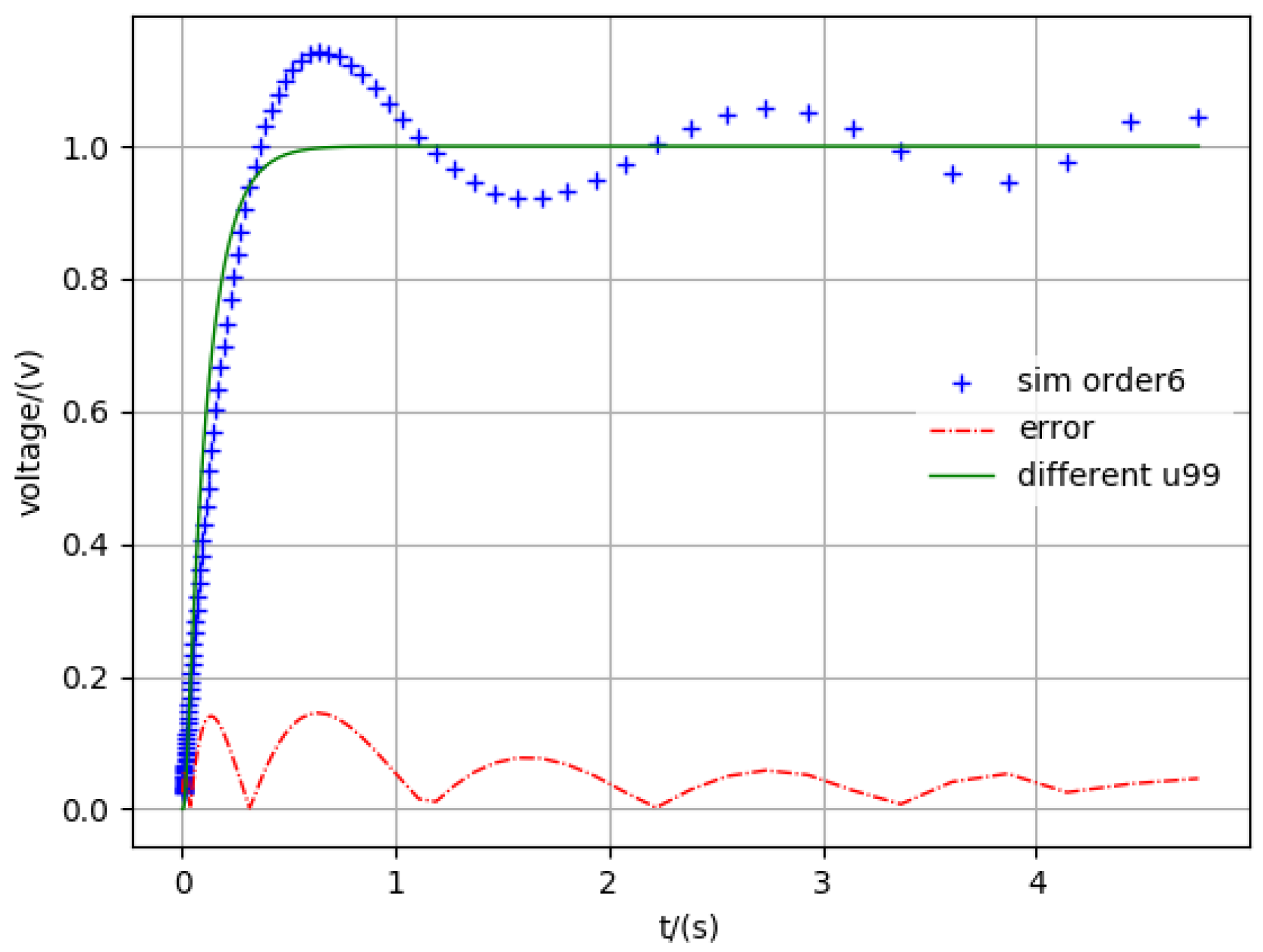
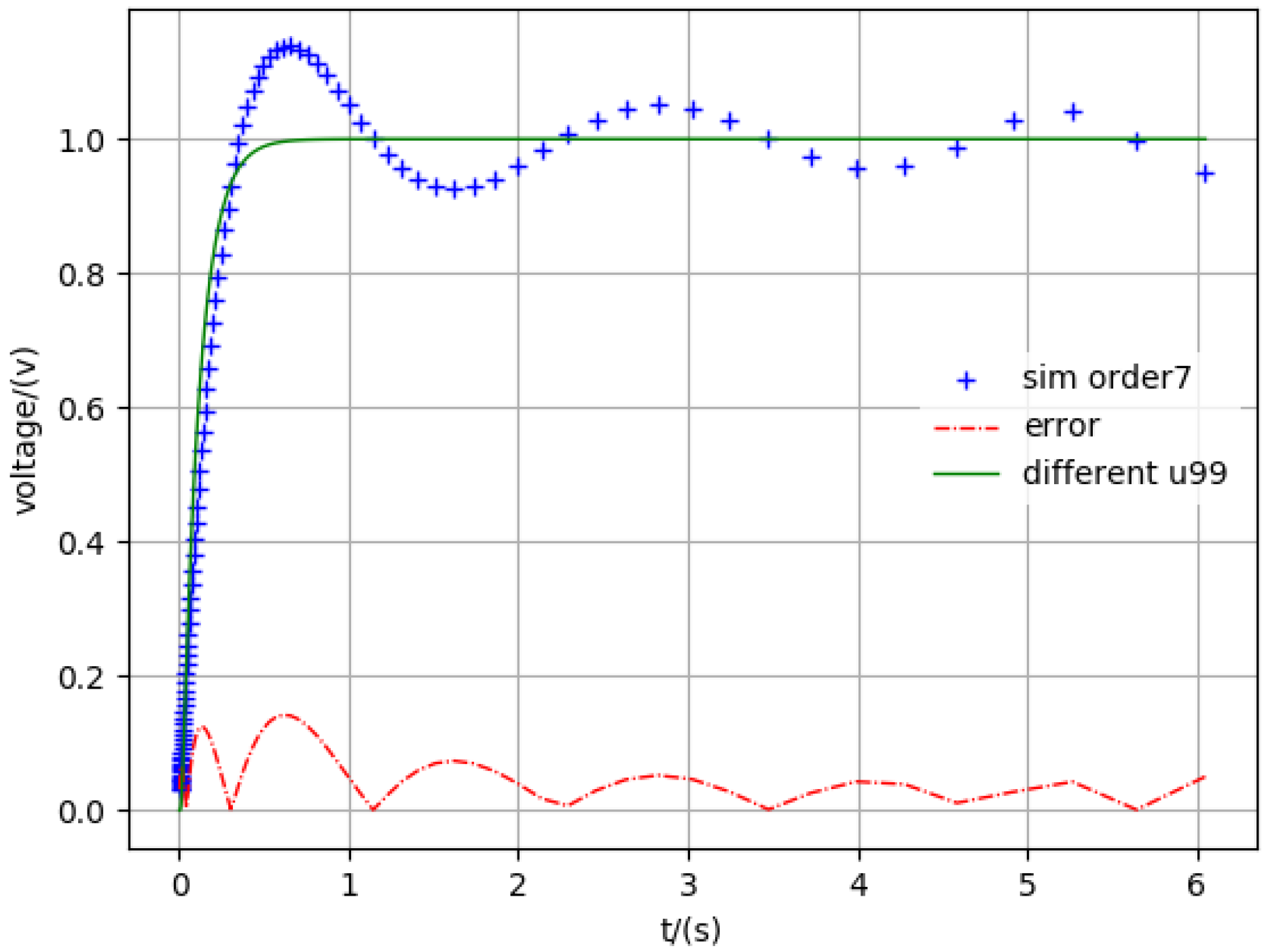
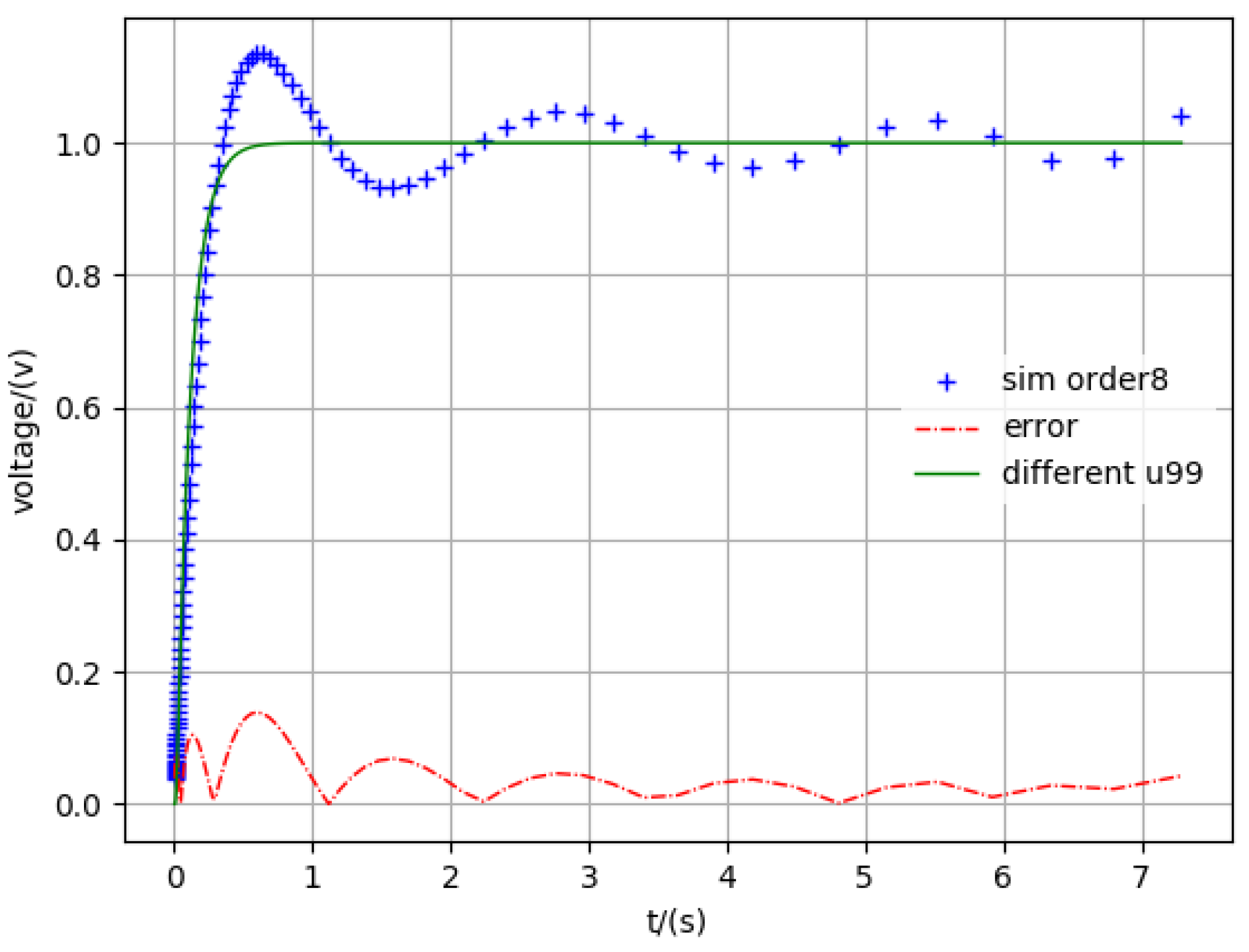
4.2. Model Example and Simulation Results

To verify the model order reduction algorithm proposed in this paper, we arbitrarily selected a clock network. Figure 2 shows a clock network structure with 100 nodes extracted from the actual circuit, where each black dot represents a capacitor and a resistor. The resistance value, capacitance value, and voltage value extracted by the STAR-RC tool were 1.51, 3.8410-4pF, and 1 V. The equations representing linear time-invariant circuit systems are X ˙ t = A X t + B . We performed the matrix processing by using the Numpy extension library in Python, and we drew the images using the Matplotlib extension library. We obtained Table 1 from the Matplotlib plot. Table 1 shows the running time and error margin of the order reduction model proposed in this paper under different degrees of order reduction. As can be seen from Table 1, the order reduction method proposed in this paper can effectively reduce the solution time, and the error is so small that it can be ignored. Figure 3, Figure 4, Figure 5, Figure 6, Figure 7, Figure 8, Figure 9 and Figure 10 show the simulation results under different order reductions.
The legend “different u99” in all figures is the 99th node voltage in Figure 2, which includes a total of 100 nodes. The “sim order*” means the simulation results in different reduced order. The “error” shows the difference between the accuracy results and different reduced orders. From these figures, we can also see that the method proposed in this paper is accurate.
In addition, with the increase in order, the solution of the reduced order will approximate the exact one. This result proves that the order reduction method proposed in this paper is generally applicable to large interconnect lines. The order reduction method proposed in this paper can also adjust the simulation time and simulation precision according to the specific needs. Therefore, based on the above example analysis, we can conclude that the order reduction method can effectively reduce the simulation time, and the error converges to a certain error margin in any time range.

5. Conclusions

In this paper, a novel method of order reduction in the time domain is proposed. Compared with the existing time-domain order reduction models, the proposed method does not need the conversion from the frequency domain to the time domain and improves the stability. By combining the Taylor series and norm, the method can greatly reduce the time and space complexity by transforming the differential equation into a linear equation. The method has proven to be effective and reasonable by extracting the mathematical model of the specific integrated circuit and combining it with mathematical means. The simulation results show that the order reduction method proposed in this paper has the advantages of low computational cost, high precision, and a certain error margin, and it can be applied to the simulation of large interconnects. At the same time, we can also clearly see that with the increase in the model order, the model’s result is closer to the exact solution. Therefore, we can compromise the choice of running time and model order according to the need for precision. In addition, the simplified method mainly introduces the error at the initial time, so the error limit can be further reduced by optimizing the design.

Author Contributions

Funding acquisition, X.W.; Methodology, X.W.; Supervision, X.W.; Validation, S.F.; Writing—original draft, S.F.; Writing—review & editing, M.-Z.D. and C.Z. All authors have read and agreed to the published version of the manuscript.

Funding

This research was funded by Shandong Province Natural Science Foundation (ZR2020KF016) and National Natural Science Foundation of China (Grant Number 62003112).

Institutional Review Board Statement

Not applicable.

Informed Consent Statement

Not applicable.

Data Availability Statement

Not applicable.

Conflicts of Interest

The authors declare no conflict of interest.

References

  1. Lithotechsolutions. Current Status of the Integrated Circuit Industry in China. J. Microelectron. Manuf. 2018, 1, 1–8. [Google Scholar]
  2. Telescu, M.; Tanguy, N.; Bréhonnet, P.; Vilbé, P.; Calvez, L.C.; Huret, F. Model-order reduction of VLSI circuit interconnects via a Laguerre representation. In Proceedings of the 9th IEEE Workshop on Signal Propagation on Interconnects, Garmisch-Partenkirchen, Germany, 10–13 May 2005; pp. 107–110. [Google Scholar]
  3. Achar, R.; Nakhla, M.S. Simulation of high-speed interconnects. Proc. IEEE 2001, 89, 693–728. [Google Scholar] [CrossRef] [Green Version]
  4. Li, P.; Shi, W. Model order reduction of linear networks with massive ports via frequency-dependent port packing. In Proceedings of the 43rd Annual Design Automation Conference, San Francisco, CA, USA, 24–28 July 2006; pp. 267–272. [Google Scholar]
  5. Scarciotti, G. Steady-State Matching and Model Reduction for Systems of Differential–Algebraic Equations. IEEE Trans. Autom. Control. 2017, 62, 5372–5379. [Google Scholar] [CrossRef] [Green Version]
  6. Fujimoto, K. On subspace balanced realization and model order reduction for nonlinear interconnected systems. In Proceedings of the 2012 IEEE 51st IEEE Conference on Decision and Control (CDC), Maui, HI, USA, 10–13 December 2012; pp. 4314–4319. [Google Scholar]
  7. Yan, B.; Zhou, L.; Tan, S.X.D.; Chen, J.; McGaughy, B. DeMOR: Decentralized model order reduction of linear networks with massive ports. In Proceedings of the 45th annual Design Automation Conference, Anaheim, CA, USA, 9–13 June 2008; pp. 409–414. [Google Scholar]
  8. Tan, S.X.D.; Yan, B.; Wang, H. Recent Advance in Non-Krylov Subspace Model Order Reduction of Interconnect Circuits. Tsinghua Sci. Technol. 2010, 15, 151–168. [Google Scholar] [CrossRef]
  9. Cairone, F.; Gagliano, S.; Carbone, D.C.; Recca, G.; Bucolo, M. Micro-optofluidic switch realized by 3D printing technology. Microfluid. Nanofluidics 2016, 20, 61. [Google Scholar] [CrossRef]
  10. Anandan, P.; Gagliano, S.; Bucolo, M. Computational models in microfluidic bubble logic. Microfluid. Nanofluidics 2015, 18, 305–321. [Google Scholar] [CrossRef]
  11. Gunupudi, P.; Khazaka, R.; Dounavis, A.; Nakhla, M.; Achar, R. Global multi-level reduction technique for nonlinear simulation of high-speed interconnect circuits. In Proceedings of the IEEE 10th Topical Meeting on Electrical Performance of Electronic Packaging (Cat. No. 01TH8565), Cambridge, MA, USA, 22–31 October 2001; pp. 259–262. [Google Scholar]
  12. Papachristodoulou, A.; Chang, Y.C.; August, E.; Anderson, J. Structured model reduction for dynamical networked systems. In Proceedings of the 49th IEEE Conference on Decision and Control (CDC), Atlanta, GA, USA, 15–17 December 2010; pp. 2670–2675. [Google Scholar]
  13. Choroszucha, R.B.; Sun, J. Empirical Riccati covariance matrices for closed-loop model order reduction of nonlinear systems by balanced truncation. In Proceedings of the 2017 American Control Conference (ACC), Seattle, WA, USA, 24–26 May 2017; pp. 3476–3482. [Google Scholar]
  14. Xu, Q.; Li, Z.F.; Mazumder, P.; Mao, J.F. Time-domain modeling of high-speed interconnects by modified method of characteristics. IEEE Trans. Microw. Theory Tech. 2000, 48, 323–327. [Google Scholar]
  15. Ding, W.; Liu, F.; Liu, S.; Wang, G. Localization of critical frequency for simulation of high-speed interconnects. In Proceedings of the 2014 15th International Conference on Electronic Packaging Technology, Chengdu, China, 12–15 August 2014; pp. 1512–1515. [Google Scholar]
  16. Sun, Y.; Dong, J.; Pu, T.; Yu, T. Reduction of power system dynamic model using Krylov subspace method. In Proceedings of the 2014 International Conference on Power System Technology, Chengdu, China, 20–22 October 2014; pp. 343–348. [Google Scholar]
  17. Zhu, Z.; Geng, G.; Jiang, Q. Power System Dynamic Model Reduction Based on Extended Krylov Subspace Method. IEEE Trans. Power Syst. 2016, 31, 4483–4494. [Google Scholar] [CrossRef]
  18. Chaniotis, D.; Pai, M. Model reduction in power systems using Krylov subspace methods. IEEE Trans. Power Syst. 2005, 20, 888–894. [Google Scholar] [CrossRef] [Green Version]
  19. Frangos, M.; Jaimoukha, I. Adaptive rational Krylov algorithms for model reduction. In Proceedings of the 2007 European Control Conference (ECC), Kos, Greece, 2–5 July 2007; pp. 4179–4186. [Google Scholar]
  20. Chen, Y.; Balakrishnan, V.; Koh, C.K.; Roy, K. Model Reduction in the Time-Domain Using Laguerre Polynomials and Krylov Methods. In Proceedings of the 2002 Design, Automation and Test in Europe Conference and Exhibition, Paris, France, 4–8 March 2002; pp. 931–935. [Google Scholar]
  21. Jiang, G.; Liu, H.; Yang, K.; Gao, X. A fast reduced-order model for radial integral boundary element method based on proper orthogonal decomposition in nonlinear transient heat conduction problems. Comput. Methods Appl. Mech. Eng. 2020, 368, 113190. [Google Scholar] [CrossRef]
  22. Panjapornpon, C.; Kajornrungsilp, I.; Rochpuang, C. Input/output linearizing controller with Taylor series expansion for a nonminimum phase process by hardware-in-the-loop approach. Asia-Pac. J. Chem. Eng. 2020, 15, e2440. [Google Scholar] [CrossRef]
  23. Hsinchu. Synopsys and UMC Collaborate to Accelerate Development of a 14nm Finfet Process. Electron. World 2013, 119, 50. [Google Scholar]
  24. Geng, X.; Xiao, Z.; Ji, L.; Zhao, Y.; Wang, F. A Gaussian elimination based fast endmember extraction algorithm for hyperspectral imagery. ISPRS J. Photogramm. Remote Sens. 2013, 79, 211–218. [Google Scholar] [CrossRef]
Figure 1. Clock network structure of an 8-bit adder system.
Mathematics 09 01248 g001
Figure 2. Structure of clock network.
Mathematics 09 01248 g002
Figure 3. Simulation second-order.
Mathematics 09 01248 g003
Figure 4. Simulation three-order.
Mathematics 09 01248 g004
Figure 5. Simulation four-order.
Mathematics 09 01248 g005
Figure 6. Simulation five-order.
Mathematics 09 01248 g006
Figure 7. Simulation six-order.
Mathematics 09 01248 g007
Figure 8. Simulation seven-order.
Mathematics 09 01248 g008
Figure 9. Simulation eight-order.
Mathematics 09 01248 g009
Figure 10. Simulation nine-order.
Mathematics 09 01248 g010
Table 1. The running time and margin of error in different orders.
Reduced OrderTime (s)Average Error Margin
20.038567 s0.208194
30.090528 s0.168275
40.172582 s0.154782
50.252482 s0.148063
60.358407 s0.144806
70.463968 s0.142452
80.637438 s0.141266
90.739400 s0.140600
exact solution12.165914 s0
Publisher’s Note: MDPI stays neutral with regard to jurisdictional claims in published maps and institutional affiliations.

