Article

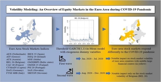
Volatility Modeling: An Overview of Equity Markets in the Euro Area during COVID-19 Pandemic

by
Pierdomenico Duttilo
*,
Stefano Antonio Gattone
and
Tonio Di Battista
DISFIPEQ, University “G. d’Annunzio” of Chieti-Pescara, 65127 Pescara, Italy
*
Author to whom correspondence should be addressed.
Mathematics 2021, 9(11), 1212; https://doi.org/10.3390/math9111212
Submission received: 24 March 2021 / Revised: 16 May 2021 / Accepted: 21 May 2021 / Published: 27 May 2021

Abstract

:
Volatility is the most widespread measure of risk. Volatility modeling allows investors to capture potential losses and investment opportunities. This work aims to examine the impact of the two waves of COVID-19 infections on the return and volatility of the stock market indices of the euro area countries. The study also focuses on other important aspects such as time-varying risk premium and leverage effect. This investigation employed the Threshold GARCH(1,1)-in-Mean model with exogenous dummy variables. Daily returns of the euro area stock markets indices from 4 January 2016 to 31 December 2020 has been used for the analysis. The results reveal that euro area stock markets respond differently to the COVID-19 pandemic. Specifically, the first wave of COVID-19 infections had a notable impact on stock market volatility of euro area countries with middle-large financial centres while the second wave had a significant impact only on stock market volatility of Belgium.

Graphical Abstract

1. Introduction

Volatility is a measure of financial risk or uncertainty of equity portfolios. The degree of vulnerability of stock market indices to global financial crisis is a key factor which can help portfolio managers in optimizing their investment decisions [1,2,3]. The aim of this work is to evaluate the impact of COVID-19 pandemic on the return and volatility of equity markets in the euro area countries.
The first COVID-19 infections were identified in Wuhan city, Hubei province of China in December 2019. On 21 February 2020, Northern Italy registered a significant increase of COVID-19 cases, while other European states started to report cases of infected people [4]. Later, on 11 March 2020, the World Health Organization (WHO) declared COVID-19 a pandemic [5].
The continuous spread of the novel coronavirus has wide effects on national economies and financial markets across the world. Figure 1 shows the Gross Domestic Product (GDP) growth rates compared to the same quarter of previous year in the euro area (EA), European Union (EU) and North American Free Trade Agreement (NAFTA) from 1st quarter 2016 to 4th quarter 2020. During the last quarter of 2020, GDP decreased by 5.01 % in the EA, 4.75 % in the EU and 2.80 % in the NAFTA compared with the last quarter of 2019. Probably due to containment measures of Covid-19, the worst peak occurred in the 2nd quarter 2020 (− 14.71 % in the EA, − 13.89 % in the EU and − 10.26 % in the NAFTA) [6]. According to International Monetary Fund’s January 2021 World Economic Outlook (WEO), the euro area growth contraction for 2020 is estimated at − 7.2 % [7]. These poorly economics performance have led to a “bearish stock market” [8] and “financial market turmoil” [9]. For instance, the closing prices of Euro Stoxx 50 Index and S&P 500 Index show a sharp drop in the first quarter of 2020 (Figure 2, red areas). Additionally, Figure 2 highlights a rapid recovery of S&P 500 and a slow recovery of Euro Stoxx 50 during other quarters. Equally important is the high level of volatility, on 16 March 2020, CBOE Volatility Index (VIX) [10] closed at 82.69, surpassing the peak level of 80.86 on 20 November 2008 [11]. As showed by Just and Echaust (2020) [12] there is a close dependece between US stock market returns (S&P 500) and implied volatility (VIX).
Volatility is a key factor of financial markets, it is a measure of financial risk or uncertainty of financial assets [13]. According to Bhowmik and Wang (2020) [1] there is a direct relationship between volatility and market uncertainty. Therefore, volatility affects “the investment behavior of enterprises and individuals” [1] providing a tool to predict the market behaviour [14]. For istance, Di Persio et al. (2021) [14] implement a volatility target strategy using a hybrid algorithm based on GARCH model and Neural Network (NN) approach.
No study so far has examined the differential impact of coronavirus health crisis with specific focus on the European stock markets. Euro-area members share the same currency (€) and monetary policy, but at the same time they differ by financial centers size (i.e., Real GDP per capita and stock market capitalization) and other features such as financial culture, risk aversion, population age, trades (export vs oriented economies) and so on. Using the GARCH modeling approach, the purpose of this paper is to analyse the impact of the COVID-19 pandemic on returns and volatility of the stock market indices of the euro area countries. We consider the daily returns over the period from 4 January 2016 to 31 December 2020 of the following indices: AEX (the Netherlands), ATF (Greece), ATX (Austria), BEL 20 (Belgium), CAC 40 (France), CYMAIN (Cyprus), DAX (Germany), FTSE MIB (Italy), IBEX 35 (Spain), ISEQ 20 (Ireland), MSE (Malta), OMXBBPI (the Baltic states of Estonia, Latvia, and Lithuania), OMXH 25 (Finland), PSI 20 (Portugal), SAX (Slovakia) and SBITOP (Slovenia). In particular, the effect of COVID-19 pandemic is captured through two exogenous dummy variables reflecting the two main waves of COVID-19 infections.
Our findings show that euro area stock markets respond differently to the COVID-19 pandemic, euro-area members with small financial centers appear to be more resilient to COVID-19 compared to euro-area members with middle-large financial centers. For the latter, the first wave of COVID-19 infections had a significant impact on the stock market volatility. Furthermore, we find that almost all euro area countries show a weakening of the impact of COVID-19 as the crisis evolved.
The rest of the paper is organized as follows. Section 2 includes the literature review. Section 3 describes the methodology and the data used. Section 4 illustrates the results of the analysis. Finally, Section 5 provides the results discussion and some conclusions.

2. Literature Review

2.1. Impact of Older Global Crises on Stock Market Volatility

There is a considerable amount of research devoted to the vulnerability of stock markets during global crises. Using a nonparametric quantiles-based model Goswami et al. (2020) [15] stated that global crises have a stronger impact on market volatility than domestic crises. Specifically, the authors take into account different type of crises such as: banking crises, inflation crises, currency crises, stock market crashes, external and domestic sovereign debt crises [15]. Singhania and Anchalia (2013) [16] examined the impact of global crisis (sub-prime crisis of 2008 and European debt crisis) on volatility of Asian stock markets returns: India (Nifty), China (Shanghai Composite), Hong Kong (Hang Seng) and Japan (Nikkei 225). Their findings show that sub-prime crisis impacted positively the volatility of the Japanese, Chinese and Indian stock markets.
There are other important features of volatility such as persistence and leverage effect that could be affected by global crises. For instance, according to Angabini and Wasiuzzaman (2011) [17] the 2008 global financial crisis led to a “small drop in persistence” [17] and a “significant increase in volatility and leverage effect” [17] of the KLCI Index (Malaysian Stock Market). Okičić (2015) [18] identified the existence of a leverage effect in Central and Eastern Europe (CEE) stock markets using ARIMA and GARCH processes.
Ahmad et al. (2014) examined “The Eurozone crisis and its contagion effects on the European stock markets” [19] through the dynamic conditional correlation GARCH model (DCC-GARCH). With regard to volatility, their empirical results suggest that Greece showed the highest volatility among euro area countries during the Eurozone crisis period (from 19 October 2009 to 31 January 2012). Additionally, Greece was followed by Italy, Spain and Austria [19]. Zhu et al. (2019) [20] analysed the impact of the 2008 global financial crisis on seven Latin American stock markets. They argued that investors prefer to invest in the post-crisis period because stock markets are less volatile.

2.2. Impact of COVID-19 Pandemic on Stock Market Volatility

The impact of the novel coronavirus on stock markets has been the topic of several empirical studies. Using an event study method, HaiYue Liu et al. [21] analysed the short-term impact of the COVID-19 pandemic on the stock markets of the major affected countries, their results proved a negative effect of the coronavirus pandemic on the returns of these stock markets. Adam Zaremba et al. [22] demonstrated that the government interventions i.e., non-pharmaceutical policy responses to the COVID-19 pandemic increased the equity market volatility, and the major contributors to the volatility growth are information campaigns and public event cancellations. The COVID-19 pandemic led to uncertainty and wide fluctuations on global stock markets. Thus, in this context another key factor is the “trust in fellow citizens as well as in the countries’ governments” [23]. Investigating a sample of 47 national stock market indices, Engelhardt et al. (2021) [23] examined the impact of trust on stock market volatility during the COVID-19 pandemic. They showed that the stock markets volatility is lower in high-trust countries.
Part of existing literature analyses COVID-19 effects on the stock market volatility and returns through the GARCH modeling approach. Yousef (2020) [24] is the first who analysed the impact of the COVID-19 pandemic on the stock market volatility in G7 countries using GARCH and GJR-GARCH models with dummy and control variables (COVID-19, oil price, gold price, and the EPU index). The results revealed that the COVID-19 pandemic increased stock market volatility in G7 countries. Similarly, Adenomon et al. (2020) [25] examined the COVID-19 effects on the Nigeria stock exachange (NSE) using quadratic GARCH and exponential GARCH models with dummy variables. Their results showed that the COVID-19 conditioned negatively Nigeria stock returns. Equally important is the contribute of Shehzad et al. (2020) [26], they applied the Asymmetric Power GARCH model with dummy variables to investigate the impact of the Global Financial Crisis and COVID-19 on the following stock markets indices: S&P 500 (US), Nasdaq Composite Index (US), DAX 30 (Germany), FTSE MIB (Italy), Nikkei 225 Index (Japan), and SSEC (China). Furthermore, the study analysed the impact of the trade war between China and the United States on their stock markets. Shehzad et al.(2020) concluded that “the European and the US markets are more affected by COVID-19 as compared to Asian markets” [26]. Chaudhary et al. (2020) [8] employed the standard GARCH model to analyze the impact of the COVID-19 on the stock market indices of the top 10 countries based on GDP, and their results showed that, the COVID-19 pandemic increased the volatility of these indices. Using the ARCH and GARCH framework, Szczygielski et al. (2021) [27] investigated the impact of COVID-19 uncertainty on regional stock markets. Specifically, they analysed “the relationship between uncertainty reflected by Google search trends and COVID-19 for regional market aggregates” [27], i.e., Asia (MSCI AC Asia), Europe (MSCI AC Europe), Africa (MSCI EFM Africa), Latin America (MSCI EM Latin America), North America (MSCI North America) and Arab Markets (MSCI Arabian Markets). Their results highlight a differential impact of COVID-19 uncertainty on returns and volatility of regional markets: Asian markets are more “resilient” [27] while European, North and Latin American markets show a “weakening of the impact over time” [27]. Using the GJR GARCH model, Bora and Basistha (2021) [28] investigated the impact of COVID-19 on the volatility of the two important stock markets of India: Bombay Stock Exchange (BSE Sensex) and National Stock Exchange of India (NSE Nifty). Their findings revealed that the BSE Sensex became volatile during COVID-19 period. About international stock markets, Bhunia and Ganguly (2020) [29] focused on the volatility and leverage effect before and during the period of Covid-19. The GARCH modeling approach is also applied to exchange rate volatility [30], gold price volatility [31] as well as the volatility of other financial assets.

2.3. Our Contribution to Existing Literature

Our paper contributes significantly to the existing literature. To the best of our knowledge, this is the first study that investigates the reactions of returns and volatility on all euro area equity markets to the COVID-19 pandemic. While previous studies [8,24,26,27] focus only on the most important ones. Besides, in order to evaluate the differential impact of the COVID-19 pandemic across time, the study takes into account the timing of the first and second waves of COVID-19 infections. It also investigates further interesting aspects such as risk premium and leverage effect. This study answers to the questions of equity portfolio managers, investors and policymakers. First, which euro area equity markets have been most affected by the COVID-19 pandemic? Second, does the COVID-19 impact show a weakening across time? Third, do the euro area equity markets have a significant risk premium and leverage effect? Fourth, do euro area equity markets have the same volatility persistence?

3. Data and Methodology

3.1. Data

In this study, data on daily closing prices of euro area indices have been collected from the Investing.com website [32]. These indices are: AEX (the Netherlands), ATF (Greece), ATX (Austria), BEL 20 (Belgium), CAC 40 (France), CYMAIN (Cyprus), DAX (Germany), FTSE MIB (Italy), IBEX 35 (Spain), ISEQ 20 (Ireland), MSE (Malta), OMXBBPI (the Baltic states of Estonia, Latvia, and Lithuania), OMXH 25 (Finland), PSI 20 (Portugal), SAX (Slovakia) and SBITOP (Slovenia). Luxembourg is not included in the analysis since no data are availabe on the Investing.com website.
The time period taken for the study is from 4 January 2016 to 31 December 2020. To underline the COVID-19 pandemic scenario, the considered period does not include the global financial crisis (2007–2009) and the sovereign debt crisis (2010–2011) periods. The daily returns of all euro area market indices under study were calculated with “the natural log difference approach” [8]
r i , t = ln ( P i , t P i , t 1 ) ,
where:
-
r i , t is the daily return on index i at time t;
-
P i , t is the daily closing price of index i at time t;
-
P i , t 1 is the daily closing price of index i at time t 1 .

3.2. Threshold GARCH(1,1)-in-Mean Model with Exogenous Dummy Variables

Firstly, this study employed the following preliminary statistical hypothesis tests to verify specific assumptions about financial time series under study: Jarque-Bera Test [33], Augmented Dickey-Fuller Test [34], Phillips-Perron Test [35], Ljung-Box Test [36], and Lagrange-Multiplier Test [37]. Secondly, we applied the Threshold GARCH(1,1)-in-Mean model with exogenous dummy variables to capture returns, volatility, COVID-19 impact, leverage effect and risk premium. This model belongs to the large family of generalized autoregressive conditional heteroscedasticity (GARCH) models.
Historically, the Autoregressive Conditionally Heteroscedastic (ARCH) model was introduced by Engle in 1982 through a UK inflation study [37], who gave rise to a vast literature and variety of models. The GARCH model is an extension of the ARCH model, it was developed by Bollerslev in 1986 [38]. These models are useful to capture the volatility clustering phenomenon, according to Mandelbrot (1963): “large changes tend to be followed by large changes, of either sign, and small changes tend to be followed by small changes” [39]. In 1987 Engle et al. [40] introduced the ARCH-in-Mean (ARCH-M) model to capture the risk premium, where the conditional variance enters in the mean equation as determinant of current risk premium. Thus, the risk premium “rewards” portfolio managers with large diversified portfolios. Besides, investors could require a higher risk premium due to uncertainty surrounding the COVID-19 pandemic [27]. Asymmetric GARCH models captures the leverage effect, another stylised fact of financial time series. There is a leverege effect when “negative returns (corresponding to price decreases) tend to increase volatility by a larger amount than positive returns (price increases) of the same magnitude” [41]. In 1995 Hentschel [42] developed the family GARCH model which “nests the most popular symmetric and asymmetric GARCH models” [42]. Notable among these is the Threshold GARCH (TGARCH) model proposed by Zakoian [43]. In this study we used the TGARCH model nested in the family GARCH model to specify the Conditional Volatility Equation. In addition, to capture the COVID-19 impact we introduced two exogenous dummy variables [44,45] in the conditional mean (2) and conditional volatility (3) equations of the model. They correspond to the two waves of COVID-19 infections defined as follows:
-
W A V E 1 i , t assumes the value of 1 during the 1st wave of COVID-19 infections, i.e., for the period from 1 January 2020 to 31 July 2020, otherwise it is equal to 0;
-
W A V E 2 i , t assumes the value of 1 during the 2nd wave of COVID-19 infections, i.e., for the period from 1 August 2020 to 31 December 2020, otherwise it is equal to 0.
When the two dummies variables W A V E 1 i , t and W A V E 2 i , t are both equal to 0, we refer to the pre-COVID period.
The Threshold GARCH(1,1)-in-Mean model with exogenous dummy variables is specified as follows:
  • Conditional Mean Equation
    r i , t = μ + m x 1 W A V E 1 i , t + m x 2 W A V E 2 i , t + λ 1 σ i , t 2 + ϵ i , t
  • Conditional Volatility Equation
    σ i , t = ω + v x 1 W A V E 1 i , t + v x 2 W A V E 2 i , t + α 1 σ i , t 1 ( | z i , t 1 | γ 1 z i , t 1 ) + β 1 σ i , t 1 with ϵ i , t = σ i , t z i , t , z i , t s s t d ( 0 , 1 , ν ) .
In the Conditional Mean Equation (2), r i , t and ϵ i , t indicate the returns and error terms of stock index i at time t, respectively. Besides, μ is the constant term. The coefficients m x 1 and m x 2 determine the impact of W A V E 1 i , t and W A V E 2 i , t on the conditional mean, respectively. If m x 1 and m x 2 are negative and statistically significant, the waves of Covid-19 infections caused a reduction in the mean returns of the euro area stock markets. Considering Engle et al. (1987) [40], the Conditional Mean Equation (2) also includes the risk premium term λ 1 . If λ 1 is different from 0 and statistically significant there is a “correlation between risk and expected return” [46]. Specifically, with λ 1 > 0 , returns are positively related to their conditional variance ( σ i , t 2 ).
As already mentioned above, the Conditional Volatility Equation (3) is based on the TGARCH model [43] nested in the family GARCH model of Hentschel (1995) [42]. TGARCH model defines “the conditional standard deviation as a linear function of shocks and lagged standard deviations” [42]. Thus, σ i , t denotes the conditional standard deviation of stock index i at time t. ω is the constant term, while α 1 and β 1 are non-negative parameters that capture the ARCH effect and the GARCH effect, respectively. Besides, γ 1 captures the leverage effect. A positive γ 1 indicates that negative shocks increase volatility by a larger amount than positive shocks, while if γ 1 = 0 the shocks effect is symmetric. The terms v x 1 and v x 2 embody the impact of W A V E 1 i , t and W A V E 2 i , t on the conditional standard deviation, respectively. If v x 1 and v x 2 are positive and statistically significant, the waves of Covid-19 infections increase the volatility of the euro area equity markets. z i , t is the standardized residual of market i at time t. To capture the leptokurtosis and asymmetry of daily returns, z i , t were modeled using the skewed student-t distribution (sstd) with mean 0, variance 1 and ν degrees of freedom.
Usually markets do not share similar characteristics [1]. For istance to optimize the serial correlation, the Conditional Mean Equation of ATF (Greece), ATX (Austria), BEL 20 (Belgium) and ISEQ 20 (Ireland) includes an autoregressive process of order one. Thus, Equation (2) gets transformed into Equation:
r i , t = μ + m x 1 W A V E 1 i , t + m x 2 W A V E 2 i , t + ϕ 1 r i , t 1 + λ 1 σ i , t 2 + ϵ i , t
where ϕ 1 measures the time link between time t and time t 1 (the amount of feedback or memory). Moreover, in order to optimize the heteroscedasticity, CYMAIN (Cyprus) model was estimated with a GARCH term of order two and SAX (Slovakia) model includes an integrated process (IGARCH).
Threshold GARCH(1,1)-in-Mean with exogenous dummy variables was estimated for all indices under study through the R’s rugarch package [47].

4. Results

4.1. Descriptive Statistics Summary and Statistical Tests Results

Looking at the Descriptive Statistics of Table A1 in the Appendix A, a few interesting considerations arise. First, for all indices the mean and median are close to 0. Second, ATF (Greece), ATX (Austria) and DAX (Germany) indices have highest maximum values than other indices, while the minimum values range from −0.1854 (FTSE MIB—Italy) to −0.0366 (MSE—Malta). Third, the standard deviation range from 0.0057 (MSE—Malta) to 0.0191 (ATF—Greece). Finally, all indices present negative skewness and high kurtosis, showing “chances of high losses” [28] and that daily returns are not normally distributed as supported by the Jarque-Bera Test (JB) in Table A2, Appendix A.
Furthermore, Table A2 shows the results of some preliminary statistical hypothesis tests. From the ADF Test and PP Test, the null hypothesis of unit root can be rejected and all indices are stationary in their first difference. The small P-values of the ARCH-LM Test confirm the presence of ARCH effect and heteroscedasticity, thus the null hypothesis of no ARCH effect is rejected.

4.2. Results of Conditional Mean Equation

Table A3 in the Appendix A shows the results of the Conditional Mean Equation (2). The coefficient μ is not statistically significant for all indices except for CYMAIN (Malta) and ISEQ 20 (Ireland). The impact of the two waves of COVID-19 infections on the conditional mean is not statistically significant for all indices. However, there are some notable exceptions on the m x 1 term. First, the negative impact of the first wave of COVID-19 infections on the conditional mean of the following indices: ATF (Greece), ATX (Austria) and MSE (Malta). Second, the positive impact of the first wave of COVID-19 infections on the conditional mean of OMXBBPI index (the Baltic States). Moreover the results reveal a statistically significant coefficient of the risk premium for AEX (the Netherlands), ATX (Austria), BEL 20 (Belgium), DAX(Germany), ISEQ 20 (Ireland), OMXH 25 (Finland) indices. ISEQ 20 (Ireland) index has the highest λ 1 coefficient. Figure 3 highlights the estimated “time-varying risk premium” [42] as the product λ 1 · σ i , t 2 . The maximum peaks occurred during the late 1st quarter of 2020 (Figure 3, red areas). To conclude, ϕ 1 coefficent is statistically significant for ATF (Greece), ATX (Austria), BEL 20 (Belgium) and ISEQ 20 (Ireland) indices, implying a time link between r i , t and r i , t 1 .

4.3. Results of Conditional Volatility Equation

Table 1 shows the results of the Conditional Volatility Equation (3). It shows a significant positive impact of the first wave of COVID-19 infections on the conditional standard deviation being the term v x 1 statistically significant for AEX (the Netherlands), ATX (Austria), BEL 20 (Belgium), CAC 40 (France), DAX (Germany), FTSE MIB (Italy), IBEX 35 (Spain), ISEQ 20 (Ireland) and OMXH 25 (Finland) indices. In contrast, v x 1 is not statistically significant for ATF (Greece), CYMAIN (Cyprus), MSE (Malta), OMXBBPI (the Baltic States), PSI 20 (Portugal), SAX (Slovakia) and SBITOP (Slovenia) indices.
Considering the second wave, the term v x 2 is not statistically significant for all indices except for BEL 20 (Belgium) where, however, v x 1 > v x 2 . This means that the first wave had a greater impact than second wave on stock market volatility, i.e., the impact of the pandemic has weakened. The results highlight that the coefficients α 1 and β 1 are positive and statistically significant for all indices, underlining the presence of ARCH and GARCH effects.
Additionally, the leverage effect term γ 1 is positive and statistically significant for all indices (except for CYMAIN, OMXBBPI and SAX), i.e., negative shocks have a greater impact than positive shocks on stock market volatility. The Skew and Shape parameters are statistically significant for all indices, showing that the skewed student-t distribution suitably captured the leptokurtosis and the asymmetry of daily returns.
Table 2 shows the estimated volatility peaks and the volatility persistence [48]. During COVID-19 period the ATF index (Greece) exhibited the maximum peak of estimated volatility while the MSE (Malta) exhibited the lowest volatility peak compared to other indices. Besides, the volatility persistence [48] is about close to 1 for all euro area stock markets indices, this means that shocks persist for a long time period before to fade away i.e., they have “long memory” [24].
In conclusion, Figure A1, Figure A2, Figure A3 in the Appendix B show the estimated conditional standard deviation (volatility) versus the absolute daily returns of euro area stock indices.

4.4. Diagnostic Tests Results

Table A4 in the Appendix A shows the results of the Weighted Ljung-Box Test [48,49] and the Weighted ARCH-LM Test [48,49]. These diagnostic tests were carried out on standardized residuals to check for the absence of serial autocorrelation and heteroscedasticity. Regarding the Weighted Ljung-Box Test, the null hypothesis of no serial correlation cannot be rejected for all indices except for OMXBBPI (the Baltic States), PSI 20 (Portugal) and SAX (Slovakia). While, regarding the Weighted ARCH-LM Test, the the null hypothesis of no ARCH effect cannot be rejected for all indices. All the estimated models are correct but OMXBBPI, PSI 20 and SAX models could be improved to optimize serial autocorrelation.

5. Conclusions

This empirical study applied the Threshold GARCH(1,1)-in-mean model with exogenous dummy variables to analyze the impact of the COVID-19 infections waves on daily returns of euro area stock indices. This study adds to the literature as it investigates the reactions of euro area equity markets to the COVID-19 showing that euro area equity markets responded differently to the pandemic. The findings show that the first wave of COVID-19 infections had a significant impact on the volatility of the following stock indices: AEX (the Netherlands), ATX (Austria), BEL 20 (Belgium), CAC 40 (France), DAX (Germany), FTSE MIB (Italy), IBEX 35 (Spain), ISEQ 20 (Ireland) and OMXH 25 (Finland). The results about French, German and Italian equity market confirm those of Chaudhary et al. (2020) [8], Shehzad et al. (2020) [26] and Yousef (2020) [24], who identified a meaningful impact of COVID-19 pandemic on the volatility of these equity markets. Furthermore, the second wave of COVID-19 infections had a significant impact only on the stock market volatility of Belgium (BEL 20). Thus almost all euro area countries show a weakening of the impact of COVID-19 on volatility as the crisis evolved. These results confirm those found by Szczygielski et al. (2021) [27] showing a decline in uncertainty in the American and European markets starting from June 2020. On the other hand the two waves did not have a significant impact on the conditional mean of daily returns, but there are some exceptions. First, the negative impact of the first wave of COVID-19 infections on the conditional mean of the following indices: ATF (Greece), ATX (Austria) and MSE (Malta). Second, the positive impact of the first wave of COVID-19 infections on the conditional mean of OMXBBPI index (the Baltic States). Our findings about Germany and France are in line with those of Chaudhary et al. (2020) [8] who identified a non significant COVID-19 impact on the conditional mean of the DAX (Germany) and CAC 40 (France) index returns considering the period from 1 January 2019 to 30 June 2020. Moreover, our results support the leptokurtosis and asymmetry of stock daily returns [26]. In summary, as also demonstrated by previous contributions [8,19,24,26], the vulnerability of European equity markets ranges from country to country in the context of a global crisis such as that caused by the COVID-19 pandemic.
Another key aspect is the time-varying risk premium for AEX (the Netherlands), ATX (Austria), BEL 20 (Belgium), DAX(Germany), ISEQ 20 (Ireland), OMXH 25 (Finland) indices. In these markets investors require a higher risk premium due to uncertainty surrounding the COVID-19 pandemic [27]. Besides, a common aspect of all euro area equity markets is that the volatility shocks are highly persistent being the volatility persistence near to one except for MSE (Malta).
The leverage analysis confirms the presence of an asymmetric effect for all indices except for CYMAIN (Cyprus), OMXBBPI (the Baltic States) and SAX (Slovakia). Additionally, a value of γ ^ 1 1 was reported for the following countries: AEX (the Netherlands), ATX (Austria), BEL 20 (Belgium), CAC 40 (France), DAX (Germany), FTSE MIB (Italy) and OMXH 25 (Finland). These results mirror those of Yousef (2020) [24] who analysing the volatility of the G7 stock markets discovered a positive and significant leverage effect of the German, French and Italian stock markets. Similar results were also obtained for German and Italian stock markets by Shehzad et al. (2020) [26] who employed the Asymmetric Power GARCH model, considering the period from 30 June 2007 to 7 April 2020.
The estimated volatility peaks (Table 2 and Figure A1, Figure A2, Figure A3 in Appendix B) show that during the COVID-19 pandemic period, the highest volatility peak is reported in the case of Greece (0.0840) followed by Italy (0.0757), Austria (0.0725), France (0.0687), Germany (0.0626) and Spain (0.0621). These results are in line with those of Ahmad et al. (2014) [19] where Greece, Italy, Spain and Austria showed the highest volatility among euro area countries during the Eurozone crisis period (from 19 October 2009 to 31 January 2012).
Observing Figure 4 a few interesting considerations arise. According to the relationship between real GDP per capita and the stock market capitalization [50], the size of equity markets varies significantly across the euro area member countries. It is possible to identify small (grey points in Figure 4) and middle-large (yellow points in Figure 4) financial centers. Interestingly by looking at Table 1 we find that in all the small financial centers (grey points) there is no significative effect on volatility of the first wave of COVID-19. In light of our findings, euro-area members with small financial centers (grey points) appear to be more resilient to COVID-19 compared to euro-area members with middle-large financial centers (yellow points). With regard to the latter, the first wave of COVID-19 infections had a significant impact on the stock market volatility. From the viewpoint of a portfolio manager, the results encourage to a portfolio diversification in favour of the small financial centers of the euro area during a global crisis. On the other hand, given the weakening of COVID-19 impact on equity markets, investors are encouraged to invest during post-crisis period as also suggested by Zhu et al. (2019) [20].
We acknowledge that this is an intuitive explanation of our findings since in our model we do not control for macroeconomic factors such as GDP, stock market capitalization and so on. There is a vast literature that analysed the linkages between volatility and macroeconomic variables, just to name a few: Engle et al. (2013) [51], Conrad et al. (2018) [52], Salisu and Gupta (2021) [53], Yu and Huang (2021) [54]. Investigating this issue using these models could be the topic of future research. Finally, we remark that these conclusions are valid only for the euro area countries. An analysis beyond the eurozone could lead to different results. An extension of this work could be the study of the evolution of correlations between European countries focusing on the impact of the COVID-19 pandemic on the European cross-market correlations.

Author Contributions

Conceptualization, P.D., S.A.G. and T.D.B.; methodology, P.D., S.A.G. and T.D.B.; software, P.D.; data curation, P.D.; writing—original draft preparation, P.D.; writing—review and editing, P.D., S.A.G. and T.D.B. All authors have read and agreed to the published version of the manuscript.

Funding

This research received no external funding.

Institutional Review Board Statement

Not applicable.

Informed Consent Statement

Not applicable.

Data Availability Statement

Dataset and R code are available from the authors, while financial data are available on Investing.com web site.

Conflicts of Interest

The authors declare no conflict of interest.

Appendix A. Tables

Table A1. Descriptive Statistics Summary.
IndicesDescriptive Statistics
MeanMedianMaximumMinimumStd. Dev.SkewnessKurtosis
AEX0.00030.00080.0859−0.11380.0111−1.125414.7819
ATF0.00010.00110.1167−0.17260.0191−1.341514.8481
ATX0.00010.00050.1021−0.14670.0141−1.363718.5989
BEL 200.00000.00040.0736−0.15330.0124−1.936023.3493
CAC 400.00020.00040.0806−0.13100.0125−1.305516.2452
CYMAIN−0.0003−0.00020.0610−0.10030.0131−0.55876.5466
DAX0.00020.00070.1041−0.13050.0128−0.953715.0829
FTSE MIB0.00010.00080.0855−0.18540.0154−2.187824.7958
IBEX 35−0.00010.00030.0823−0.15150.0136−1.842622.4667
ISEQ 200.00010.00040.0752−0.10780.0130−1.312912.8696
MSE−0.00010.00000.0570−0.03660.00570.510513.0212
OMXBBPI0.00020.00040.0467−0.10760.0070−5.160880.6275
OMXH 250.00030.00050.0666−0.10680.0119−1.088610.7075
PSI 20−0.00010.00020.0753−0.10270.0112−1.156612.6782
SAX0.00010.00000.0582−0.07230.0104−0.23866.4761
SBITOP0.00020.00030.0596−0.09380.0080−1.941725.7543
Table A2. Statistical Tests Results.
IndicesStatistical Tests
JB TestADF TestPP TestARCH-LM Test
AEX11959 ***−10.695 *−1312 *81.2 ***
ATF11855.24 ***−9.8266 *−1177.6 *155 ***
ATX18443 ***−10.086 *−1262.7 *81.3 ***
BEL 2029957.67 ***−10.339 *−1246.7 *239 ***
CAC 4014480.48 ***−11.004 *−1312.7 *127 ***
CYMAIN2278.41 ***−8.7463 *−1403.1 *131 ***
DAX12209.41 ***−10.608 *−1338.5 *108 ***
FTSE MIB33638.95 ***−10.091 *−1462.8 *275 ***
IBEX 3527741.8 ***−10.545 *−1382.8 *283 ***
ISEQ 209178.65 ***−10.573 *−1168 *138 ***
MSE8813.51 ***−8.9582 *−1328.1 *179 ***
OMXBBPI349400.4 ***−9.0819 *−1426.8 *90.8 ***
OMXH 256268.2 ***−10.807 *−1232.8 *149 ***
PSI 208885 ***−10.973 *−1257.1 *106 ***
SAX2194.21 ***−11.783 *−1319.2 *263 ***
SBITOP35174.43 ***−8.6752 *−1481.4 *94.4 ***
Note:p-value significance codes 0 ‘***’ 0.001 ‘**’ 0.01 ‘*’ 0.05 ‘.’ 0.1 ‘ ’ 1.
Table A3. Results of Conditional Mean Equation.
IndicesEstimated Coefficients
μ mx 1 mx 2 ϕ 1 λ 1
AEX−0.0001−0.00140.0006 4.9886 *
ATF0.0000−0.0020 *0.00030.0787 **1.5743
ATX−0.0003−0.0030 *0.00120.0630 *4.9269 ***
BEL 20−0.0004 .−0.0020−0.00130.0701 *6.2861 ***
CAC 400.0000−0.0013−0.0004 3.0109 .
CYMAIN−0.0018 *−0.00120.0000 10.0000 .
DAX−0.0003−0.0012−0.0003 4.3670 ***
FTSE MIB−0.0002−0.00040.0003 2.1409
IBEX 35−0.0006−0.0021−0.0004 4.6646
ISEQ 20−0.0007 *−0.00180.00040.0626 *8.0101 ***
MSE−0.0003−0.0011 **−0.0010 10.0000
OMXBBPI0.00010.0011 *0.0000 5.1703
OMXH 25−0.00050.00010.0004 5.9322 **
PSI 20−0.0004−0.00030.0001 4.3760
SAX0.0004−0.00010.0002 −0.3616
SBITOP0.00010.00010.0002 3.6820
Note:p-value significance codes 0 ‘***’ 0.001 ‘**’ 0.01 ‘*’ 0.05 ‘.’ 0.1 ‘ ’ 1.
Table A4. Diagnostic Tests Results.
IndicesDiagnostic Tests
Weighted Ljung-Box TestWeighted ARCH-LM Tests
AEX5.3074.74
ATF2.6036.232
ATX1.8171.686
BEL 204.0521.557
CAC 406.085 .2.869
CYMAIN2.3650.824
DAX4.2062.271
FTSE MIB2.3740.48
IBEX 354.3750.305
ISEQ 203.8556.64
MSE4.031.339
OMXBBPI21.169 ***5.524
OMXH 254.6482.702
PSI 2026.59 ***3.939
SAX18.74 ***6.20
SBITOP5.1261.802
Note:p-value significance codes 0 ‘***’ 0.001 ‘**’ 0.01 ‘*’ 0.05 ‘.’ 0.1 ‘ ’ 1.

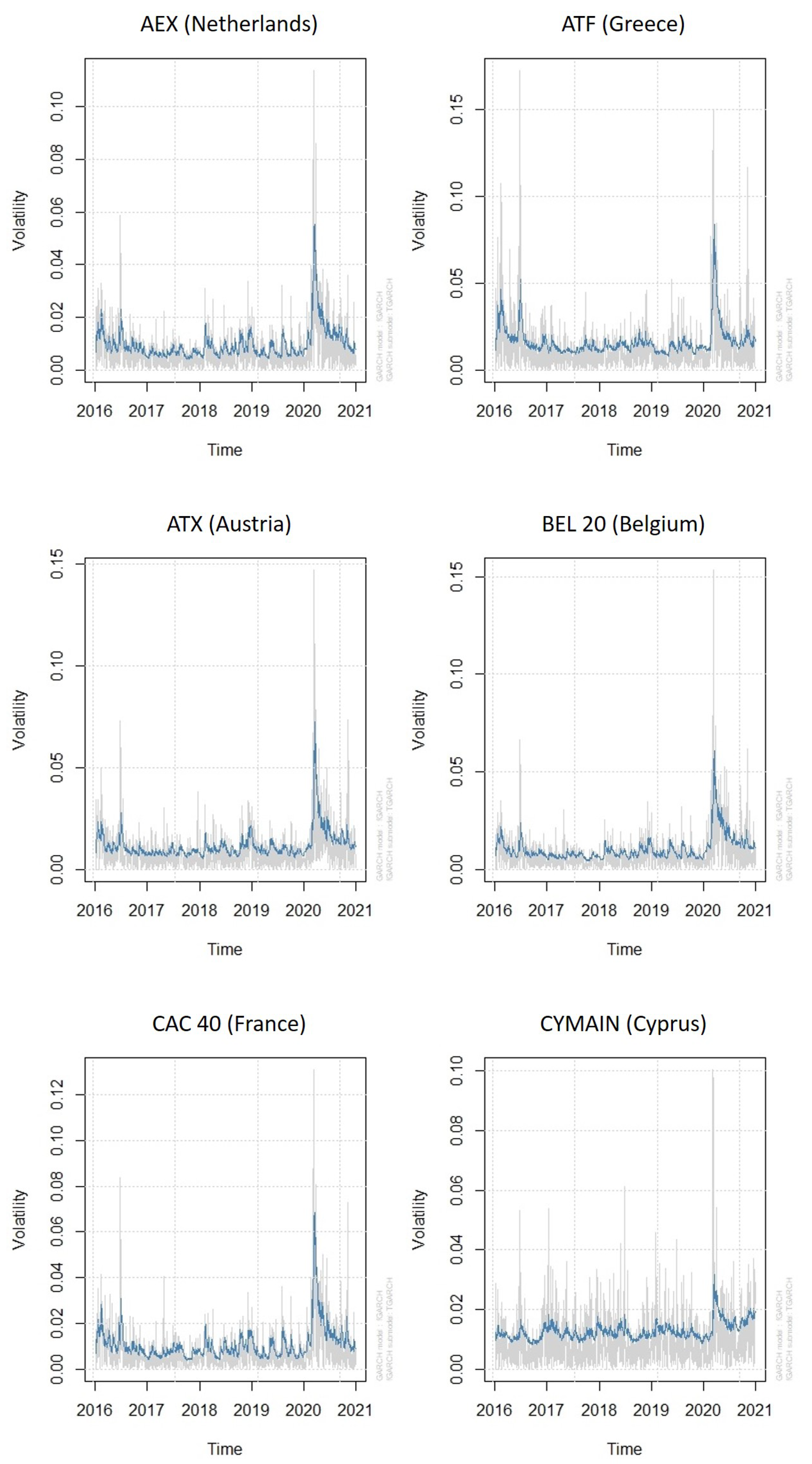
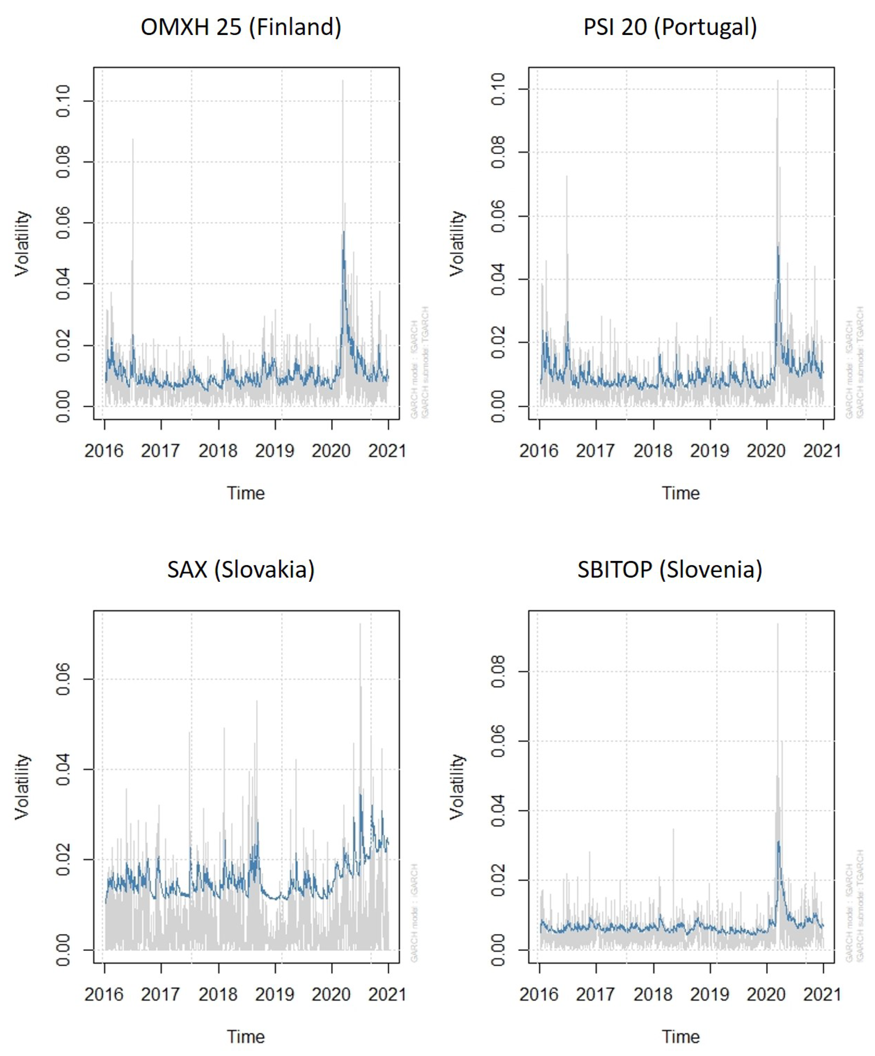
Appendix B. Conditional Volatility Plots

Figure A1. Estimated conditional standard deviation (volatility) versus absolute daily returns of euro area stock indices. Period from 4 January 2016 to 31 December 2020.
Mathematics 09 01212 g0a1
Figure A2. Estimated conditional standard deviation (volatility) versus absolute daily returns of euro area stock indices. Period from 4 January 2016 to 31 December 2020.
Mathematics 09 01212 g0a2
Figure A3. Estimated conditional standard deviation (volatility) versus absolute daily returns of euro area stock indices. Period from 4 January 2016 to 31 December 2020.
Mathematics 09 01212 g0a3

References

  1. Bhowmik, R.; Wang, S. Stock Market Volatility and Return Analysis: A Systematic Literature Review. Entropy 2020, 22, 522. [Google Scholar] [CrossRef]
  2. Jin, X.; An, X. Global financial crisis and emerging stock market contagion: A volatility impulse response function approach. Res. Int. Bus. Financ. 2016, 36, 179–195. [Google Scholar] [CrossRef]
  3. Neaime, S. Financial crises and contagion vulnerability of MENA stock markets. Emerg. Mark. Rev. 2016, 27, 14–35. [Google Scholar] [CrossRef]
  4. European Council. Timeline—Council Actions on COVID-19. Available online: https://www.consilium.europa.eu/en/policies/coronavirus/timeline/ (accessed on 17 February 2021).
  5. World Health Organization. Timeline: WHO’s COVID-19 Response. Available online: https://www.who.int/emergencies/diseases/novel-coronavirus-2019/interactive-timeline (accessed on 17 February 2021).
  6. Organisation for Economic Co-Operation and Development (OECD). OECD.Stat—Quarterly National Accounts: Quarterly Growth Rates of Real GDP, Change Over Previous Quarter. Available online: https://stats.oecd.org/index.aspx?queryid=350# (accessed on 19 February 2021).
  7. International Monetary Fund (IMF). World Economic Outlook Update (January 2020). Available online: https://www.imf.org/en/Publications/WEO/Issues/2021/01/26/2021-world-economic-outlook-update (accessed on 20 February 2021).
  8. Chaudhary, R.; Bakhshi, P.; Gupta, H. Volatility in International Stock Markets: An Empirical Study during COVID-19. J. Risk Financ. Manag. 2020, 13, 208. [Google Scholar] [CrossRef]
  9. Organisation for Economic Co-Operation and Development (OECD). GlobalFinancialMarketsPolicy Responses to COVID-19 (March 2020). Available online: https://www.oecd.org/coronavirus/policy-responses/global-financial-markets-policy-responses-to-covid-19-2d98c7e0/ (accessed on 19 February 2021).
  10. Cboe Global Markets. What is the VIX Index? Available online: https://www.cboe.com/tradable_products/vix/ (accessed on 20 February 2021).
  11. Cboe Global Markets. VIX Index Historical Data, VIX Data for 2004 to Present (Updated Daily). Available online: https://ww2.cboe.com/products/vix-index-volatility/vix-options-and-futures/vix-index/vix-historical-data# (accessed on 20 February 2021).
  12. Just, M.; Echaust, K. Stock market returns, volatility, correlation and liquidity during the COVID-19 crisis: Evidence from the Markov switching approach. Financ. Res. Lett. 2020, 37, 101775. [Google Scholar] [CrossRef] [PubMed]
  13. Baek, S.; Mohanty, S.K.; Glambosky, M. COVID-19 and stock market volatility: An industry level analysis. Financ. Res. Lett. 2020, 37, 101748. [Google Scholar] [CrossRef] [PubMed]
  14. Di Persio, L.; Garbelli, M.; Wallbaum, K. Forward-Looking Volatility Estimation for Risk-Managed Investment Strategies during the COVID-19 Crisis. Risks 2021, 9, 33. [Google Scholar] [CrossRef]
  15. Goswami, S.; Gupta, R.; Wohar, M.E. Historical volatility of advanced equity markets: The role of local and global crises. Financ. Res. Lett. 2020, 34, 101265. [Google Scholar] [CrossRef]
  16. Singhania, M.; Anchalia, J. Volatility in Asian stock markets and global financial crisis. J. Adv. Manag. Res. 2013, 10, 333–351. [Google Scholar] [CrossRef]
  17. Wasiuzzaman, S.; Angabini, A. GARCH Models and the Financial Crisis—A Study of the Malaysian Stock Market. Int. J. Appl. Econ. Financ. 2011, 5, 226–236. [Google Scholar] [CrossRef]
  18. Okičić, J. An Empirical Analysis of Stock Returns and Volatility: The Case of Stock Markets From Central And Eastern Europe. South East Eur. J. Econ. Bus. 2015, 9, 7–15. [Google Scholar] [CrossRef] [Green Version]
  19. Ahmad, W.; Bhanumurthy, N.; Sehgal, S. The Eurozone crisis and its contagion effects on the European stock markets. Stud. Econ. Financ. 2014, 31, 325–352. [Google Scholar] [CrossRef]
  20. Zhu, Z.; Bai, Z.; Vieito, J.P.; Wong, W.K. The impact of the global financial crisis on the efficiency and performance of Latin American stock markets. Estud. Econ. 2019, 46, 5–30. [Google Scholar] [CrossRef] [Green Version]
  21. Liu, H.; Manzoor, A.; Wang, C.; Zhang, L.; Manzoor, Z. The COVID-19 Outbreak and Affected Countries Stock Markets Response. Int. J. Environ. Res. Public Health 2020, 17, 2800. [Google Scholar] [CrossRef] [PubMed] [Green Version]
  22. Zaremba, A.; Kizys, R.; Aharon, D.Y.; Demir, E. Infected Markets: Novel Coronavirus, Government Interventions, and Stock Return Volatility around the Globe. Financ. Res. Lett. 2020, 35, 101597. [Google Scholar] [CrossRef]
  23. Engelhardt, N.; Krause, M.; Neukirchen, D.; Posch, P.N. Trust and stock market volatility during the COVID-19 crisis. Financ. Res. Lett. 2021, 38, 101873. [Google Scholar] [CrossRef]
  24. Yousef, I. Spillover of COVID-19: Impact on Stock Market Volatility. Int. J. Psychosoc. Rehabil. 2020, 24, PR261476. [Google Scholar] [CrossRef]
  25. Adenomon, M.O.; Maijamaa, B.; John, D.O. On the Effects of COVID-19 outbreak on the Nigerian Stock Exchange performance: Evidence from GARCH Models. Preprints 2020, 2020040444. [Google Scholar] [CrossRef] [Green Version]
  26. Shehzad, K.; Xiaoxing, L.; Kazouz, H. COVID-19’s disasters are perilous than Global Financial Crisis: A rumor or fact? Financ. Res. Lett. 2020, 36, 101669. [Google Scholar] [CrossRef]
  27. Szczygielski, J.J.; Bwanya, P.R.; Charteris, A.; Brzeszczynski, J. The only certainty is uncertainty: An analysis of the impact of COVID-19 uncertainty on regional stock markets. Financ. Res. Lett. 2021, 101945. [Google Scholar] [CrossRef] [PubMed]
  28. Bora, D.; Basistha, D. The outbreak of COVID-19 pandemic and its impact on stock market volatility: Evidence from a worst-affected economy. J. Public Aff. 2021, e2623. [Google Scholar] [CrossRef]
  29. Bhunia, A.; Ganguly, S. An assessment of volatility and leverage effect before and during the period of Covid-19: A study of selected international stock markets. Int. J. Financ. Serv. Manag. 2020, 10, 113–127. [Google Scholar] [CrossRef]
  30. Benzid, L.; Chebbi, K. The Impact of COVID-19 on Exchange Rate Volatility: Evidence Through GARCH Model. SSRN 2020. [Google Scholar] [CrossRef]
  31. Yousef, I.; Shehadeh, E. The Impact of COVID-19 on Gold Price Volatility. Int. J. Econ. Bus. Adm. (IJEBA) 2020, 8, 353–364. [Google Scholar] [CrossRef]
  32. Investing.com. European Indices. Available online: https://it.investing.com/indices/european-indices (accessed on 16 January 2021).
  33. Jarque, C.M.; Bera, A.K. Efficient tests for normality, homoscedasticity and serial independence of regression residuals. Econ. Lett. 1980, 6, 255–259. [Google Scholar] [CrossRef]
  34. Dickey, D.A.; Fuller, W.A. Distribution of the Estimators for Autoregressive Time Series with a Unit Root. J. Am. Stat. Assoc. 1979, 74, 427–431. [Google Scholar] [CrossRef]
  35. Phillips, P.C.B.; Perron, P. Testing for a unit root in time series regression. Biometrika 1988, 75, 335–346. [Google Scholar] [CrossRef]
  36. Box, G.E.P.; Pierce, D.A. Distribution of Residual Autocorrelations in Autoregressive-Integrated Moving Average Time Series Models. J. Am. Stat. Assoc. 1970, 65, 1509–1526. [Google Scholar] [CrossRef]
  37. Engle, R.F. Autoregressive Conditional Heteroscedasticity with Estimates of the Variance of United Kingdom Inflation. Econometrica 1982, 50, 987–1007. [Google Scholar] [CrossRef]
  38. Bollerslev, T. Generalized autoregressive conditional heteroskedasticity. J. Econom. 1986, 31, 307–327. [Google Scholar] [CrossRef] [Green Version]
  39. Mandelbrot, B. The Variation of Certain Speculative Prices. J. Bus. 1963, 36, 394–419. [Google Scholar] [CrossRef]
  40. Engle, R.F.; Lilien, D.M.; Robins, R.P. Estimating Time Varying Risk Premia in the Term Structure: The Arch-M Model. Econometrica 1987, 55, 391–407. [Google Scholar] [CrossRef]
  41. Francq, C.; Zakoian, J.M. GARCH Models: Structure, Statistical Inference and Financial Applications, 2nd ed.; John Wiley & Sons Ltd.: Hoboken, NJ, USA, 2019. [Google Scholar]
  42. Hentschel, L. All in the family Nesting symmetric and asymmetric GARCH models. J. Financ. Econ. 1995, 39, 71–104. [Google Scholar] [CrossRef]
  43. Zakoian, J.M. Threshold heteroskedastic models. J. Econ. Dyn. Control 1994, 18, 931–955. [Google Scholar] [CrossRef]
  44. Choudhry, T. Day of the week effect in emerging Asian stock markets: Evidence from the GARCH model. Appl. Financ. Econ. 2000, 10, 235–242. [Google Scholar] [CrossRef]
  45. Kiymaz, H.; Berument, H. The day of the week effect on stock market volatility and volume: International evidence. Rev. Financ. Econ. 2003, 12, 363–380. [Google Scholar] [CrossRef] [Green Version]
  46. Panait, I.; SlĂvescu, E.O. Using Garch-in-Mean Model to Investigate Volatility and Persistence at Different Frequencies for Bucharest Stock Exchange during 1997–2012. Theor. Appl. Econ. 2012, 19, 55–76. [Google Scholar]
  47. Ghalanos, A.; Kley, T. rugarch: Univariate GARCH Models. 2020. Available online: https://cran.r-project.org/web/packages/rugarch/index.html (accessed on 16 January 2021).
  48. Ghalanos, A. Introduction to the Rugarch Package. (Version 1.4-3). 2020. Available online: https://cran.r-project.org/web/packages/rugarch/vignettes/Introduction_to_the_rugarch_package.pdf (accessed on 16 January 2021).
  49. Fisher, T.J.; Gallagher, C.M. New Weighted Portmanteau Statistics for Time Series Goodness of Fit Testing. J. Am. Stat. Assoc. 2012, 107, 777–787. [Google Scholar] [CrossRef]
  50. Oxera Consulting LLP, European Commission. Primary and Secondary Equity Markets in the EU, Final Report, November 2020. Available online: https://www.oxera.com/publications/primary-and-secondary-equity-markets-in-the-eu/ (accessed on 2 February 2021).
  51. Engle, R.F.; Ghysels, E.; Sohn, B. Stock Market Volatility and Macroeconomic Fundamentals. Rev. Econ. Stat. 2013, 95, 776–797. [Google Scholar] [CrossRef]
  52. Conrad, C.; Custovic, A.; Ghysels, E. Long- and Short-Term Cryptocurrency Volatility Components: A GARCH-MIDAS Analysis. J. Risk Financ. Manag. 2018, 11, 23. [Google Scholar] [CrossRef]
  53. Salisu, A.A.; Gupta, R. Oil shocks and stock market volatility of the BRICS: A GARCH-MIDAS approach. Glob. Financ. J. 2021, 48, 100546. [Google Scholar] [CrossRef]
  54. Yu, X.; Huang, Y. The impact of economic policy uncertainty on stock volatility: Evidence from GARCH-MIDAS approach. Phys. A Stat. Mech. Its Appl. 2021, 570, 125794. [Google Scholar] [CrossRef]
Figure 1. Growth Rates of Gross Domestic Product compared to the same quarter of previous year, seasonally adjusted data (1st quarter 2016–4th quarter 2020).
Mathematics 09 01212 g001
Figure 2. Time plot of daily closing prices (4 January 2016–31 December 2020). Panel (a) contains the daily closing prices of Euro Stoxx 50 (STOXX50E). Panel (b) contains the daily closing prices of S&P 500 (SPX).
Mathematics 09 01212 g002
Figure 3. Estimated time-varying risk premium for the entire study period (4 January 2016–31 December 2020).
Mathematics 09 01212 g003
Figure 4. Relationship between real GDP per capita (Euro) and stock market capitalisation to GDP (%), 2018. Grey points represent small financial centers, while yellow points represent middle-large financial centers.
Mathematics 09 01212 g004
Table 1. Results of Conditional Volatility Equation.
IndicesEstimated Coefficients
ω vx 1 vx 2 α 1 γ 1 β 1 SkewShape
AEX0.0004 ***0.0004 **0.00010.0873 ***1.0000 ***0.8875 ***0.8192 ***7.2964 ***
ATF0.0006 ***0.00020.00020.1038 ***0.5067 ***0.8810 ***0.9046 ***4.9754 ***
ATX0.0005 ***0.0004 *0.00020.0801 ***1.0000 ***0.8840 ***0.8849 ***9.1205 ***
BEL 200.0004 ***0.0005 **0.0003 *0.0791 ***1.0000 ***0.8910 ***0.8614 ***6.3989 ***
CAC 400.0004 ***0.0005 *0.00020.1032 ***1.0000 ***0.8793 ***0.8709 ***5.6029 ***
CYMAIN0.0007 *0.00010.00030.1083 ***0.09460.3173 ***1.0090 ***5.3504 ***
DAX0.0004 ***0.0005 **0.00010.0850 ***1.0000 ***0.8916 ***0.8754 ***5.1223 ***
FTSE MIB0.0006 **0.0005 *0.00010.0878 ***1.0000 ***0.8789 ***0.8667 ***5.9696 ***
IBEX 350.0006 **0.0006 *0.00030.0940 ***0.7096 ***0.8679 ***0.8994 ***5.8759 ***
ISEQ 200.0004 ***0.0004 **0.0002 .0.0669 ***0.8617 ***0.9027 ***0.9281 ***7.3227 ***
MSE0.0010 **0.0005 .0.0006 .0.1863 ***0.3021 *0.6654 ***0.9168 ***3.7888 ***
OMXBBPI0.0003 **0.00020.00010.1373 ***0.11960.8420 ***0.9254 ***4.2957 ***
OMXH 250.0005 ***0.0004 **0.00010.0816 ***1.0000 ***0.8781 ***0.8589 ***10.6766 ***
PSI 200.0006 ***0.0003 .0.00030.1103 ***0.6996 ***0.8419 ***0.9172 ***7.2217 ***
SAX0.00000.00000.00000.1643 *0.06500.8357 *1.0157 ***2.1865 ***
SBITOP0.0003 **0.00020.00010.0878 ***0.3042 *0.8800 ***0.9752 ***5.2810 ***
Note:p-value significance codes 0 ‘***’ 0.001 ‘**’ 0.01 ‘*’ 0.05 ‘.’ 0.1 ‘ ’ 1. The CYMAIN model also includes the coefficient β 2 = 0.5420 ***.
Table 2. Estimated volatility peaks and volatility persistence.
IndicesVolatility Peaks Volatility Persistence
AEX0.0551 0.9540
ATF0.0840 0.9573
ATX0.0725 0.9458
BEL 200.0606 0.9507
CAC 400.0687 0.9562
CYMAIN0.0317 0.9395
DAX0.0626 0.9543
FTSE MIB0.0757 0.9447
IBEX 350.0621 0.9383
ISEQ 200.0505 0.9536
MSE0.0250 0.7954
OMXBBPI0.0415 0.9406
OMXH 250.0571 0.9415
PSI 200.0502 0.9258
SAX0.0345 1
SBITOP0.0313 0.9449
Publisher’s Note: MDPI stays neutral with regard to jurisdictional claims in published maps and institutional affiliations.

