Industrial Steel Heat Treating: Numerical Simulation of Induction Heating and Aquaquenching Cooling with Mechanical Effects

Abstract

This paper summarizes a mathematical model for the industrial heating and cooling processes of a steel workpiece corresponding to the steering rack of an automobile. The general purpose of the heat treatment process is to create the necessary hardness on critical parts of the workpiece. Hardening consists of heating the workpiece up to a threshold temperature followed by a rapid cooling such as aquaquenching. The high hardness is due to the steel phase transformation accompanying the rapid cooling resulting in non-equilibrium phases, one of which is the hard microconstituent of steel, namely martensite. The mathematical model describes both processes, heating and cooling. During the first one, heat is produced by Joule’s effect from a very high alternating current passing through the rack. This situation is governed by a set of coupled PDEs/ODEs involving the electric potential, the magnetic vector potential, the temperature, the austenite transformation, the stresses and the displacement field. Once the workpiece has reached the desired temperature, the current is switched off an the cooling stage starts by aquaquenching. In this case, the governing equations involve the temperature, the austenite and martensite phase fractions, the stresses and the displacement field. This mathematical model has been solved by the FEM and 2D numerical simulations are discussed along the paper.

1. Introduction and Description of the Industrial Procedure

This work deals with the thermomechanical modeling and the numerical simulation of metallurgical phase transitions of steel during an industrial heat treating.

Iron and steel production has a very long history that probably dates back to some millennia. For instance, Asian swords are legendary. They are straight and had double edged blades. The popularity of these swords can be explained by their extreme hardness, obtained through a traditional heating-cooling process. Hardness implies an increasing of brittleness, so that not both blade edges are hardened but only one of them, leaving the other one resistant to breakage.

Presently, steel represents a very important source of innovation. In fact, its toughness, good versatility and excellent processing properties make it one of the most commonly used in Engineering or as a building material.

Steel is an iron-based alloy containing small amounts of carbon and possibly some other elements. In the automotive industry, carbon content in steel lies between $0.2$ wt% and $2.1$ wt% and, together with other elements, represents the fundamental hardening agent, very useful to prevent dislocation motion and propagation, therefore increasing mechanical strength. It is possible to control the hardness, ductility and tensile strength of steel by changing the amount of carbon and other alloying elements, such a chromium, manganese, molybdenum, or vanadium.

Hardening consists of heating up the specified region till the austenitization is reached, followed by a very rapid cooling via aquaquenching, oil spraying or salt baths.

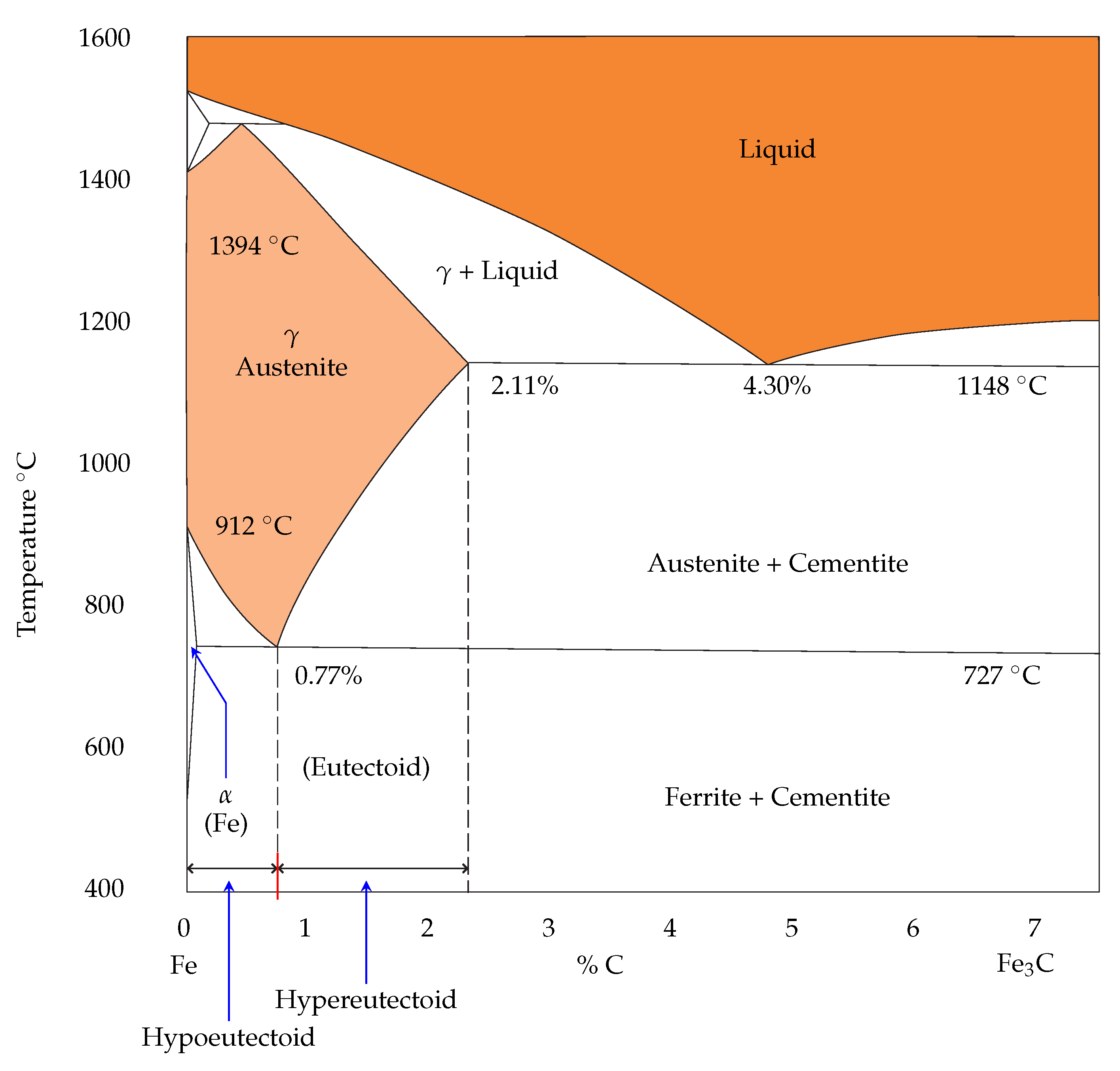
At room temperature, steel is composed by different solid phases: ferrite, pearlite, bainite, and martensite. In steels with less than $0.8$ wt% carbon, known as hypoeutectoid steel, it is possible to observe a significant variation of its internal structure in a temperature range between $727{}^{\circ }$C and $912{}^{\circ }$C, approximately. In this situation, all phases are transformed into austenite (or $\gamma -$iron). Figure 1 summarizes an iron-carbide phase diagram for carbon steel; it shows the condition under which the phases are stable.

When the cooling rate is high enough, the austenite is transformed into martensite, which is the hardest microconstituent of steel. On the other hand, if the cooling rate is not big enough, the austenite is transformed back into the other phases, i.e., ferrite, pearlite, and bainite (Figure 2) possibly along with a different partition.

There are some common situations in which the industrial requirement is such that the outer surface should be hard whereas the inner core should be kept ductile. In fact, this ensures the workpiece wear resistance while reducing at the same time the material fatigue.

There exist several industrial hardening procedure of steel: induction-conduction, flame, electron beam, laser surface, and so on (see [1,2,3]). For our purposes, we are concerned with an induction-conduction process. A conductor (coil) carries a high frequency alternating current producing a changing magnetic field and in its turn inducing eddy currents. As a result, induction heating takes place: the heat so generated (Joule’s heating) affects only the outer surface of steel components due to the skin effect. The current passing the workpiece is switched on usually for a few seconds only. When austenitization is reached, the electric current is then switched off and the workpiece is subsequently quenched in order to obtain the necessary cooling down temperature rate.

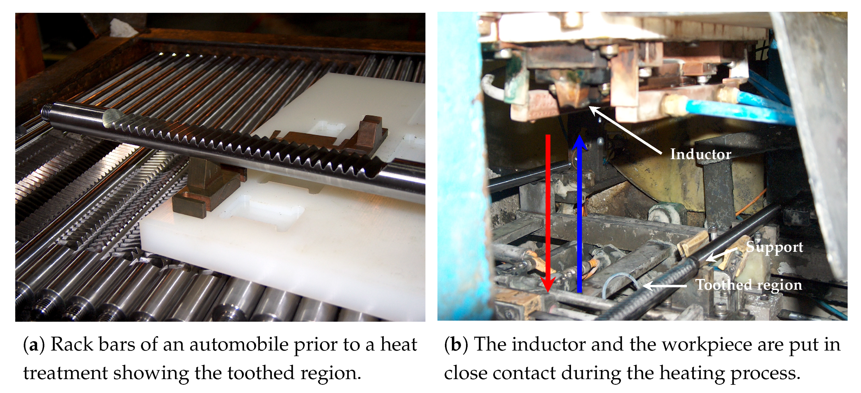
In this work we are interested in the mathematical description and the numerical simulation of the hardening procedure of a car steering rack (see Figure 3a) including mechanical effects. This mathematical description corresponds to the actual industrial procedure happening in situ at the manufacturer factory. The rack bar of an automobile is a cylindrical shape workpiece made of steel, provided with a toothed region designed to engage with a pinion: the rack bar is mounted in a pinion housing in order to be displaceable along the rack longitudinal axis. The rack bar is approximately 50 cm long and 22–25 mm in diameter. These two components, rack-pinion, constitute a very important part of the steering system of a vehicle: the manufacturer company must guarantee its correct performance for at least 20 years. The toothed region of the rack bar is permanently in close contact with the pinion, and along this contact surface strong stresses will appear. Thus, in order to avoid the mechanical deformations, hindering wear, abrasions and fractures, the toothed region has to be hardened but without changing the ductility within the rest of the workpiece.

In this paper, we will focus on the mathematical formulation of the phase transitions and the thermo-mechanical behavior of the workpiece. As long as the mechanical model is concerned, the main quantities of interest are (Cauchy) stress and strain tensors during the treatment and the displacement field. We assume that the strain may be additively decomposed into an elastic, a thermal, and a plastic part and that the thermomechanical problem is governed by the quasistatic momentum balance and the balance law of internal energy [4,5].

In the next section we describe the mathematical modeling of both the heating and the cooling industrial processes for the hardening of a rack bar. The governing equations is a nonlinear strongly coupled system of PDEs/ODEs. Figure 4 explains the way this whole system is strongly coupled concerning the electromagnetic quantities, the phase fractions, stresses, displacement field and temperature as well. Since a high alternating electric current (83 KHz in this setting) is applied, potential Maxwell’s equations in the harmonic regime are used to describe the electromagnetic induction. The main production term responsible for the increase in temperature along the critical part of the workpiece (the toothed region) is Joule’s heating coming from the eddy currents induced by the applied high alternating electric current. Additionally, we focus our attention on two solid steel phase fractions, namely austenite during the heating and cooling stages, and martensite during the cooling stage. The dynamics of these two phase fractions are described by a set of two ODEs. High temperature changes and phase transformations are accompanied by deformations. In order to deal with these mechanical effects, a quasistatic viscoelasticity model is considered. Here, the main quantities of interest are the Cauchy stress tensor, the strain tensor and the displacement field. Finally, a balance law of internal energy is taken into account. The source terms include Joule’s heating, mechanical dissipation and latent heat.

In Section 3 we present the numerical simulations of the model described in the previous section and comment the numerical results. All these numerical simulations have been carried out through the software package FreeFem++ [6]. This is a free programming language based on the finite element method. FreeFem++ is implemented in terms of the variational forms of the corresponding problems, so that it is straightforward to solve problems involving PDEs (both 2D or 3D) from several branches of physics and engineering.

Though the numerical simulations presented in this paper are in 2D, they may provide with a valuable information to the manufacturer company so that it may be useful to optimize this industrial process.

2. Mathematical Modeling

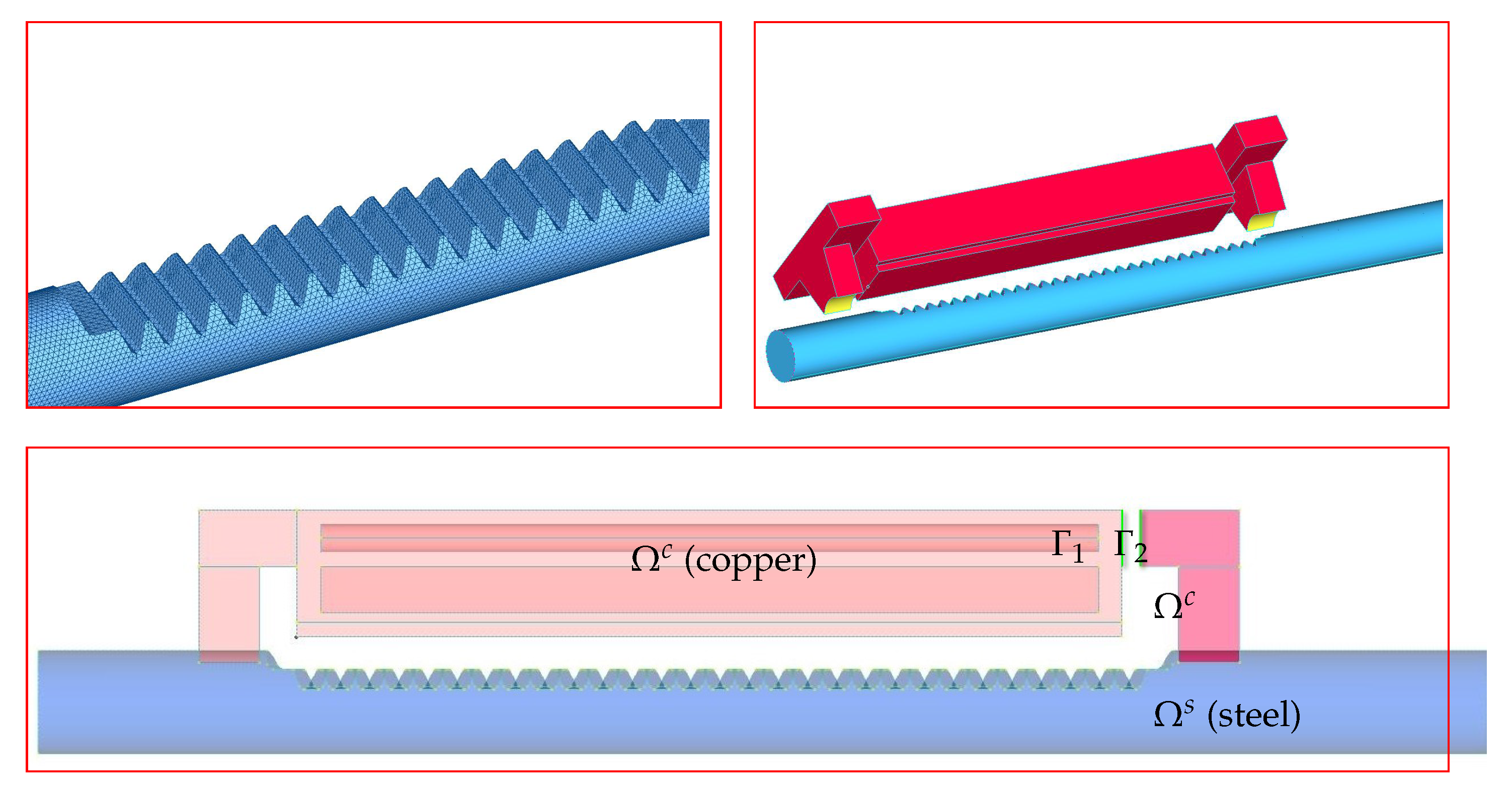
Let $\Omega \subset {\mathbb{R}}^N$$N=2,3$, be an open set with a Lipschitz-continuous boundary (see Figure 5). $\Omega ={\Omega }^{\mathrm{c}}\cup {\Omega }^{\mathrm{s}}\cup {\Gamma }^{\mathrm{ed}}$. ${\Omega }^{\mathrm{c}}$ and ${\Omega }^{\mathrm{s}}$ stand for the inductor (copper-made) and the steel rack bar, respectively. ${\Gamma }^{\mathrm{ed}}={\overline{\Omega }}^{\mathrm{c}}\cap {\overline{\Omega }}^{\mathrm{s}}$ is the contact surface between the two conductors. We consider two opposite faces ${\Gamma }_1,{\Gamma }_2\subset \partial {\Omega }^{\mathrm{c}}$ as shown in Figure 5 where the potential difference is applied. We also put $\Gamma ={\Gamma }_1\cup {\Gamma }_2$.

To deal with the heating-cooling stages, a time partition $[0,T_{\mathrm{f}}]=[0,T_{\mathrm{h}})\cup [T_{\mathrm{h}},T_{\mathrm{f}}]$, $T_{\mathrm{f}}>T_{\mathrm{h}}>0$ is considered. We distinguish our model in each time interval so that we may identify the main difficulties and phenomena involved. In both cases, the coupling between the thermomechanical phenomenon and the phase transformations will be analyzed [5,7,8,9,10,11].

The electromagnetic unknowns are $\phi$, standing for the scalar electric potential, and $\mathit{A}$ representing the complex magnetic field. The unknowns $\theta (x,t)$ and $u(x,t)$ stand for the temperature and the displacement field measured from the original geometry at the point $x\in {\Omega }^{\mathrm{s}}$ and at the instant $t\in [0,T_{\mathrm{f}}]$. By $a(x,t)$ (respectively, $m(x,t)$) we will denote the austenite (respectively, martensite) phase fraction. We consider an initial distribution of all steel phases given by $z_0$. This means that $z_0(x,t)+a(x,t)+m(x,t)=1$ for all $(x,t)\in {\overline{\Omega }}^{\mathrm{s}}\times [0,T_{\mathrm{f}}]$. Notice that, in this setting, we have $z_0(x,0)=1$ in ${\overline{\Omega }}^{\mathrm{s}}$.

2.1. Heating Stage: Governing Equations and Parameters Determination

The inductor and the rack bar are put in close contact as it is shown in Figure 5. In this setting, both conductors constitute the coil. During the time interval $(0,T_{\mathrm{h}})$ we let pass a high alternating current through the coil (83 KHz). The following equations will be considered [5,7,12,13,14]:

• Electromagnetics

$$\left\{\begin{array}{ccc}\hfill \nabla ·\left(b\right(\theta )\nabla \phi )& \hfill =& 0,\mathrm{in} {\Omega }_{T_{\mathrm{h}}}=\Omega \times (0,T_{\mathrm{h}}),\hfill \\ \hfill {\displaystyle \frac{\partial \phi }{\partial n}}& \hfill =& 0,\mathrm{on}(\partial \Omega \backslash \Gamma )\times (0,T_{\mathrm{h}}),\hfill \\ \hfill \phi =0 \mathrm{on} {\Gamma }_1\times (0,T_{\mathrm{h}}),& \hfill & \phi ={\phi }_0 \mathrm{on} {\Gamma }_2\times (0,T_{\mathrm{h}}),\hfill \\ \hfill b_0\left(\theta \right)i\omega \mathit{A}+\nabla \times \left(\frac{1}{\mu }\nabla \times \mathit{A}\right)& \hfill -& \delta \nabla (\nabla ·\mathit{A})=-b_0\left(\theta \right)\nabla \phi \mathrm{in}D\times (0,T_{\mathrm{h}}),\hfill \\ \hfill \mathit{A}& \hfill =& 0,\mathrm{on}\partial D\times (0,T_{\mathrm{h}}).\hfill \end{array}\right.$$

(1)

• Phase fractions

$$\left\{\begin{array}{ccccc}\hfill {\displaystyle \frac{\partial a}{\partial t}}& \hfill =& f_a(\theta ,a),\hfill & \mathrm{in}& {\Omega }^{\mathrm{s}}\times (0,T_{\mathrm{h}})\hfill \\ \hfill a\left(0\right)& \hfill =& 0,\hfill & \mathrm{in}& {\Omega }^{\mathrm{s}}.\hfill \end{array}\right.$$

(2)

• Deformations

$$\left\{\begin{array}{ccccc}\hfill \nabla ·\sigma \left(u\right)& \hfill =& \hfill 0,& \mathrm{in}& {\Omega }^{\mathrm{s}}\times (0,T_{\mathrm{h}}),\\ \hfill u& \hfill =& \hfill 0,& \mathrm{on}& {\Gamma }_{\mathrm{h}}^0\times (0,T_{\mathrm{h}}),\\ \hfill \sigma \left(u\right)·n& \hfill =& \hfill 0,& \mathrm{on}& {\Gamma }_{\mathrm{h}}^1\times (0,T_{\mathrm{h}}),\end{array}\right.$$

(3)

• with

$$\sigma \left(u\right)=K:\left(\epsilon \left(u\right)-q(\theta ,a)I\right).$$

(4)

• Temperature

$$\left\{\begin{array}{ccc}\hfill \alpha (\theta ,a,\sigma ){\displaystyle \frac{\partial \theta }{\partial t}}-\nabla ·(k\left(\theta \right)\nabla \theta )& \hfill =& \frac{1}{2}b\left(\theta \right){|i\omega \mathit{A}+\nabla \phi |}^2\hfill \\ & \hfill & +\beta (\theta ,a,\sigma ){\displaystyle \frac{\partial a}{\partial t}},\mathrm{in}{\Omega }^{\mathrm{s}}\times (0,T_{\mathrm{h}}),\hfill \\ \hfill \theta \left(0\right)& \hfill =& {\theta }_0,\mathrm{in}{\Omega }^{\mathrm{s}},\hfill \\ \hfill {\displaystyle \frac{\partial \theta }{\partial n}}& \hfill =& 0,\mathrm{on}\partial {\Omega }^{\mathrm{s}}\times (0,T_{\mathrm{h}}).\hfill \end{array}\right.$$

(5)

The system (1), describing the electromagnetic dynamics, comes from Maxwell’s equations in the harmonic regime. Here $b\left(\theta \right)$ is the electric conductivity, i is the imaginary unit, $\omega =2\pi \mathtt{f}$ is the pulsation, f being the frequency of the alternating current, $\mu =\mu \left(x\right)$ is the magnetic permeability, $\delta >0$ is a small constant and $b_0(x,s)=b(x,s)$ if $x\in \Omega$, $b_0(x,s)=0$ elsewhere;. Notice that $D\subset {\mathbb{R}}^2$ is a big enough and smooth domain containing the set of conductors. The magnetic permeability is then defined by the following piecewise constant function

$$\mu \left(x\right)=\left\{\begin{array}{cc}{\mu }_0\hfill & \mathrm{if}x\in D\backslash ({\Omega }^{\mathrm{c}}\cup {\Omega }^{\mathrm{s}}),\hfill \\ {\mu }_1\hfill & \mathrm{if}x\in {\Omega }^{\mathrm{s}},\hfill \\ {\mu }_2\hfill & \mathrm{if}x\in {\Omega }^{\mathrm{c}},\hfill \end{array}\right.$$

where the ${\mu }_0$, ${\mu }_1$ and ${\mu }_2$ stand for the vacuum permeability, steel permeability and copper permeability, respectively.

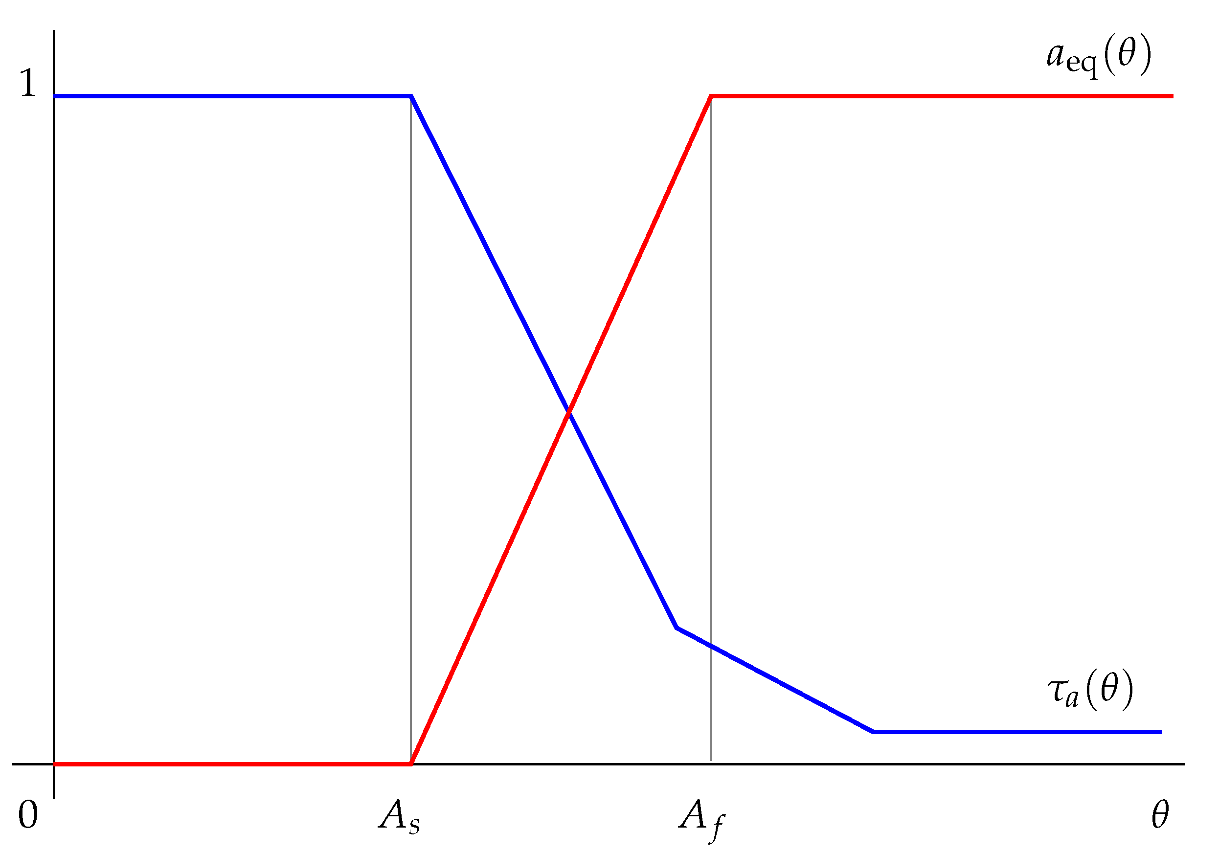
In Equation (2), a Leblond-Devaux model [15] is considered to simulate the austenite transformation once the threshold temperature $A_s$ is attained, particularly, the rate of change $f_a$ is modeled as

$$f_a(\theta ,a)=max\left\{\frac{1}{{\tau }_a\left(\theta \right)}(a_{\mathrm{eq}}\left(\theta \right)-a),0\right\}\mathcal{H}(\theta -A_s).$$

Herein, $\mathcal{H}$ stands for the Heaviside function $\mathcal{H}\left(s\right)=1$ if $s⩾0$ and is zero elsewhere. The functions $a_{\mathrm{eq}}\left(\theta \right)$, ${\tau }_a\left(\theta \right)$ (see Figure 6) can be determined from experimental data.

As far as the quasistatic model of viscoelasticity (3) is concerned, ${\Gamma }_{\mathrm{h}}^0\subset \partial {\Omega }^{\mathrm{s}}$ is the surface boundary where $\partial {\Omega }^{\mathrm{s}}$ is clamped (null displacement) during the heating stage and ${\Gamma }_{\mathrm{h}}^1=\partial {\Omega }^{\mathrm{s}}\backslash {\Gamma }_{\mathrm{h}}^0$. As it was said above, u is the displacement field and $\sigma$ denotes the stress tensor, related to strain $\epsilon \left(u\right)=\frac{1}{2}(\nabla u+\nabla u^{\mathrm{t}})$ through the constitutive law (4). In this last expression (see [16])

• K stands for the isotropic stiffness tensor;
• $q(\theta ,a)=q_0(1-a)(\theta -{\theta }_0^{\mathrm{ref}})+q_{a}a(\theta -{\theta }_a^{\mathrm{ref}})$ is a thermal contribution to strain, deduced from available dilatometry experiments (see Figure 7). As long as the temperature is increasing, the material expansion is modeled using a linear fitting. During the transformation into the austenite phase, a contraction range can be observed before going on with the usual expansion, but now with a higher linear coefficient.

Finally, arguing as in [5], a balance law is developed for the temperature. Thus, in (5), $k\left(\theta \right)$ stands for thermal conductivity, $\alpha$ and $\beta$ are given, respectively, by

$$\alpha (\theta ,a,\sigma )=\rho c+\mathrm{tr}\sigma \frac{\partial q}{\partial \theta },\beta (\theta ,a,\sigma )=\rho L+\mathrm{tr}\sigma \frac{\partial q}{\partial a},$$

$\rho$ being the steel density, c the specific heat at constant strain and L the latent heat. Additionally, ${\theta }_0$ is the room temperature, which is taken to be ${\theta }_0=300$ K in all our numerical experiments. The main production term in (5), responsible for the increasing in temperature is the quadratic term $\frac{1}{2}b\left(\theta \right){|i\omega \mathit{A}+\nabla \phi |}^2$ and is called Joule’s heating.

We put ${\theta }_{T_{\mathrm{h}}}=\theta \left(T_{\mathrm{h}}\right)$ and $a_{T_{\mathrm{h}}}=a\left(T_{\mathrm{h}}\right)$ the temperature distribution and the austenite fraction, respectively, at the end of the heating stage. Both functions ${\theta }_{T_{\mathrm{h}}}$ and $a_{T_{\mathrm{h}}}$ will be used as the initial temperature and austenite fraction, respectively, in the cooling stage.

2.2. Cooling Stage: Governing Equations and Parameters Determination

At $t=T_{\mathrm{h}}$ the current is switched off and for $T_{\mathrm{h}}⩽t⩽T_{\mathrm{f}}$, the aquaquenching takes place. The workpiece is sprayed down with oily water at a constant temperature ${\theta }_{\mathrm{q}}$. The temperature goes down so quickly in the austenized toothed region that the martensite phase fraction is forced to appear. However, these phase transformations induce a plastic deformation. According to [17,18], this TRIP (TRansformation-Induced-Plasticity) contribution to strain for the austenite-martensite transformation is taken into account in our model.

• Phase fractions

$$\left\{\begin{array}{cccc}\hfill {\displaystyle \frac{\partial a}{\partial t}}& \hfill =& f_a(\theta ,a)-{\displaystyle \frac{\partial m}{\partial t}},\hfill & \mathrm{in}{\Omega }^{\mathrm{s}}\times (T_{\mathrm{h}},T_{\mathrm{f}}),\hfill \\ \hfill {\displaystyle \frac{\partial m}{\partial t}}& \hfill =& f_m\left(a,m,\theta ,{\displaystyle \frac{\partial \theta }{\partial t}}\right),\hfill & \mathrm{in}{\Omega }^{\mathrm{s}}\times (T_{\mathrm{h}},T_{\mathrm{f}}),\hfill \\ \hfill a\left(T_{\mathrm{h}}\right)& \hfill =& a_{T_{\mathrm{h}}},\hfill & \mathrm{in}{\Omega }^{\mathrm{s}},\hfill \\ \hfill m\left(T_{\mathrm{h}}\right)& \hfill =& 0,\hfill & \mathrm{in}{\Omega }^{\mathrm{s}}.\hfill \end{array}\right.$$

(6)

• Deformations

$$\left\{\begin{array}{cccc}\hfill \nabla ·\sigma \left(u\right)& \hfill =& \hfill 0,& \mathrm{in}{\Omega }^{\mathrm{s}}\times (T_{\mathrm{h}},T_{\mathrm{f}}),\\ \hfill u& \hfill =& \hfill 0,& \mathrm{on}{\Gamma }_{\mathrm{c}}^0\times (T_{\mathrm{h}},T_{\mathrm{f}}),\\ \hfill \sigma \left(u\right)·n& \hfill =& \hfill 0,& \mathrm{on}{\Gamma }_{\mathrm{c}}^1\times (T_{\mathrm{h}},T_{\mathrm{f}}),\end{array}\right.$$

(7)

$$\sigma \left(u\right)=K:\left({\displaystyle \epsilon \left(u\right)-q(\theta ,a,m)I-{\int }_0^t\gamma \left(\theta ,m,{\displaystyle \frac{\partial m}{\partial t}}\right)S\mathrm{d}\tau }\right).$$

(8)

• Temperature

$$\left\{\begin{array}{ccc}\hfill \alpha (\theta ,a,m,\sigma ){\displaystyle \frac{\partial \theta }{\partial t}}& \hfill -& \nabla ·(k\left(\theta \right)\nabla \theta )={\beta }_a(\theta ,a,m,\sigma ){\displaystyle \frac{\partial a}{\partial t}}\hfill \\ \hfill & \hfill +& {\beta }_m(\theta ,a,m,\sigma ){\displaystyle \frac{\partial m}{\partial t}}+\gamma \left(\theta ,m,{\displaystyle \frac{\partial m}{\partial t}}\right){\left|S\right|}^2,\mathrm{in}{\Omega }^{\mathrm{s}}\times (T_{\mathrm{h}},T_{\mathrm{f}})\hfill \\ \hfill & \hfill & \theta \left(T_{\mathrm{h}}\right)={\theta }_{T_{\mathrm{h}}},\mathrm{in}{\Omega }^{\mathrm{s}},\hfill \\ \hfill & \hfill & -k\left(\theta \right){\displaystyle \frac{\partial \theta }{\partial n}}=\overline{\beta }(\theta -{\theta }_{\mathrm{q}}),\mathrm{on}\partial {\Omega }^{\mathrm{s}}\times (T_{\mathrm{h}},T_{\mathrm{f}}).\hfill \end{array}\right.$$

(9)

In (6), a Koistinen-Marburger model is taken into account in order to describe the martensite transformation (see [19]). This diffusionless transformation is quite different from that related to austenite and it is highly dependent on the cooling rate:

$$f_m\left(a,m,\theta ,{\displaystyle \frac{\partial \theta }{\partial t}}\right)=c_{m}a\mathcal{H}\left(-{\displaystyle \frac{\partial \theta }{\partial t}}\right)\mathcal{H}(M_s-\theta ),$$

where the threshold value $M_s$ indicates the starting temperature from which the martensite appears, whereas $c_m$ is a constant determined from experimental data.

In (7) and (8), the thermal strain should be conveniently modified in order to take into account the new linear growing during the cooling as is shown in Figure 7. This yields

$$q(\theta ,a,m)=q_0(1-a-m)\left(\theta -{\theta }_0^{\mathrm{ref}}\right)+q_{a}a\left(\theta -{\theta }_a^{\mathrm{ref}}\right)+q_{m}m\left(\theta -{\theta }_m^{\mathrm{ref}}\right).$$

Moreover, as in [7,20] the TRIP effect is modeled by

$$\frac{\partial {\epsilon }^{\mathrm{trip}}}{\partial t}={\lambda }_1\left(\theta \right)\frac{\partial {\lambda }_2\left(m\right)}{\partial m}\frac{\partial m}{\partial t}S\stackrel{\mathrm{def}}{=}\gamma \left(\theta ,m,\frac{\partial m}{\partial t}\right)S,$$

(10)

where $S=\sigma -\frac{1}{N}\left(\mathrm{tr}\sigma \right)I$ is the deviatoric stress tensor and $\mathrm{tr}\sigma$ denotes the trace of $\sigma$; ${\lambda }_1\left(\theta \right)=\frac{3}{2}\mathcal{K}$, and $\mathcal{K}$ is experimentally determined; ${\lambda }_2$ is a suitably selected increasing function such that ${\lambda }_2\left(0\right)=0$ and ${\lambda }_2\left(1\right)=1$, for instance ${\lambda }_2\left(s\right)=s(2-s)$ as in [17], or ${\lambda }_2\left(s\right)=s(1-log\left(s\right))$ as in [18].

Finally, in (9) the functions ${\beta }_a$ and ${\beta }_m$ are given by

$${\beta }_a(\theta ,a,m,\sigma )=-\rho L+\mathrm{tr}\sigma \frac{\partial q}{\partial a}\mathrm{and}{\beta }_m(\theta ,a,m,\sigma )=\rho L+\mathrm{tr}\sigma \frac{\partial q}{\partial m}.$$

Notice that the aquaquenching is modeled through the Robin boundary condition in (9) where $\overline{\beta }$ stands for a heat transfer coefficient.

3. Numerical Simulations

Using the FreeFem++ software [6] we carried out some numerical simulations of the model (1)–(9). We used the finite element method for the space approximation and a Crank-Nicolson scheme for the time discretization. Actually, a $P_2$-Lagrange approximation for $\phi$, $\mathit{A}$, $\theta$ and u, and $P_1$ for a and m. Ordinary differential equations are discretized using Heun’s method.

A fixed time step has been used from $t=0$ to $t=T_{\mathrm{h}}=5.5$, namely $\Delta t=5.5/110$, whereas a variable time step has been considered from $t=T_{\mathrm{h}}$ to $t=T_{\mathrm{f}}=11.0$ in order to deal with the drastic decreasing in temperature during the first iterations of the cooling stage. To do so, we first consider the function $s\left(t\right)={(t-5.5)}^2/5.5$ and put $r_0=t_0=5.5$, then define recursively for $n=1,\dots ,110$,

$$r_n=r_{n-1}+\Delta t \mathrm{and} t_n=t_{n-1}+s\left(r_n\right)-s\left(r_{n-1}\right).$$

In this way, the first time iterations of the cooling stage refer to tighter time steps than the ones of the final iterations.

In our simulation, the workpiece was heated up during $T_{\mathrm{h}}=5.5$ s from a room temperature of ${\theta }_0=300$ K followed by the aquaquenching for another $5.5$ s ($T_{\mathrm{f}}=11$). The temperature of the oil used in the aquaquenching is ${\theta }_{\mathrm{q}}=315$ K.

In Figure 8, some pictures are displayed for the meshes used in our 2D numerical simulations. It is important to have a high density of triangles close to the toothed region. The material parameters have been taken from data of a specific steel with a given composition (

Table 1. Chemical composition of 42CrMo4 steel.

Elements	C	Si	Mn	P	S	Cr	Cu	Mo	Ni
Content %wt	0.420	0.260	0.680	0.019	0.021	1.020	0.330	0.180	0.150

) assuring the desirable mechanical properties after the heat treating [21]. In

Table 2. Electromagnetic and metallurgical data.

Vacuum permeability	${\mathit{\mu }}_0$	$4\mathit{\pi }\times {10}^{-7}$	$\mathrm{N}/{\mathrm{A}}^2$
Steel permeability	${\mu }_1$	$2.24\times {10}^3$${\mu }_0$	$\mathrm{N}/{\mathrm{A}}^2$
Copper permeability	${\mu }_2$	0.99995${\mu }_0$	$\mathrm{N}/{\mathrm{A}}^2$
Current frequency	f	$8.3\times {10}^4$	$\mathrm{Hz}$
Pulsation	$\omega$	$2\pi \mathtt{f}$	$\mathrm{Hz}$
Density	$\rho$	7653.00	$\mathrm{Kg}/{\mathrm{m}}^3$
Specific heat	c	554.00	$\mathrm{J}/(\mathrm{Kg} \mathrm{K})$
Thermal conductivity	k	34.28	$\mathrm{J}/(\mathrm{s} \mathrm{m} \mathrm{K})$
Latent heat	L	$8.20\times {10}^4$	$\mathrm{J}/\mathrm{Kg}$
Young modulus	E	$21.00\times {10}^{10}$	$\mathrm{Pa}$
Poisson coefficient	$\nu$	0.28	-
Plasticity constant	$\mathcal{K}$	$4.20\times {10}^{-11}$	-
Austenite starting temperature	$A_s$	1003.00	$\mathrm{K}$
Austenite finishing temperature	$A_f$	1113.00	$\mathrm{K}$
Martensite starting temperature	$M_s$	633.00	$\mathrm{K}$
Steel thermal coefficient	$q_0$	$1.53\times {10}^{-5}$	${\mathrm{K}}^{-1}$
Reference temperature	${\theta }_{\mathrm{ref}}^0$	300.00	$\mathrm{K}$
Austenite thermal coefficient	$q_a$	$2.46\times {10}^{-5}$	${\mathrm{K}}^{-1}$
Reference temperature	${\theta }_{\mathrm{ref}}^a$	701.00	$\mathrm{K}$
Martensite thermal coefficient	$q_m$	$1.15\times {10}^{-5}$	${\mathrm{K}}^{-1}$
Reference temperature	${\theta }_{\mathrm{ref}}^m$	298.00	$\mathrm{K}$
Heat transfer coefficient	$\overline{\beta }$	$6.6\times {10}^3$	$\mathrm{W}/({\mathrm{m}}^2 \mathrm{K})$
Aquaquenching oil temperature	${\theta }_{\mathrm{q}}$	315.00	$\mathrm{K}$

we can find the actual values we have taken in our numerical experiments. The parameters in the thermal stresses modeling has been taken from [22,23].

Additionally, the value of the small parameter $\delta$ appearing in the equation for the complex magnetic field is taken to be $\delta ={10}^{-15}$. In fact, the term $-\delta \nabla (\nabla ·\mathit{A})$ appearing in (1) is artificial. It is used in order to stabilize the numerical resolution of (1). Of course, other approaches are possible (see [5,7]).

In [12,24], some theoretical and numerical results can be found for a simplified version of this problem, without taking into account mechanical effects. In [14] some additional details of the numerical Freefem++ code about the construction of the toothed geometry are described.

In Figure 9, the austenite profile is shown for some selected time instants during the heating stage, along with the temperature distribution at the same time instants. During the cooling stage, the austenite is fully transformed and the martensite is obtained as long as the temperature has decreased rapidly (Figure 10). The evolution of the phase fractions austenite and martensite and the temperature has been measured on three selected points A, B and C lying at different heights within one tooth. The evolution of these quantities are depicted in Figure 11. Due to the eddy currents and the skin effect along the toothed region, the temperature is higher on point A than on B, and on this one than on C. As a result, austenitization is reached first on point A, then on B and then on C. Notice the drastic decreased of the temperature at the beginning of the aquaquenching on these three points. Finally, the austenite is transformed into martensite but the amount of the computed martensite fraction is slightly higher on B and C than on point A.

As far as the mechanical deformations are concerned, Figure 12 and Figure 13 show the deformed meshes corresponding to the end of both the heating and the cooling stages. In both cases, they are compared to the original mesh. For $t\in [0,T_{\mathrm{h}})$, we assume that the rack bar is clamped at four boundary sites, namely up and down and at both sides of the toothed region. For $t\in [T_{\mathrm{h}},T_{\mathrm{f}}]$, the rack is released on the two upper boundaries, but it is still clamped on the two boundaries below. Since austenite is a face-centered cubic structure it is denser than the other phases. For this reason, during the heating stage all the austenized region will result in a volume reduction and in its turn a deformed configuration. This shrinking is put in evidence in Figure 12. On the other hand, during the cooling stage the transformation from austenite into martensite will produce a slight increase in volume which deforms the rack bar as shown in Figure 13. Obviously, just after this treatment, the rack bar needs to be rectified in order to recover its straightness at least at an admissible threshold. Obviously, due to these deformations the workpiece is highly stressed in some particular regions. 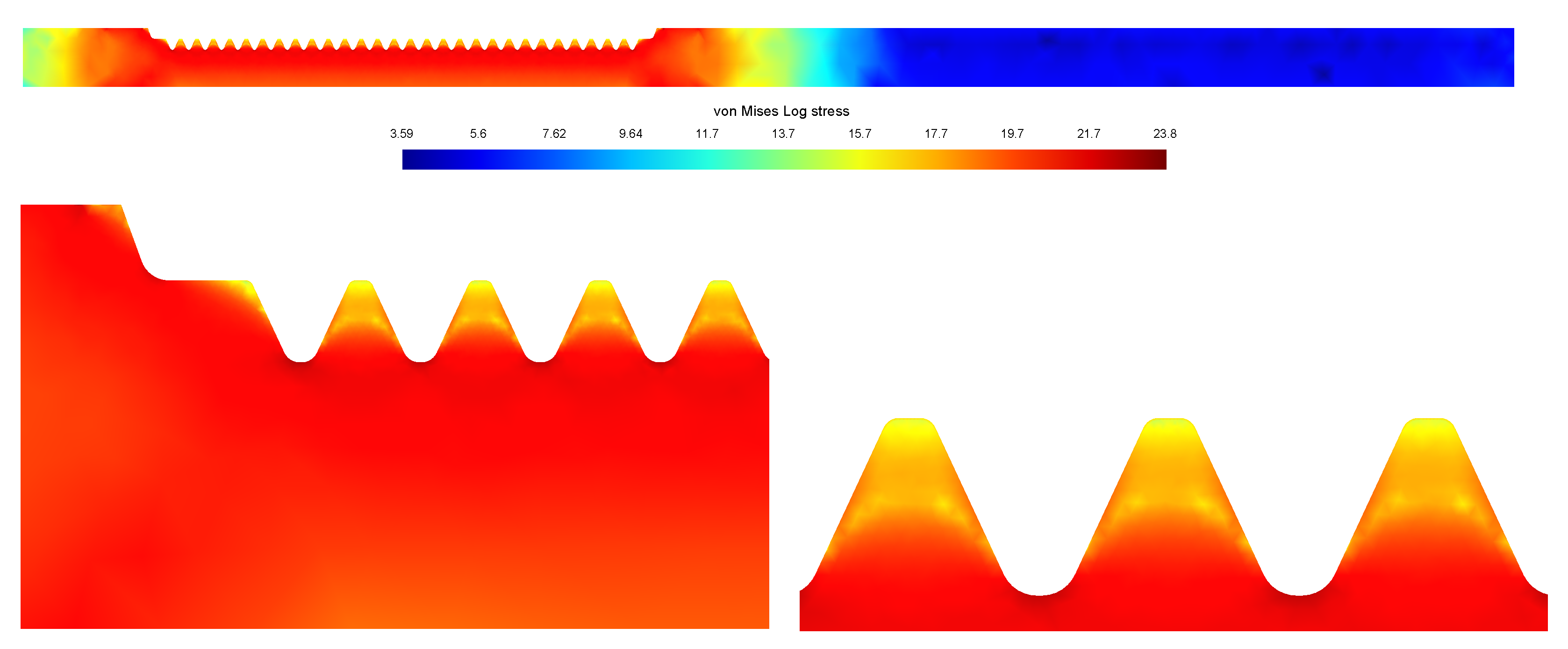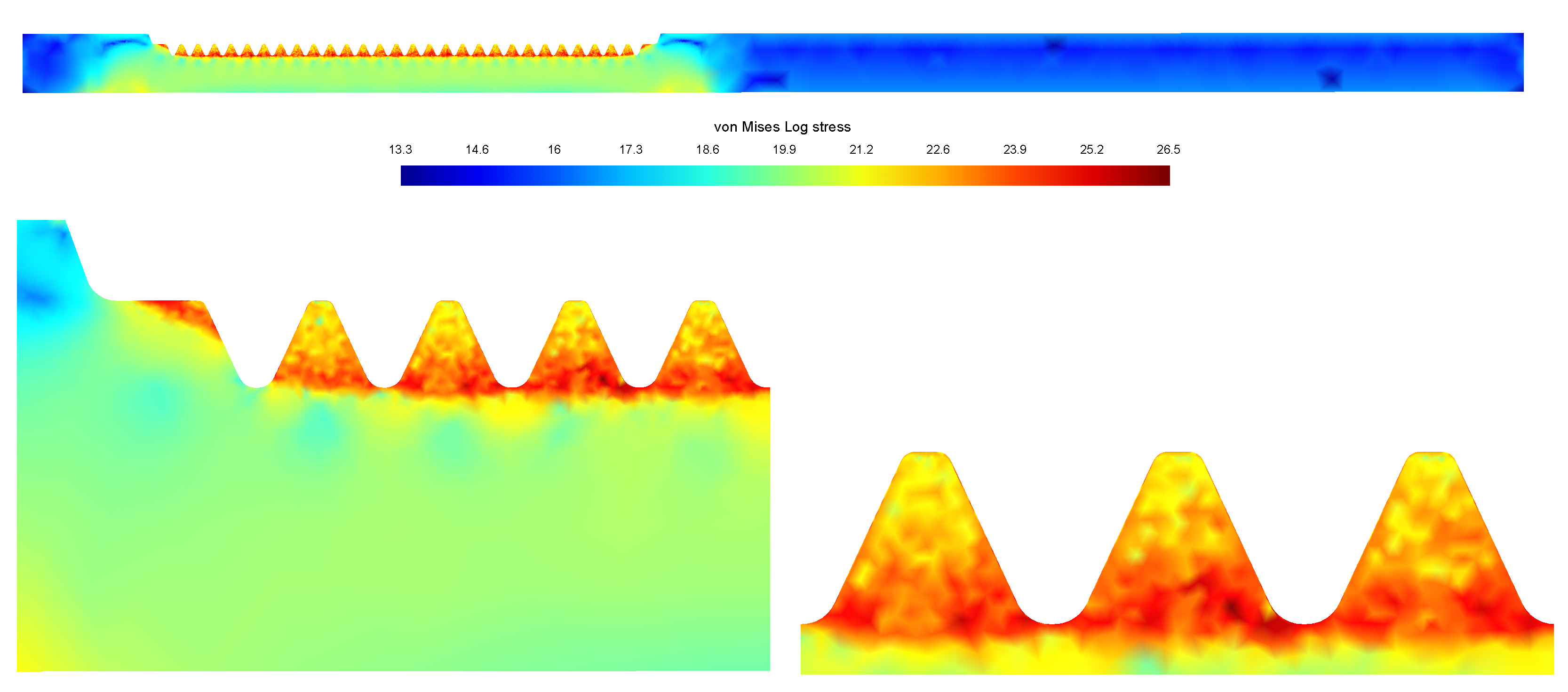Figure 14 and Figure 15 depicts the distribution of the (natural logarithm of) von Mises stresses at the end of the heating and cooling stages, respectively. At the end of the heating stage, according to Figure 14, the toothed line and the region below it is highly stressed. On the other hand, at the end of the cooling stage, the workpiece is extremely stressed along the toothed line whereas below it the workpiece undergoes some stress reduction, as shown in Figure 15. In both cases, almost the same stress pattern is found at each tooth. These residual stresses in the workpiece can be reduced by a heat treating called tempering. As a result, the hardness obtained after the quenching will decrease up to a level still suitable for the application.

4. Conclusions

This paper describes a problem related to the industrial heating-cooling process of a steel workpiece corresponding to the steering rack of an automobile. Precisely, the mathematical problem consists of a nonlinear system of ODEs for both steel phase fractions, austenite and martensite, coupled with a strongly coupled and nonlinear system of PDEs for the electric potential, the complex magnetic field, stresses and displacement field and the temperature.

Many industrial heating procedures are based on an AC induction technique so that the workpiece is put near the coil but with neat separation between them. However, this is not the case described in this paper, mainly due to the special geometry of the considered workpiece.

In this setting, the inductor machine and the workpiece are put in close contact so that all together constitute a coil. The eddy currents combined with the skin effect result in Joule’s heating along the toothed region of the rack bar which leads to the high heating of the workpiece critical part.

Once the mathematical model has been fully described, including all the relevant physical quantities, we carried out some numerical simulations based on the FEM. To do so, we have considered a mesh exhibiting an element high density around the rack toothed region.

Though we only performed 2D numerical simulations, all these numerical results may provide a valuable information to the manufacturer and can be useful in order to optimize this industrial process.

The analysis of the numerical simulations shows how the toothed region along the rack bar is heated up until austenitization is reached. During this stage, one can observe the mechanical effects on the workpiece: expansions due to the raise of temperature and at the same time volume reduction on the austenitized region. On the other hand, during the aquaquenching, the toothed region is radically cooled down so that martensite is produced along the toothed region and again some mechanical effects are observed: the workpiece undergoes expansions where martensite occurs and contractions elsewhere.

Moreover, the rate-dependent inelastic behavior of the workpiece is justified by the plastic term appearing in the constitutive laws. The austenite transformation induces the teeth shrinking during heating; successively, the same workpiece expands again during cooling according to the martensite transformation, but without reaching its initial configuration. Obviously, these deformations are accompanied by stresses. A computation of the von Mises stresses has shown the regions where the workpiece is particularly stressed.

The next step in this research should be to implement the resolution of this model in a 3D setting.