Numerical Solution of the Fredholm and Volterra Integral Equations by Using Modified Bernstein–Kantorovich Operators

Abstract

The main aim of this paper is to numerically solve the first kind linear Fredholm and Volterra integral equations by using Modified Bernstein–Kantorovich operators. The unknown function in the first kind integral equation is approximated by using the Modified Bernstein–Kantorovich operators. Hence, by using discretization, the obtained linear equations are transformed into systems of algebraic linear equations. Due to the sensitivity of the solutions on the input data, significant difficulties may be encountered, leading to instabilities in the results during actualization. Consequently, to improve on the stability of the solutions which imply the accuracy of the desired results, regularization features are built into the proposed numerical approach. More stable approximations to the solutions of the Fredholm and Volterra integral equations are obtained especially when high order approximations are used by the Modified Bernstein–Kantorovich operators. Test problems are constructed to show the computational efficiency, applicability and the accuracy of the method. Furthermore, the method is also applied to second kind Volterra integral equations.

1. Introduction

Fredholm and Volterra integral equations of the first kind play an important role in many problems from science and engineering. It is known that the Fredholm integral equations can be derived from boundary value problems with given boundary conditions. For example, Fredholm integral equations of the first kind arise in a mathematical model of the transport of fluorescein across the blood–retina barrier in the transient state and the subsequent diffusion of fluorescein in the vitreous body given in Larsen et al. [1]. Some other applications are in palaeoclimatology given in Anderssen and Saull [2], antenna design in Herrington [3], astrometry in Craig and Brown [4], image restoration in Andrews and Hunt [5]. The investigation of Volterra integral equations is very important in solving initial value problems of usual and fractional differential equations arising from the mathematical modelling of many scientific problems, including population dynamics, spread of epidemics, and semi-conductor devices, such as the biological fractional n-species delayed cooperation model of Lotka–Volterra type given in Tuladhar et al. [6]. Examples of Volterra integral equations of first kind can be extended to mathematical model of animal studies of the effect of the deposition of radioactive debris in the lung by Hendry [7], the heat conduction problem in Bartoshevich [8], tautochrone problem of which Abel’s integral equation was derived by Abel [9], (see also Groetsch [10]), electroelastic of dynamics of a nonhomogeneous spherically isotropic piezoelectric hollow sphere problem in Ding et al. [11]. Additionally, the use of a dynamical model of Volterra integral equations in energy storage with renewable and diesel generation has been analysed in Sidorov et al. [12].

As a classical ill-posed problem, the numerical solution of Fredholm integral equations of the first kind has been investigated by many authors, as a former study by Phillips [13] and a recent study by Neggal et al. [14]. The well-known early methods are the regularization methods given with a technique by Phillips in [13] and the Tikhonov regularization by Tikhonov in [15,16]. In the Tikhonov method, a continuous functional is usually used and the minimizer for the corresponding functional is difficult to obtain. Consequently, several methods have been proposed to obtain an effective choice of the regularization parameter in Tikhonov method such as the discrepancy principle, the quasi-optimality criterion (see Groetsch [17], Bazan [18] and references therein). Further, in Caldwell [19], a direct quadrature method and a boundary-integral method were examined for solving Fredholm integral equations of the first kind. Additionally, a regularization technique which replaces ill-posed equations of the first kind by well-posed equations of the second kind was employed to produce meaningful results for comparison purposes. Later, the extrapolation technique by Brezinski et al. [20] and a modified Tikhonov regularization method to solve the Fredholm integral equation of the first kind under the assumption that measured data are contaminated with deterministic errors was given in Wen and Wei [21]. Recently, a variant of projected Tikhonov regularization method for solving Fredholm integral equations of the first kind was proposed in Neggal et al. [14] in which for the subspace of projection, the Legendre polynomials were used.

Early studies for the solution of Volterra integral equations of the first kind involve the high order block by block methods in Hoog and Weiss [22,23]. However, these methods suffer from the disadvantage of requiring additional evaluations of the kernels and the solution of systems of algebraic equations for each step. Later, Taylor [24] used inverted differentiation formulae, which the resulting methods were explicit corresponding to local differentiation formulae. As the author stated “the main disadvantage of this method is that weights must be calculated from the recurrence relation (2.9) and the differentiation formula must be chosen so that the Dahlquist root condition is satisfied”. Integral equations of the first kind associated with strictly monotone Volterra integral operators were solved in Brunner [25] by projecting the exact solution of such an equation into the space $S_m^{(-1)}\left(Z_N\right)$ of piecewise polynomials of degree $m\ge 0$ possessing jump discontinuities on the set $Z_N$ of knots. Besides, the asymptotic behavior of solutions to nonlinear Volterra integral equations was analysed in Hulbert and Reich [26]. The future-sequential regularization method and predictor-corrector regularization method for the approximation of Volterra integral problems of first kind with convolution kernel were given in Lamm [27] and Lamm [28], respectively. The numerical solution of Volterra integral equations of the first kind by sequential Tikhonov regularization coupled with several standard discretizations (collocation-based methods, rectangular quadrature, or midpoint quadrature) was given in Lamm and Eldén [29].

New approaches have been developed for the solution of integral equations that use the basis functions and transform the integral equation to the system of linear or nonlinear equations. One of these approaches is the use of wavelet basis. For the solution of Abel’s integral equation, Legendre wavelets were used in Yousefi [30] and the wavelet basis were used in Maleknejad et al. [31] for the numerical solution of Volterra type integral equations of the first kind. Another approach is the use of polynomial approximations. In Mandal and Bhattacharya [32], Fredholm integral equations of the second kind and a simple hypersingular integral equation and a hypersingular integral equation of the second kind were numerically solved using Bernstein polynomials. At the same year, in Maleknejad et al. [33] numerical solution of linear and nonlinear Volterra integral equations, of the second kind by using Chebyshev polynomials was given. Afterwards, a new approach to the numerical solution of Volterra integral equations by using Bernstein’s approximation was given in Maleknejad et al. [34].

Recently, exhaustive studies on the use of CESTAC method for the solution of Volterra first type integral equations has been given in Noeiaghdam et al. [35] in which the control of accuracy on Taylor-collocation method to solve the weakly regular Volterra integral equations of the first kind has been studied. Furthermore, in Noeiaghdam et al. [36] that the numerical validation of the Adomian decomposition method for solving Volterra integral equation with discontinuous kernels was given.

The need of stable, reliable and time efficient methods for the numerical solution of Fredholm and Volterra integral equations of first kind is the main motivation of contributions. The achievements of the study can be summarised as follows:

1. Using the Modified Bernstein–Kantorovich operators, a numerical approach is developed for the solution of Fredholm and Volterra integral equations of the first kind with continuous and square integrable kernels. Convergence analysis are given assuming that minimum norm least square solution of the obtained algebraic linear systems are obtained by using the exact data, that is to say the Moore–Penrose inverse of the resulting coefficient matrices are computed exactly.

2. Furthermore, regularized integral equations are considered to obtain more smooth solutions especially when high-order approximations are used by Modified Bernstein–Kantorovich operators. The proposed approach is applied by building regularization features into the algorithm and perturbation error analysis are given.

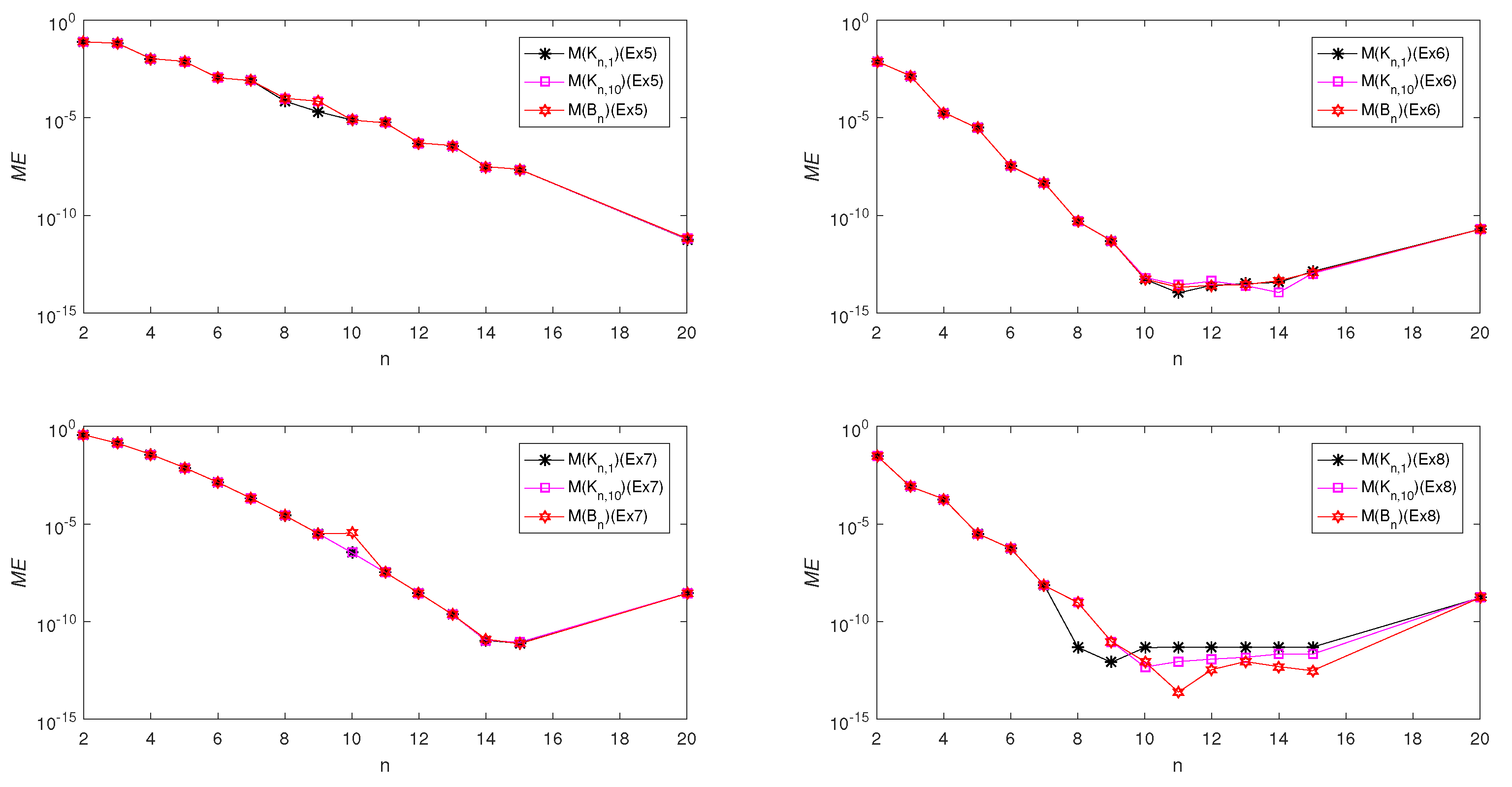
3. Test problems are conducted and theoretical results are justified with the obtained numerical results.

2. Asymptotic Rate of Convergence of Modified Bernstein–Kantorovich Operators

The Modified Bernstein–Kantorovich operators $K_{n,\alpha }\left(f;x\right)$ were used to approximate a function $f:\left[0,1\right]\to R$ (see Özarslan and Duman [37]) where,

$$K_{n,\alpha }\left(f;x\right)=\sum _{k=0}^n{P}_{n,k}\left(x\right)\underset{0}{\overset{1}{\int }}f\left(\frac{k+t^{\alpha }}{n+1}\right)dt,$$

(1)

and

$$P_{n,k}\left(x\right)=\left(\begin{array}{c}n\\ k\end{array}\right)x^k{\left(1-x\right)}^{n-k},$$

(2)

and $\alpha >0$ is constant. For $\alpha =1$ reduces to classical Bernstein–Kantorovich operator

$$K_n:=K_{n,1}\left(f;x\right)=\left(n+1\right)\sum _{k=0}^n{P}_{n,k}\left(x\right)\underset{\frac{k}{n+1}}{\overset{\frac{k+1}{n+1}}{\int }}f\left(t\right)dt.$$

(3)

Theorem 1.

(Theorem 2.3 in Özarslan and Duman [37]) For each $\alpha >0$ and every $f\in C\left[0,1\right]$ we have $K_{n,\alpha }\left(f\right)\rightrightarrows f$ on $\left[0,1\right],$ where the symbol ⇉ denotes the uniform convergence.

Lemma 1.

For each fixed $n\in N,\alpha >0$ and $x\in \left[0,1\right]$ we have

$$\underset{x\in \left[0,1\right]}{sup}\left|K_{n,\alpha }\left(\left(t-x\right);x\right)\right|\le \frac{\beta \left(\alpha \right)}{n+1},$$

(4)

$$\underset{x\in \left[0,1\right]}{sup}\left|K_{n,\alpha }\left({\left(t-x\right)}^2;x\right)\right|\le \frac{1}{{\left(n+1\right)}^2}\left(\frac{n}{4}+\sigma \left(\alpha \right)\right),$$

(5)

where,

$$\beta \left(\alpha \right)=\left\{\begin{array}{c}\frac{1}{\alpha +1}\mathit{if}0<\alpha <1,\\ \frac{\alpha }{\alpha +1}\mathit{if}\alpha \ge 1,\end{array}\right..$$

(6)

$$\sigma \left(\alpha \right)=\left\{\begin{array}{c}\frac{1}{2\alpha +1}\mathit{if}0<\alpha <1,\\ \frac{2{\alpha }^2}{\left(\alpha +1\right)\left(2\alpha +1\right)}\mathit{if}\alpha \ge 1.\end{array}\right.$$

(7)

Proof. 

From (1) it follows that

$$K_{n,\alpha }(t-x;x)=\frac{1}{n+1}\left(\frac{1}{\alpha +1}-x\right),$$

(8)

$$K_{n,\alpha }({\left(t-x\right)}^2;x)=\frac{1}{{\left(n+1\right)}^2}\left(nx\left(1-x\right)+\phi \left(\alpha ,x\right)\right),$$

(9)

where

$$\phi \left(\alpha ,x\right)=x^2-\frac{2x}{\alpha +1}+\frac{1}{2\alpha +1}.$$

(10)

For each fixed $n\in N,\alpha >0$ the inequality (4) is obtained from $\beta \left(\alpha \right)={\displaystyle \underset{x\in \left[0,1\right]}{max}}\left|\frac{1}{\alpha +1}-x\right|.$ The function $\phi \left(\alpha ,x\right)>0$ for $\alpha >0$ on $x\in \left[0,1\right].$ Further, ${\displaystyle \underset{x\in \left[0,1\right]}{min}}\phi \left(\alpha ,x\right)=$$\frac{{\alpha }^2}{{\left(\alpha +1\right)}^2\left(2\alpha +1\right)}$ occurring at $x=\frac{1}{\alpha +1}$ and ${\displaystyle \underset{x\in \left[0,1\right]}{max}}\phi \left(\alpha ,x\right)=$$\sigma \left(\alpha \right)$ occurring at the end points of the interval $\left[0,1\right].$ Furthermore, using that ${\displaystyle \underset{x\in \left[0,1\right]}{max}}\left(x\left(1-x\right)\right)=\frac{1}{4}$ yields (5). □

Next, we use the notations $∥q∥=$${\displaystyle \underset{x\in \left[0,1\right]}{sup}}$$\left|q\right|$ and ${∥q∥}_2={\left(\underset{0}{\overset{1}{\int }}{\left|q\left(x\right)\right|}^{2}dx\right)}^{\frac{1}{2}}$ to present the maximum norm for $q\in C\left[0,1\right]$ and $L^2-$norm of the function $q\in L^2\left[0,1\right].$ Further, we denote ${∥Y∥}_2=\sqrt{\left({\displaystyle \sum _{k=1}^n}{\left(Y\left(k\right)\right)}^2\right)}$ and ${∥P∥}_2=\sqrt{\rho \left(P^{T}P\right)}$ to present the discrete Euclidean norm of a vector $Y\in R^n$ and the spectral norm of a matrix $P\in R^{n\times n}$, respectively, where $\rho$ is the spectral radius and $P^T$ is the transpose of P. Voronowskaja [38] gave the asymptotic rate of convergence of the Bernstein operators

$$B_n\left(f;x\right)=\sum _{k=0}^n{P}_{n,k}\left(x\right)f\left(\frac{k}{n}\right),$$

(11)

using the linearity property of the Bernstein operators and Taylor formula at a point x as

$$\underset{n\to \infty }{lim}n\left[\left(B_n\left(f;x)\right)-f\left(x\right)\right)\right]=\frac{1}{2}x(1-x)f^{″}\left(x\right).$$

(12)

Based on the analogous approach in Voronowskaja [38] we give the asymptotic rate of convergence of the Modified Bernstein–Kantorovich operators by the next theorem.

Theorem 2.

If f is integrable in $\left[0,1\right],$ and admits a derivative of second order at some point $x\in \left[0,1\right]$ then

$$\underset{n\to \infty }{lim}n\left[K_{n,\alpha }(f;x)-f\left(x\right)\right]=\left(\frac{1}{\alpha +1}-x\right)f^{\prime }\left(x\right)+\frac{1}{2}x(1-x)f^{″}\left(x\right).$$

(13)

Additionally this limit is uniform if $f\in C^2\left[0,1\right]$, thus the rate of convergence of the operator $K_{n,\alpha }(f;x)$ to $f\left(x\right)$ is $O\left(\frac{1}{n}\right)$ for $x\in \left[0,1\right].$

Proof. 

Assume that f is integrable in $\left[0,1\right],$ and has second order derivative at a point $x\in \left[0,1\right]$ then from Taylor’s formula at x we have

$$f\left(t\right)=f\left(x\right)+\left(t-x\right)f^{\prime }\left(x\right)+\frac{{\left(t-x\right)}^2}{2}{f}^{″}\left(x\right)+{\left(t-x\right)}^{2}E\left(t-x\right),$$

(14)

and $E\left(u\right)\to 0$ as $u\to 0$ and E is integrable function on $\left[-x,1-x\right].$ Using the linearity property of the operators $K_{n,\alpha }$ and (8)–(10) we have

$$\begin{array}{ccc}\hfill K_{n,\alpha }\left(f;x\right)-f\left(x\right)& =& \frac{1}{n+1}\left(\frac{1}{\alpha +1}-x\right)f^{\prime }\left(x\right)\hfill \\ & & +\frac{1}{2{\left(n+1\right)}^2}\left(x^2-\frac{2x}{\alpha +1}+\frac{1}{2\alpha +1}+nx\left(1-x\right)\right)f^{″}\left(x\right)\hfill \\ & & +E\left(n,\alpha ,x\right),\hfill \end{array}$$

(15)

where,

$$E\left(n,\alpha ,x\right)=\sum _{k=0}^n{P}_{n,k}\left(x\right)\underset{0}{\overset{1}{\int }}{\left(\frac{k+t^{\alpha }}{n+1}-x\right)}^{2}E\left(\frac{k+t^{\alpha }}{n+1}-x\right)dt.$$

(16)

To show that the asymptotic rate of convergence is $O\left(\frac{1}{n}\right)$, it is sufficient to show that ${\displaystyle \underset{n\to \infty }{lim}}nE\left(n,\alpha ,x\right)=0$. Let $M_1={\displaystyle \underset{u\in \left[-x,1-x\right]}{sup}}\left|E\left(u\right)\right|$ and for arbitrary $\epsilon >0$ there exist ${\delta }_1>0$ such that $\left|E\left(u\right)\right|<\epsilon$ whenever $\left|u\right|<{\delta }_1$. For all $t\in \left[0,1\right]$ it follows that $\left|E\left(\frac{k+t^{\alpha }}{n+1}-x\right)\right|<\epsilon +M_1{\left(\frac{k+t^{\alpha }}{n+1}-x\right)}^2/{\delta }_1^2.$ Then, let

$${\gamma }_p\left(\alpha \right)=\prod _{k=1}^p(1+k\alpha ),p=1,2,3,4.$$

(17)

Using Lemma 1 estimation (5) gives

$$\begin{array}{ccc}\hfill \left|E\left(n,\alpha ,x\right)\right|& \le & \epsilon \left|K_{n,\alpha }\left({\left(t-x\right)}^2;x\right)\right|+\frac{M_1}{{\delta }_1^2}\left|K_{n,\alpha }\left({\left(t-x\right)}^4;x\right)\right|\hfill \\ & \le & \frac{\epsilon }{{\left(n+1\right)}^2}\left(\frac{n}{4}+\sigma \left(\alpha \right)\right)+\frac{M_1\tilde{M}\left(n,\alpha \right)}{{\delta }_1^2{\left(n+1\right)}^4{\gamma }_4\left(\alpha \right)},\hfill \end{array}$$

(18)

where, $\sigma \left(\alpha \right)$ is as given in (7) and $\tilde{M}\left(n,\alpha \right)={\displaystyle \underset{x\in \left[0,1\right]}{sup}}\left|Q\left(n,\alpha ,x\right)\right|.$ In addition for a fixed $\alpha$, $\tilde{M}\left(n,\alpha \right)$ is second degree polynomial in n and $Q\left(n,\alpha ,x\right)$ is

$$\begin{array}{ccc}\hfill Q\left(\alpha ,n,x\right)& =& 1+6\alpha +11{\alpha }^2+6{\alpha }^3\hfill \\ & & +(1+4\alpha )(-4{\gamma }_2\left(\alpha \right)+(1+3\alpha )(11+\alpha (17+2\alpha ))n)x\hfill \\ & & +\frac{{\gamma }_4\left(\alpha \right)}{{\gamma }_2\left(\alpha \right)}(6(1+\alpha )-(41+\alpha (87+22\alpha ))n+3{\gamma }_2\left(\alpha \right)n^2)x^2\hfill \\ & & -2\frac{{\gamma }_4\left(\alpha \right)}{{\gamma }_1\left(\alpha \right)}(2+n(-25+3\alpha (-5+n)+3n))x^3\hfill \\ & & +{\gamma }_4\left(\alpha \right)(1+n(-20+3n))x^4.\hfill \end{array}$$

(19)

It is obvious from (18) and (19) that for n large enough we have $\left|nE\left(\alpha ,n,x\right)\right|<\epsilon$ and using (15) we obtain (13). If $f\in C^2\left[0,1\right]$ then this limit is uniform, thus the rate of convergence of the operator $K_{n,\alpha }(f;x)$ to $f\left(x\right)$ is $O\left(\frac{1}{n}\right)$ for $x\in \left[0,1\right].$ □

Corollary 1.

If $f\in \left(C^{\lambda }\cap L^2\right)\left(\left[0,1\right]\right)$ for $\lambda \ge 2$ then

$$\begin{array}{ccc}\hfill \left|K_{n,\alpha }\left(f;x\right)-f\left(x\right)\right|& \le & \frac{∥f^{\prime }∥}{n+1}\left|\frac{1}{\alpha +1}-x\right|\hfill \end{array}$$

$$\begin{array}{ccc}& & +\frac{1}{2}\frac{∥f^{″}∥}{{\left(n+1\right)}^2}\left(nx\left(1-x\right)+\phi \left(\alpha ,x\right)\right),\hfill \end{array}$$

(20)

$$\begin{array}{ccc}\hfill \underset{x\in \left[0,1\right]}{sup}\left|K_{n,\alpha }\left(f;x\right)-f\left(x\right)\right|& \le & \frac{∥f^{\prime }∥}{n+1}\beta \left(\alpha \right)+\frac{∥f^{″}∥}{2{\left(n+1\right)}^2}\left(\frac{n}{4}+\sigma \left(\alpha \right)\right),\hfill \end{array}$$

(21)

$$\begin{array}{ccc}\hfill {∥K_{n,\alpha }\left(f\right)-f∥}_2& \le & {∥\frac{∥f^{\prime }∥}{n+1}\left(\frac{1}{\alpha +1}-x\right)∥}_2\hfill \\ & & +{∥\frac{∥f^{″}∥}{2{\left(n+1\right)}^2}\left(nx\left(1-x\right)+\phi \left(\alpha ,x\right)\right)∥}_2,\hfill \\ & =& \frac{∥f^{\prime }∥}{n+1}\tilde{\beta }\left(\alpha \right)+\frac{∥f^{″}∥}{2{\left(n+1\right)}^2}\tilde{\sigma }\left(n,\alpha \right),\hfill \end{array}$$

(22)

hold true where, $\phi \left(\alpha ,x\right)$ is the given function in (10)

$$\tilde{\beta }\left(\alpha \right)=\frac{\sqrt{1-\alpha +{\alpha }^2}}{(1+\alpha )\sqrt{3}},$$

(23)

$$\tilde{\sigma }\left(n,\alpha \right)=\frac{\sqrt{\frac{{\varphi }_1\left(\alpha \right)}{{\left({\gamma }_2\left(\alpha \right)\right)}^2}+\frac{{\varphi }_2\left(n,\alpha \right)}{{\gamma }_2\left(\alpha \right)}+n^2}}{\sqrt{30}},$$

(24)

$$\begin{array}{ccc}\hfill {\varphi }_1\left(\alpha \right)& =& 6+2\alpha \left(3+4\alpha \left(1+\alpha \left(-1+3\alpha \right)\right)\right),\hfill \end{array}$$

(25)

$$\begin{array}{ccc}\hfill {\varphi }_2\left(n,\alpha \right)& =& \left(3+\alpha \left(-1+6\alpha \right)\right)n,\hfill \end{array}$$

(26)

and $\beta \left(\alpha \right),\sigma \left(\alpha \right)$ are as given in (6) and (7), respectively, and ${\gamma }_2\left(\alpha \right)$ is the same as in (17).

Proof. 

The inequality (20) is the consequence of the Theorem 2. The proof of (21) is obtained by using (20), Lemma 1 and estimations (4) and (5). For $\alpha >0$ and $n\in N$ the proof of (22) follows from the integral values

$$\begin{array}{ccc}\hfill {\left(\underset{0}{\overset{1}{\int }}{\left|\frac{1}{\alpha +1}-x\right|}^{2}dx\right)}^{\frac{1}{2}}& =& \tilde{\beta }\left(\alpha \right),\hfill \\ \hfill {\left(\underset{0}{\overset{1}{\int }}{\left|nx\left(1-x\right)+\phi \left(\alpha ,x\right)\right|}^{2}dx\right)}^{\frac{1}{2}}& =& \tilde{\sigma }\left(\alpha ,n\right),\hfill \end{array}$$

given in (23), (24), respectively. □

3. Representation of the ${\mathit{K}}_{\mathit{n},\mathit{\alpha }}$ Operators and Discretization of First Kind Integral Equations

We consider the Fredholm integral equation of the first kind (FK1)

$$Tf=\underset{0}{\overset{1}{\int }}K\left(x,t\right)f\left(t\right)dt=g\left(x\right),0\le x\le 1,$$

(27)

and Volterra integral equations of the first kind (VK1)

$$\widehat{T}f=\underset{0}{\overset{x}{\int }}K\left(x,t\right)f\left(t\right)dt=g\left(x\right),0\le x\le 1,$$

(28)

where $g\left(x\right)$ is called the free term while $K\left(x,t\right)$ is called the kernel and $f\left(t\right)$ is the unknown function to be determined.

Definition 1.

(Groetsch [17,39]) By means of the singular value expansion (SVE) any square integrable kernel $K\left(x,t\right)$ can be written in the form

$$K\left(x,t\right)=\sum _{i=0}^{\infty }{\mu }_i{u}_i\left(x\right)v_i\left(t\right).$$

(29)

The functions $u_i,v_i$ are the singular functions of K and they are orthonormal with respect to the usual inner product $\left(.,.\right)$ and the number ${\mu }_i$ are the singular values of $K.$ For degenerate kernels the infinite sum (29) is replaced with the finite sum upto the rank of the kernel. The system $\left\{u_i,v_i;{\mu }_i\right\}$ is called the singular system of $K.$

Let $\mathsf{\Psi }:H_1\to H_2$ be a compact linear operator on a real Hilbert space $H_1$, taking values in a real Hilbert space $H_2$. The next theorem is known as the Picard’s theorem on the existence of the solutions of first kind equations.

Theorem 3.

(Theorem 1.2.6 in Groetsch [17]) Let $\mathsf{\Psi }:H_1\to H_2$ be a compact linear operator with singular system $\left\{u_i,v_i;{\mu }_i\right\}.$ In order that the equation $\mathsf{\Psi }f=g$ have a solution it is necessary and sufficient that $g\in N{\left({\mathsf{\Psi }}^{*}\right)}^{\perp }$ (orthogonal complement of the nullspace of the adjoint of $\mathsf{\Psi }$) and

$$\sum _{i=0}^{\infty }{\mu }_i^2{\left|\left(g,v_i\right)\right|}^2<\infty .$$

(30)

On the basis of Theorem 3 we consider the Hypothesis 1 as follows:

Hypothesis 1.

• The kernel $K\left(x,t\right)$ is continuous and square integrable function on $\left[0,1\right]\times \left[0,1\right].$
• $g\in C\left[0,1\right]$ and forFK1$g\in N{\left(T^{*}\right)}^{\perp }$ and forVK1$g\in N{\left({\widehat{T}}^{*}\right)}^{\perp }$, also the Picard’s condition (30) is satisfied.

Without loss of generality, the solution f of FK1 and VK1 denotes the pseudoinverse solution or the Moore-Penrose generalized inverse solution for FK1 and VK1

$$f=T^{†}g\mathrm{and}f={\widehat{T}}^{†}g,$$

(31)

respectively. Further, in order to determine the effect of $\alpha >0$ in the numerical solution we represent the Modified Bernstein–Kantorovich operators (1) for $0<\mu <1$ in the form

$$\begin{array}{ccc}\hfill K_{n,\alpha }\left(f;x\right)& =& \sum _{k=0}^n{P}_{n,k}\left(x\right)\left(\underset{0}{\overset{\mu }{\int }}f\left(\frac{k+t^{\alpha }}{n+1}\right)dt+\underset{\mu }{\overset{1}{\int }}f\left(\frac{k+t^{\alpha }}{n+1}\right)dt\right)\hfill \\ & =& \omega \sum _{k=0}^n{P}_{n,k}\left(x\right)\left(\frac{1}{\omega }\underset{0}{\overset{\mu }{\int }}f\left(\frac{k+t^{\alpha }}{n+1}\right)dt+\underset{\frac{k+{\mu }^{\alpha }}{n+1}}{\overset{\frac{k+1}{n+1}}{\int }}q\left(u\right)du\right),\hfill \end{array}$$

(32)

where

$$\begin{array}{ccc}\hfill q\left(u\right)& =& \left\{\begin{array}{c}f\left(u\right){\left(\left(n+1\right)u-k\right)}^{\frac{1-\alpha }{\alpha }}\mathit{if}\alpha \ne 1,\\ f\left(u\right)\mathit{if}\alpha =1,\end{array}\right.\hfill \end{array}$$

(33)

$$\begin{array}{ccc}\hfill \omega & =& \frac{\left(n+1\right)}{\alpha }.\hfill \end{array}$$

(34)

For the numerical solution of FK1 and VK1, we approximate the function f by using the Modified Bernstein–Kantorovich operators in (32). We obtain the following equation for FK1

$$\omega \sum _{k=0}^n\underset{0}{\overset{1}{\int }}K\left(x,t\right)P_{n,k}\left(t\right)\left(\frac{1}{\omega }\underset{0}{\overset{\mu }{\int }}f\left(\frac{k+t^{\alpha }}{n+1}\right)dt+\underset{\frac{k+{\mu }^{\alpha }}{n+1}}{\overset{\frac{k+1}{n+1}}{\int }}q\left(u\right)du\right)dt=g\left(x\right),$$

(35)

and for VK1 we get

$$\omega \sum _{k=0}^n\underset{0}{\overset{x}{\int }}K\left(x,t\right)P_{n,k}\left(t\right)\left(\frac{1}{\omega }\underset{0}{\overset{\mu }{\int }}f\left(\frac{k+t^{\alpha }}{n+1}\right)dt+\underset{\frac{k+{\mu }^{\alpha }}{n+1}}{\overset{\frac{k+1}{n+1}}{\int }}q\left(u\right)du\right)dt=g\left(x\right).$$

(36)

Subsequently we take the grid points $x_j=\frac{j}{n}+ϵ,$$j=0,1,\dots ,n-1$ and $x_n=1-ϵ$, where $0<ϵ<\frac{1}{2n}$. Then, the Equations (35) and (36) are transformed into algebraic systems of equations

$$AX=B,\mathrm{and}\widehat{A}X=B,$$

(37)

respectively, where the coefficient matrices A and $\widehat{A}$ have the entries

$$\begin{array}{ccc}\hfill {\left[A\right]}_{j+1,k+1}& =& \omega {\left[A_{*}\right]}_{j+1,k+1}=\omega \underset{0}{\overset{1}{\int }}K\left(x_j,t\right)P_{n,k}\left(t\right)dt,\hfill \end{array}$$

(38)

$$\begin{array}{ccc}\hfill {\left[\widehat{A}\right]}_{j+1,k+1}& =& \omega {\left[{\widehat{A}}_{*}\right]}_{j+1,k+1}=\omega \underset{0}{\overset{x_j}{\int }}K\left(x_j,t\right)P_{n,k}\left(t\right)dt,\hfill \end{array}$$

(39)

$j=0,1,\dots ,n,k=0,1,\dots ,n,$ and

$$\begin{array}{ccc}\hfill X\left(k+1\right)& =& \frac{1}{\omega }\underset{0}{\overset{\mu }{\int }}f\left(\frac{k+t^{\alpha }}{n+1}\right)dt+\underset{\frac{k+{\mu }^{\alpha }}{n+1}}{\overset{\frac{k+1}{n+1}}{\int }}q\left(u\right)du,k=0,1,\dots ,n,\hfill \end{array}$$

(40)

$$\begin{array}{ccc}\hfill B\left(j+1\right)& =& g\left(x_j\right),j=0,1,\dots ,n.\hfill \end{array}$$

(41)

$q\left(u\right)$ and $\omega$ are as given in (33) and (34), respectively. The coefficient matrices A and $\widehat{A}$ in (37) are ill-conditioned matrices and may be rank deficient or even singular matrices. Therefore, we consider the following minimum norm least squares problem for FK1

$$\underset{X\in S_1}{min}{∥X∥}_2,S_1=\left\{X\in R^{n+1}\mid {∥B-AX∥}_2=min\right\},$$

(42)

and for VK1

$$\underset{X\in S_2}{min}{∥X∥}_2,S_2=\left\{X\in R^{n+1}\mid {∥B-\widehat{A}X∥}_2=min\right\}.$$

(43)

Lemma 2.

The problems (42) and (43) have the unique minimum norm least squares solutions $X=A^{†}B$ and $X={\widehat{A}}^{†}B$ respectively.

Proof. 

Proof is analogous to the proof of Theorem 1.2.10 in Björck [40]. □

Convergence Analysis

By solving the algebraic systems (42) and (43) we get a numerical solution of the unknown (40) and denote this approximation by $X_n.$ Further, let us use $F_n$ to denote the obtained numerical approximation to f that is in the implicit form in $X_n$ and obtained by using the proposed approach. Substituting $F_n$ in (32) we get $K_{n,\alpha }\left(F_n;x\right)$ as

$$K_{n,\alpha }\left(F_n;x\right)=\omega \sum _{k=0}^n{P}_{n,k}\left(x\right)X_n\left(k+1\right),$$

(44)

Definition 2.

(Definition 1.4.2 in Björck [40]) The condition number of $U\in R^{m\times n}$ ($U\ne 0$) is

$$\kappa \left(U\right)={∥U^{†}∥}_2{∥U∥}_2=\frac{{\sigma }_1}{{\sigma }_{\tau }},$$

where $\tau =rank\left(U\right)$$\le min(m,n)$, and ${\sigma }_1\ge {\sigma }_2\ge ...\ge {\sigma }_{\tau }>0$ are the nonzero singular values of $U.$

Theorem 4.

ConsiderFK1andVK1in (27), (28), respectively, and assume that the conditions of theHypothesis Iare satisfied also the solution f belongs to $\left(C^{\lambda }\cap L^2\right)\left(\left[0,1\right]\right)$ for some $\lambda \ge 2$ then forFK1

$${∥K_{n,\alpha }\left(F_n\right)-f∥}_2\le W_1\left(n,\alpha ,f\right)+M_2{W}_2\left(n,\alpha ,f\right)\frac{\kappa \left(A_{*}\right)}{{∥A_{*}∥}_2},$$

(45)

and forVK1

$${∥K_{n,\alpha }\left(F_n\right)-f∥}_2\le W_1\left(n,\alpha ,f\right)+M_2{W}_2\left(n,\alpha ,f\right)\frac{\kappa \left({\widehat{A}}_{*}\right)}{{∥{\widehat{A}}_{*}∥}_2},$$

(46)

hold true where,

$$\begin{array}{ccc}\hfill W_1\left(n,\alpha ,f\right)& =& \frac{∥f^{\prime }∥}{n+1}\tilde{\beta }\left(\alpha \right)+\frac{∥f^{″}∥}{2{\left(n+1\right)}^2}\tilde{\sigma }\left(\alpha ,n\right),\hfill \end{array}$$

(47)

$$\begin{array}{ccc}\hfill W_2\left(n,\alpha ,f\right)& =& \frac{∥f^{\prime }∥}{n+1}\beta \left(\alpha \right)+\frac{∥f^{″}∥}{2{\left(n+1\right)}^2}\left(\frac{n}{4}+\sigma \left(\alpha \right)\right),\hfill \end{array}$$

(48)

and $\beta \left(\alpha \right),$$\sigma \left(\alpha \right),\tilde{\beta }\left(\alpha \right)$ and $\tilde{\sigma }\left(\alpha ,n\right)$ are given in (6), (7), (23) and (24) respectively. Furthermore, $M_2={∥S∥}_2$ where $S(j+1)={\displaystyle \underset{t\in \left[0,1\right]}{sup}}\left|K\left(x_j,t\right)\right|$, $x_j=\frac{j}{n}+ϵ,$ $j=0,1,\dots ,n-1$ and $x_n=1-ϵ$, and $0<ϵ<\frac{1}{2n}$. Further, $K_{n,\alpha }\left(F_n;x\right)$ is the approximate solution obtained by the proposed method and $A_{*}$ and ${\widehat{A}}_{*}$ are given in (38) and (39), respectively.

Proof. 

For FK1 it follows that

$${∥K_{n,\alpha }\left(F_n\right)-f∥}_2\le {∥K_{n,\alpha }\left(f\right)-f∥}_2+{∥K_{n,\alpha }\left(F_n\right)-K_{n,\alpha }\left(f\right)∥}_2.$$

(49)

Based on Corollary 1 and the estimation (22) and taking (47), we obtain

$${∥K_{n,\alpha }\left(f\right)-f∥}_2\le W_1\left(n,\alpha ,f\right).$$

(50)

Next let $\overline{X}\left(k+1\right)=X_n\left(k+1\right)-X\left(k+1\right)$ for $k=0,1,\dots ,n$ from (32) and (44) and using that ${\displaystyle \sum _{k=0}^n}{P}_{n,k}\left(x\right)=1$ gives

$$\begin{array}{ccc}\hfill {∥K_{n,\alpha }\left(F_n\right)-K_{n,\alpha }\left(f\right)∥}_2& =& {\left(\underset{0}{\overset{1}{\int }}{\left|\omega \sum _{k=0}^n{P}_{n,k}\left(x\right)\overline{X}\left(k+1\right)\right|}^{2}dx\right)}^{\frac{1}{2}}\hfill \\ & \le & \omega {\left(\sum _{k=1}^{n+1}{\left(\overline{X}\left(k\right)\right)}^2\right)}^{\frac{1}{2}}{\left(\underset{0}{\overset{1}{\int }}{\left|\sum _{k=0}^n{P}_{n,k}\left(x\right)\right|}^{2}dx\right)}^{\frac{1}{2}}.\hfill \end{array}$$

(51)

It follows that

$${∥K_{n,\alpha }\left(F_n\right)-K_{n,\alpha }\left(f\right)∥}_2\le \omega {∥\overline{X}∥}_2.$$

(52)

From Theorem 1, the operator $K_{n,\alpha }\left(f;x\right)$ uniformly converges to f for any $f\in C\left[0,1\right]$ and for any computationally acceptable small $\epsilon >0,$

$$\left|K_{n,\alpha }\left(f;x\right)-f\left(x\right)\right|<\epsilon +\frac{2∥f∥}{{\delta }_1^2}{K}_{n,\alpha }({\left(t-x\right)}^2;x),$$

where, as usual, ${\delta }_1$ comes from the uniform continuity of the function $f$$\in \left[0,1\right]$ and $K_{n,\alpha }({\left(t-x\right)}^2;x)$ is given in (9) (see Özarslan and Duman [37]). Therefore, for the numerical solution of FK1 and VK1 equations in (27), and (28) in accordance we assume

$$\begin{array}{ccc}\hfill \underset{0}{\overset{1}{\int }}K\left(x,t\right)K_{n,\alpha }\left(f;t\right)dt& =& g\left(x\right),0\le x\le 1,\hfill \end{array}$$

(53)

$$\begin{array}{ccc}\hfill \underset{0}{\overset{x}{\int }}K\left(x,t\right)K_{n,\alpha }\left(f;t\right)dt& =& g\left(x\right),0\le x\le 1,\hfill \end{array}$$

(54)

respectively. If we substitute $F_n\left(x\right)$ instead of $f\left(x\right)$ in (53), (54) we get new function $\widehat{g}\left(x\right)$ on the right sides of these equations accordingly,

$$\begin{array}{ccc}\hfill \underset{0}{\overset{1}{\int }}K\left(x,t\right)K_{n,\alpha }\left(F_n;t\right)dt& =& \widehat{g}\left(x\right),0\le x\le 1,\hfill \end{array}$$

(55)

$$\begin{array}{ccc}\hfill \underset{0}{\overset{x}{\int }}K\left(x,t\right)K_{n,\alpha }\left(F_n;t\right)dt& =& \widehat{g}\left(x\right),0\le x\le 1.\hfill \end{array}$$

(56)

Thus, for FK1 using (53) and (55) and by taking the grid points $x_j=\frac{j}{n}+ϵ,$ $j=0,1,\dots ,n-1$ and $x_n=1-ϵ$, where $0<ϵ<\frac{1}{2n}$ we obtain the algebraic system

$$A\overline{X}=\overline{B},\overline{B}\left(j+1\right)=\widehat{g}\left(x_j\right)-g\left(x_j\right),j=0,1,\dots ,n.$$

(57)

The minimum norm solution of the least squares problem for (57) is

$$\overline{X}=A^{†}\overline{B}.$$

(58)

Thus

$$\omega {∥\overline{X}∥}_2\le \omega {∥A^{†}∥}_2{∥\overline{B}∥}_2={∥A_{*}^{†}∥}_2{∥\overline{B}∥}_2,$$

(59)

and for VK1

$$\omega {∥\overline{X}∥}_2\le \omega {∥{\widehat{A}}^{†}∥}_2{∥\overline{B}∥}_2={∥{\widehat{A}}_{*}^{†}∥}_2{∥\overline{B}∥}_2.$$

(60)

Next, consider FK1 and let $\widehat{g}\left(x\right)=\underset{0}{\overset{1}{\int }}K\left(x,t\right)K_{n,\alpha }\left(f;t\right)dt$ and $g\left(x\right)=\underset{0}{\overset{1}{\int }}K\left(x,t\right)f\left(t\right)dt,$ then it follows that

$$\widehat{g}\left(x\right)-g\left(x\right)=\underset{0}{\overset{1}{\int }}K\left(x,t\right)\left(K_{n,\alpha }\left(f;t\right)-f\left(t\right)\right)dt,$$

(61)

then using Corollary 1 and estimation (21) and (57) and (61) and taking $S(j+1)={\displaystyle \underset{t\in \left[0,1\right]}{sup}}\left|K\left(x_j,t\right)\right|$ for $j=0,1,\dots ,n$ and $M_2={∥S∥}_2$ and using (48) we get

$$\begin{array}{ccc}\hfill {\left(\sum _{j=0}^n{\left|\left(\widehat{g}\left(x_j\right)-g\left(x_j\right)\right)\right|}^2\right)}^{\frac{1}{2}}& =& {\left(\sum _{j=0}^n{\left|\underset{0}{\overset{1}{\int }}K\left(x_j,t\right)\left(K_{n,\alpha }\left(f;t\right)-f\left(t\right)\right)dt\right|}^2\right)}^{\frac{1}{2}}\hfill \\ & \le & {\left(\sum _{j=0}^n{\left(S(j+1)\right)}^2\right)}^{\frac{1}{2}}\underset{t\in \left[0,1\right]}{sup}\left|K_{n,\alpha }\left(f;t\right)-f\left(t\right)\right|\hfill \\ & \le & M_2{W}_2\left(n,\alpha ,f\right).\hfill \end{array}$$

(62)

Substituting (62) into (59) and the obtained result in (52) gives

$${∥K_{n,\alpha }\left(F_n\right)-K_{n,\alpha }\left(f\right)∥}_2\le M_2{W}_2\left(n,\alpha ,f\right){∥A_{*}^{†}∥}_2.$$

(63)

Further, using the estimations (50) and (63) in (49) and also from $\kappa \left(A_{*}\right)={∥A_{*}^{†}∥}_2{∥A_{*}∥}_2$ we get (45). Analogously, for VK1 it follows that

$$\widehat{g}\left(x\right)-g\left(x\right)=\underset{0}{\overset{x}{\int }}K\left(x,t\right)\left(K_{n,\alpha }\left(f;t\right)-f\left(t\right)\right)dt.$$

(64)

Using Corollary 1 and estimation (21) and taking (48), we obtain

$$\begin{array}{ccc}\hfill {\left(\sum _{j=0}^n{\left|\left(\widehat{g}\left(x_j\right)-g\left(x_j\right)\right)\right|}^2\right)}^{\frac{1}{2}}& =& {\left(\sum _{j=0}^n{\left|\underset{0}{\overset{x_j}{\int }}K\left(x_j,t\right)\left(K_{n,\alpha }\left(f;t\right)-f\left(t\right)\right)dt\right|}^2\right)}^{\frac{1}{2}}\hfill \\ & \le & {\left(\sum _{j=0}^n{\left(S(j+1)\right)}^2\right)}^{\frac{1}{2}}\underset{t\in \left[0,1\right]}{sup}\left|K_{n,\alpha }\left(f;t\right)-f\left(t\right)\right|\hfill \\ & \le & M_2{W}_2\left(n,\alpha ,f\right).\hfill \end{array}$$

(65)

Next, substituting (65) in (60) and the obtained result in (52) we get

$${∥K_{n,\alpha }\left(F_n\right)-K_{n,\alpha }\left(f\right)∥}_2\le M_2{W}_2\left(n,\alpha ,f\right){∥{\widehat{A}}_{*}^{†}∥}_2.$$

(66)

Therefore, using the estimations (50) and (66) in (49) follows (46). □

Remark 1.

If the matrix A in (38) and the matrix $\widehat{A}$ in (39) are invertible then $A^{†}=A^{-1}$ and ${\widehat{A}}^{†}={\widehat{A}}^{-1}$and the inequalities (45) and (46) hold true.

4. Regularized Numerical Solution

The numerical solution of the general least squares problems (42) and (43) may be extremely difficult because the solution is very sensitive to the perturbations of the coefficient matrices A and $\widehat{A}$ and the right side vector B. This is reflected in the fact that $\kappa \left(A\right),$ and $\kappa \left(\widehat{A}\right)$ are very large and increases as n increases which is the degree of the constructed polynomial by the Modified Bernstein–Kantorovich operator used for the approximation of the solution. High condition numbers of the matrices A and $\widehat{A}$ cause rounding errors that prevent the computation of an accurate numerical solution of the problems (42) and (43), respectively. Moreover, the obtained discrete problems are always perturbed by approximations such as the integrals given as the entries of A and $\widehat{A}$ are evaluated numerically. Therefore, even if we were able to solve the discrete algebraic problems (42) and (43) without rounding errors we would not obtain a “smooth” solution because of the oscillations in the singular vectors. By a smooth solution we mean “a solution which has some useful properties in common with the exact solution to the underlying and unknown unperturbed problem” as stated in Hansel [41]. Furthermore, the function g is typically a measured or observed quantity and hence, in practice, the true g is not available to us. On one hand, the estimate $g_{\delta }$ of g satisfying ${∥g_{\delta }-g∥}_2\le \delta$ and $\delta$ is the priori error level is known(see Tikhonov [15] and [16] and Groetsch [17]). Therefore, we consider the following regularized problems for the Fredholm integral equation of the first kind (RFK1) (see Tikhonov [15,16] and Groetsch [17])

$$\underset{0}{\overset{1}{\int }}K\left(x,t\right)f_{\eta }^{\delta }\left(t\right)dt+\eta \left(\delta \right)f_{\eta }^{\delta }\left(x\right)=g_{\delta }\left(x\right),0\le x\le 1,$$

(67)

and Volterra integral equations of the first kind (RVK1)

$$\underset{0}{\overset{x}{\int }}K\left(x,t\right)f_{\eta }^{\delta }\left(t\right)dt+\eta \left(\delta \right)f_{\eta }^{\delta }\left(x\right)=g_{\delta }\left(x\right),0\le x\le 1.$$

(68)

It is clear that (67) and (68) are second kind Fredholm and Volterra integral equations, respectively. For the numerical solution of RFK1 and RVK1 by the proposed method $M\left(K_{n,\alpha }\right)$ we take the grid points $x_j=\frac{j}{n}+ϵ,$ $j=0,1,\dots ,n-1$ and $x_n=1-ϵ$, where $0<ϵ<\frac{1}{2n}$ and is sufficiently small number also $\eta \left(\delta \right)>0$ is called the regularization parameter. We assume the following algebraic equations for RFK1

$$\omega \sum _{k=0}^n\left(\underset{0}{\overset{1}{\int }}K\left(x_j,t\right)K_{n,\alpha }(f_{\eta }^{\delta };t)dt\right)+\omega \eta \left(\delta \right)X_{\eta }^{\delta }\left(j+1\right)=g_{\delta }\left(x_j\right),$$

(69)

and for RVK1

$$\omega \sum _{k=0}^n\left(\underset{0}{\overset{x_j}{\int }}K\left(x_j,t\right)K_{n,\alpha }(f_{\eta }^{\delta };t)dt\right)+\omega \eta \left(\delta \right)X_{\eta }^{\delta }\left(j+1\right)=g_{\delta }\left(x_j\right),$$

(70)

for $j=0,1,\dots ,n,$$k=0,1,\dots ,n.$ Then, the discrete regularized Equations (69) and (70) can be presented in matrix form

$$\tilde{A}{X}_{\eta }^{\delta }=\tilde{B},\tilde{\widehat{A}}{X}_{\eta }^{\delta }=\tilde{B},$$

(71)

for the RFK1 and for the RVK1 respectively where,

$$\begin{array}{ccc}\hfill X_{\eta }^{\delta }\left(k+1\right)& =& \frac{1}{\omega }\underset{0}{\overset{\mu }{\int }}{f}_{\eta }^{\delta }\left(\frac{k+t^{\alpha }}{n+1}\right)dt+\underset{\frac{k+{\mu }^{\alpha }}{n+1}}{\overset{\frac{k+1}{n+1}}{\int }}{q}_{\eta }^{\delta }\left(u\right)du,k=0,1,\dots ,n,\hfill \end{array}$$

(72)

$$\begin{array}{ccc}\hfill q_{\eta }^{\delta }\left(u\right)& =& \left\{\begin{array}{c}{f}_{\eta }^{\delta }\left(u\right){\left(\left(n+1\right)u-k\right)}^{\frac{1-\alpha }{\alpha }}\mathit{if}\alpha \ne 1,\\ f_{\eta }^{\delta }\left(u\right)\mathit{if}\alpha =1.\end{array}\right.\hfill \end{array}$$

(73)

and the vector $\tilde{B}\in R^{n+1}$

$$\tilde{B}\left(j+1\right)=g_{\delta }\left(x_j\right),j=0,1,\dots ,n.$$

(74)

which can be written as $\tilde{B}=B+\Delta B$ such that $\Delta B$ is the priori error level $∥\Delta B∥\le \delta .$ Furthermore, $\tilde{A}=A+\Delta A$ where A is the matrix in (38) and $\Delta A=\omega \eta \left(\delta \right)I+{\Delta }_{1}A,$ with the addition of diagonal matrix $\omega \eta \left(\delta \right)I$ and ${\Delta }_{1}A$ which is the defect matrix of the numerical errors of the computation of the integrals in (69) with a predescribed error ${\delta }^{*}={\delta }^{*}\left(\delta \right)\ge 0,$ depending on $\delta .$ Analogously, $\tilde{\widehat{A}}=\widehat{A}+\Delta \widehat{A}$ and $\widehat{A}$ is as in (39) and the matrix $\Delta \widehat{A}$$=\omega \eta \left(\delta \right)I+{\Delta }_1\widehat{A}$ has the defect matrix ${\Delta }_1\widehat{A}$ of the numerical errors of the computed integrals in (70) with a predescribed error ${\delta }^{*}={\delta }^{*}\left(\delta \right)\ge 0.$ Therefore, it is possible to choose $\eta \left(\delta \right),{\delta }^{*}$ such that ${∥\Delta A∥}_2\le h$ and ${∥\Delta \widehat{A}∥}_2\le h.$ Clearly, the numbers h and $\delta$ are estimates of the errors of the approximate data $\left(\tilde{A},\tilde{B}\right),\left(\tilde{\widehat{A}},\tilde{B}\right)$ of the problem (37) for FK1 and VK1, respectively, with the exact data $\left(A,B\right),\left(\widehat{A},B\right)$ accordingly. Thus, the given regularized systems (71) uses h and $\delta$ explicitly. For the implementation of the approach we have taken $\eta \left(\delta \right)=\delta$. In this connection, about the remarks on choosing the regularization parameter using the quasi-optimality and ratio criterion, see Bakushinskii [42] and for the data errors and an error estimation for ill-posed problems see Yagola et al. [43]. Next, we consider the following general least squares problem for RFK1

$$\underset{X_{\eta }^{\delta }\in {\tilde{S}}_1}{min}{∥X_{\eta }^{\delta }∥}_2,{\tilde{S}}_1=\left\{X_{\eta }^{\delta }\in R^{n+1}\mid {∥\tilde{B}-\tilde{A}{X}_{\eta }^{\delta }∥}_2=min\right\},$$

(75)

and for RVK1

$$\underset{X_{\eta }^{\delta }\in {\tilde{S}}_2}{min}{∥X_{\eta }^{\delta }∥}_2,{\tilde{S}}_2=\left\{X_{\eta }^{\delta }\in R^{n+1}\mid {∥\tilde{B}-\tilde{\widehat{A}}{X}_{\eta }^{\delta }∥}_2=min\right\}.$$

(76)

Theorem 5.

(Theorem 1.4.2 in Björck [40]) If $rank(U+\Delta U)=rank\left(U\right)$ and $\tilde{\eta }={∥U^{†}∥}_2{∥\Delta U∥}_2$ < 1 then

$${∥{\left(U+\Delta U\right)}^{†}∥}_2\le \frac{1}{1-\tilde{\eta }}{∥U^{†}∥}_2.$$

Theorem 6.

(Theorem 1.4.6 in Björck [40]) Assume that $rank(U+\Delta U)=rank\left(U\right)$ and let

$$\frac{{∥\Delta U∥}_2}{{∥U∥}_2}\le {ϵ}_U,\frac{{∥\Delta B∥}_2}{{∥B∥}_2}\le {ϵ}_B.$$

(77)

Then if $\tilde{\eta }=$$\kappa \left(U\right){ϵ}_U<1$ the perturbations $\Delta X$ and $\Delta r$ in the least squares solution X and the residual $r=B-UX$ satisfy

$$\begin{array}{ccc}\hfill {∥\Delta X∥}_2& \le & \frac{\kappa \left(U\right)}{1-\tilde{\eta }}\left({ϵ}_U{∥X∥}_2+{ϵ}_B\frac{{∥B∥}_2}{{∥U∥}_2}+{ϵ}_U\kappa \left(U\right)\frac{{∥r∥}_2}{{∥U∥}_2}\right)\hfill \end{array}$$

$$\begin{array}{ccc}& & +{ϵ}_U\kappa \left(U\right){∥X∥}_2,\hfill \end{array}$$

(78)

$$\begin{array}{ccc}\hfill {∥\Delta r∥}_2& \le & {ϵ}_U{∥X∥}_2{∥U∥}_2+{ϵ}_B{∥B∥}_2+{ϵ}_U\kappa \left(U\right){∥r∥}_2.\hfill \end{array}$$

(79)

Let $X_{\eta ,n}^{\delta }$ denote the minimum norm solution obtained by solving the general least squares problems (75) and (76). Further, $F_{\eta ,n}^{\delta }$ denote the obtained approximation to function $f_{\eta }^{\delta }$ appearing implicitly in (72). Substituting $F_{\eta ,n}^{\delta }$ in (32) we get $K_{n,\alpha }\left(F_{\eta ,n}^{\delta };x\right)$ as

$$K_{n,\alpha }\left(F_{\eta ,n}^{\delta };x\right)=\omega \sum _{k=0}^n{P}_{n,k}\left(x\right)X_{\eta ,n}^{\delta }\left(k+1\right).$$

(80)

We also present the residual error of the obtained algebraic linear system (37) for FK1 by $r=B-AX$ ( $r=B-\widehat{A}X$ for VK1). The regularized residual error of the system (71) for RFK1 is $r_{\eta }^{\delta }=\tilde{B}-\tilde{A}{X}_{\eta }^{\delta }$ ( $r_{\eta }^{\delta }=\tilde{B}-\tilde{\widehat{A}}{X}_{\eta }^{\delta }$ for RVK1). Furthermore, the corresponding numerical calculation of the regularized residual error is $r_{\eta ,n}^{\delta }=\tilde{B}-\tilde{A}{X}_{\eta ,n}^{\delta }$ ( $r_{\eta ,n}^{\delta }=\tilde{B}-\tilde{\widehat{A}}{X}_{\eta ,n}^{\delta }$) accordingly. Next, the following priory bound for the error of the approximation follows.

Theorem 7.

Assume that the conditions ofHypothesis Iare satisfied and the solution $f_{\eta }^{\delta }$ of (67)belongs to $\left(C^{\lambda }\cap L^2\right)\left(\left[0,1\right]\right)$ for some $\lambda \ge 2.$ Consider the regularized linear system $\tilde{A}{X}_{\eta }^{\delta }=\tilde{B}$ given in (71) where $\tilde{A}=A+\Delta A$ and A is the matrix in (38) and ${∥\Delta A∥}_2\le h$. Furthermore, $\tilde{B}=B+\Delta B$ as in (74) and B is the vector in (41) and ${∥\Delta B∥}_2\le \delta .$ Additionally $X_{\eta }^{\delta }=X+\Delta X$ and $r_{\eta }^{\delta }=r+\Delta r$ and let $S(j+1)={\displaystyle \underset{t\in \left[0,1\right]}{sup}}\left|K\left(x_j,t\right)\right|$ for $x_j=\frac{j}{n}+ϵ,$ $j=0,1,\dots ,n-1$ and $x_n=1-ϵ$, where $0<ϵ<\frac{1}{2n}$ and $M_2={∥S∥}_2.$ Further,

$$\frac{{∥\Delta A∥}_2}{{∥A∥}_2}\le \frac{h}{{∥A∥}_2}={ϵ}_A,\frac{{∥\Delta B∥}_2}{{∥B∥}_2}\le \frac{\delta }{{∥B∥}_2}={ϵ}_B.$$

(81)

If $rank\left(\tilde{A}\right)=rank\left(A\right)$ and $\tilde{\eta }=$$\kappa \left(A\right){ϵ}_A<1$ then

$$\begin{array}{ccc}\hfill {∥K_{n,\alpha }\left(F_{\eta ,n}^{\delta }\right)-f_{\eta }^{\delta }∥}_2& \le & W_1\left(n,\alpha ,f_{\eta }^{\delta }\right)\hfill \\ & & +\frac{M_2{W}_2\left(n,\alpha ,f_{\eta }^{\delta }\right)+\eta \left(\delta \right)W_3\left(n,f_{\eta }^{\delta }\right)}{1-\tilde{\eta }}\frac{\kappa \left(A_{*}\right)}{{∥A_{*}∥}_2},\hfill \end{array}$$

(82)

$$\begin{array}{ccc}\hfill {∥X-X_{\eta ,n}^{\delta }∥}_2& \le & \frac{\kappa \left(A\right)}{\left(1-\tilde{\eta }\right){∥A∥}_2}\left(h{∥X∥}_2+\delta +{ϵ}_A\kappa \left(A\right){∥r∥}_2\right)+{ϵ}_A\kappa \left(A\right){∥X∥}_2\hfill \end{array}$$

$$\begin{array}{ccc}& & +\frac{M_2{W}_2\left(n,\alpha ,f_{\eta }^{\delta }\right)+\eta \left(\delta \right)W_3\left(n,f_{\eta }^{\delta }\right)}{1-\tilde{\eta }}\frac{\kappa \left(A\right)}{{∥A∥}_2},\hfill \\ \hfill {∥r-r_{\eta ,n}^{\delta }∥}_2& \le & h{∥X∥}_2+\delta +{ϵ}_A\kappa \left(A\right){∥r∥}_2\hfill \end{array}$$

(83)

$$\begin{array}{ccc}& & +\left(1+{ϵ}_A\right)\frac{M_2{W}_2\left(n,\alpha ,f_{\eta }^{\delta }\right)+\eta \left(\delta \right)W_3\left(n,f_{\eta }^{\delta }\right)}{1-\tilde{\eta }}\kappa \left(A\right),\hfill \end{array}$$

(84)

hold true where, $\eta \left(\delta \right)$ is the regularization parameter and $W_1\left(n,\alpha ,f_{\eta }^{\delta }\right),$$W_2\left(n,\alpha ,f_{\eta }^{\delta }\right)$ are as in (47) and (48), respectively. Furthermore, $W_3\left(n,f_{\eta }^{\delta }\right)=\frac{1}{\sqrt{n+1}}∥\frac{d{f}_{\eta }^{\delta }}{dx}∥$ and $A,$$A_{*}$ are as given in (38).

Proof. 

For RFK1, it follows that

$${∥K_{n,\alpha }\left(F_{\eta ,n}^{\delta }\right)-f_{\eta }^{\delta }∥}_2\le {∥K_{n,\alpha }\left(f_{\eta }^{\delta }\right)-f_{\eta }^{\delta }∥}_2+{∥K_{n,\alpha }\left(F_{\eta ,n}^{\delta }\right)-K_{n,\alpha }\left(f_{\eta }^{\delta }\right)∥}_2.$$

(85)

Based on Corollary 1 and the estimation (22) by replacing f with $f_{\eta }^{\delta }$ in estimation (22) and in (47) we obtain

$${∥K_{n,\alpha }\left(f_{\eta ,n}^{\delta }\right)-f_{\eta }^{\delta }∥}_2\le W_1\left(n,\alpha ,f_{\eta }^{\delta }\right).$$

(86)

Let ${\overline{X}}_{\eta }^{\delta }=X_{\eta ,n}^{\delta }-X_{\eta }^{\delta }$ then from (32) and (44) and using that ${\displaystyle \sum _{k=0}^n}{P}_{n,k}\left(x\right)=1,$ follows

$$\begin{array}{ccc}\hfill {∥K_{n,\alpha }\left(F_{\eta ,n}^{\delta }\right)-K_{n,\alpha }\left(f_{\eta }^{\delta }\right)∥}_2& =& {\left(\underset{0}{\overset{1}{\int }}{\left|\omega \sum _{k=0}^n{P}_{n,k}\left(x\right){\overline{X}}_{\eta }^{\delta }\left(k+1\right)\right|}^{2}dx\right)}^{\frac{1}{2}}\hfill \\ & \le & \omega {\left(\sum _{k=0}^n{\left({\overline{X}}_{\eta }^{\delta }\left(k+1\right)\right)}^2\right)}^{\frac{1}{2}}{\left(\underset{0}{\overset{1}{\int }}{\left|\sum _{k=0}^n{P}_{n,k}\left(x\right)\right|}^{2}dx\right)}^{\frac{1}{2}}\hfill \\ & =& \omega {∥{\overline{X}}_{\eta }^{\delta }∥}_2,\hfill \end{array}$$

(87)

where

$$\begin{array}{ccc}\hfill {\overline{X}}_{\eta }^{\delta }\left(k+1\right)& =& \frac{1}{\omega }\underset{0}{\overset{\mu }{\int }}\left(F_{\eta ,n}^{\delta }\left(\frac{k+t^{\alpha }}{n+1}\right)-f_{\eta }^{\delta }\left(\frac{k+t^{\alpha }}{n+1}\right)\right)dt\hfill \\ & & +\underset{\frac{k+{\mu }^{\alpha }}{n+1}}{\overset{\frac{k+1}{n+1}}{\int }}\left(F_{\eta ,n}^{\delta }\left(u\right)-f_{\eta }^{\delta }\left(u\right)\right){\left(\left(n+1\right)u-k\right)}^{\frac{1-\alpha }{\alpha }}du.\hfill \end{array}$$

(88)

For the numerical solution of RFK1 in (67) we use the grid points $x_j=\frac{j}{n}+ϵ,$ $j=0,1,\dots ,n-1$ and $x_n=1-ϵ$, where $0<ϵ<\frac{1}{2n}.$ We assume

$$\underset{0}{\overset{1}{\int }}K\left(x_j,t\right)K_{n,\alpha }\left(f_{\eta }^{\delta };t\right)dt+\omega \eta \left(\delta \right)X_{\eta }^{\delta }\left(j+1\right)=g_{\delta }\left(x_j\right),$$

(89)

where $\omega X_{\eta }^{\delta }\left(j+1\right)$ gives the average value of $f_{\eta }^{\delta }$ over the interval $\left[\frac{j}{n+1},\frac{j+1}{n+1}\right].$ If we substitute $F_{\eta ,n}^{\delta }$ instead of $f_{\eta }^{\delta }$ in (89) we get a new function ${\widehat{g}}_{\delta }$ on the right side of this equation

$$\underset{0}{\overset{1}{\int }}K\left(x_j,t\right)K_{n,\alpha }\left(F_{\eta ,n}^{\delta };t\right)dt+\omega \eta \left(\delta \right)X_{\eta ,n}^{\delta }\left(j+1\right)={\widehat{g}}_{\delta }\left(x_j\right).$$

(90)

Thus, for RFK1 from (89) and (90) we obtain

$$\tilde{A}{\overline{X}}_{\eta }^{\delta }=\overline{\tilde{B}},\mathrm{and}\overline{\tilde{B}}\left(j+1\right)={\widehat{g}}_{\delta }\left(x_j\right)-g_{\delta }\left(x_j\right),j=0,1,\dots ,n,$$

(91)

where, ${\overline{X}}_{\eta }^{\delta }$ is as given in (88). The general least squares problem of (91) has the minimum norm solution

$${\overline{X}}_{\eta }^{\delta }={\tilde{A}}^{†}\overline{\tilde{B}}.$$

(92)

Thus,

$$\begin{array}{ccc}\hfill {∥{\overline{X}}_{\eta }^{\delta }∥}_2& \le & {∥{\tilde{A}}^{†}∥}_2{∥\overline{\tilde{B}}∥}_2,\hfill \end{array}$$

(93)

$$\begin{array}{ccc}\hfill \omega {∥{\overline{X}}_{\eta }^{\delta }∥}_2& \le & {∥{\tilde{A}}_{*}^{†}∥}_2{∥\overline{\tilde{B}}∥}_2.\hfill \end{array}$$

(94)

Then, let ${\widehat{g}}_{\delta }\left(x_j\right)=\underset{0}{\overset{1}{\int }}K\left(x_j,t\right)K_{n,\alpha }\left(f_{\eta }^{\delta };t\right)dt+$$\omega \eta \left(\delta \right)X_{\eta }^{\delta }\left(j+1\right)$ and $g_{\delta }\left(x_j\right)=\underset{0}{\overset{1}{\int }}K\left(x_j,t\right)$$f_{\eta }^{\delta }\left(t\right)dt+$$\eta \left(\delta \right)f_{\eta }^{\delta }\left(x_j\right)$ for $j=0,1,\dots ,n$ it follows that

$$\begin{array}{ccc}\hfill {\widehat{g}}_{\delta }\left(x_j\right)-g_{\delta }\left(x_j\right)& =& \underset{0}{\overset{1}{\int }}K\left(x_j,t\right)\left(K_{n,\alpha }\left(f_{\eta }^{\delta };t\right)-f_{\eta }^{\delta }\left(t\right)\right)dt\hfill \\ & & +\eta \left(\delta \right)\left(\omega X_{\eta }^{\delta }\left(j+1\right)-f_{\eta }^{\delta }\left(x_j\right)\right).\hfill \end{array}$$

(95)

From the assumption that $f_{\eta }^{\delta }\in \left(C^{\lambda }\cap L^2\right)\left(\left[0,1\right]\right)$ for some $\lambda \ge 2$ it follows that

${\displaystyle \underset{0\le j\le n}{sup}}\left|\omega X_{\eta }^{\delta }\left(j+1\right)-f_{\eta }^{\delta }\left(x_j\right)\right|$$\le \frac{1}{n+1}∥\frac{d{f}_{\eta }^{\delta }}{dx}∥.$ Let $W_3\left(n,f_{\eta }^{\delta }\right)=\frac{1}{\sqrt{n+1}}∥\frac{d{f}_{\eta }^{\delta }}{dx}∥$, by taking

$S(j+1)={\displaystyle \underset{t\in \left[0,1\right]}{sup}}\left|K\left(x_j,t\right)\right|$ for $j=0,1,\dots ,n$ and $M_2={∥S∥}_2$ also on the basis of Corollary 1 and replacing f with $f_{\eta }^{\delta }$ in estimations (21) and (48) we obtain

$$\begin{array}{ccc}\hfill {\left(\sum _{j=0}^n{\left|\left({\widehat{g}}_{\delta }\left(x_j\right)-g_{\delta }\left(x_j\right)\right)\right|}^2\right)}^{\frac{1}{2}}& \le & {\left(\sum _{j=0}^n{\left|\underset{0}{\overset{1}{\int }}K\left(x_j,t\right)\left(K_{n,\alpha }\left(f_{\eta }^{\delta };t\right)-f_{\eta }^{\delta }\left(t\right)\right)dt\right|}^2\right)}^{\frac{1}{2}}\hfill \end{array}$$

$$\begin{array}{ccc}& & +\eta \left(\delta \right){\left(\sum _{j=0}^n{\left|\omega X_{\eta }^{\delta }\left(j+1\right)-f_{\eta }^{\delta }\left(x_j\right)\right|}^2\right)}^{\frac{1}{2}}\hfill \\ & \le & {\left(\sum _{j=0}^n{\left(S(j+1)\right)}^2\right)}^{\frac{1}{2}}\underset{t\in \left[0,1\right]}{sup}\left|K_{n,\alpha }\left(f_{\eta }^{\delta };t\right)-f_{\eta }^{\delta }\left(t\right)\right|\hfill \end{array}$$

(96)

$$\begin{array}{ccc}& & +\eta \left(\delta \right)W_3\left(n,f_{\eta }^{\delta }\right)\hfill \end{array}$$

(97)

$$\begin{array}{ccc}& \le & M_2{W}_2\left(n,\alpha ,f_{\eta }^{\delta }\right)+\eta \left(\delta \right)W_3\left(n,f_{\eta }^{\delta }\right).\hfill \end{array}$$

(98)

Substituting the estimation (98) into (94) and the result in (87) we get

$${∥K_{n,\alpha }\left(F_{\eta ,n}^{\delta }\right)-K_{n,\alpha }\left(f_{\eta }^{\delta }\right)∥}_2\le \left(M_2{W}_2\left(n,\alpha ,f_{\eta }^{\delta }\right)+\eta \left(\delta \right)W_3\left(n,f_{\eta }^{\delta }\right)\right){∥{\tilde{A}}_{*}^{†}∥}_2.$$

(99)

Inserting (86) and (99) in (85) and on the basis of Theorem 5 and using that $\kappa \left(A_{*}\right)={∥A_{*}^{†}∥}_2{∥A_{*}∥}_2$ we obtain (82). The inequality (83) is obtained by using

$${∥X-X_{\eta ,n}^{\delta }∥}_2\le {∥X-X_{\eta }^{\delta }∥}_2+{∥X_{\eta }^{\delta }-X_{\eta ,n}^{\delta }∥}_2,$$

(100)

and based on the Theorem 6 and the inequality (78) the first term on the right side of (100) is obtained as

$$\begin{array}{ccc}\hfill {∥X-X_{\eta }^{\delta }∥}_2& \le & \frac{\kappa \left(A\right)}{\left(1-\tilde{\eta }\right){∥A∥}_2}\left(h{∥X∥}_2+\delta \right.\hfill \\ & & +\left.{ϵ}_A\kappa \left(A\right){∥r∥}_2\right)+{ϵ}_A\kappa \left(A\right){∥X∥}_2.\hfill \end{array}$$

(101)

Next, on the basis of Theorem 5 and using (93), (98) and ${∥A^{†}∥}_2=\frac{\kappa \left(A\right)}{{∥A∥}_2}$ we get

$${∥X_{\eta }^{\delta }-X_{\eta ,n}^{\delta }∥}_2\le \frac{(M_2{W}_2\left(n,\alpha ,f_{\eta }^{\delta }\right)+\eta \left(\delta \right)W_3\left(n,f_{\eta }^{\delta }\right))}{1-\tilde{\eta }}\frac{\kappa \left(A\right)}{{∥A∥}_2}.$$

(102)

Inserting the estimations (101) and (102) into (100) gives (83). To prove the inequality (84), we use

$${∥r-r_{\eta ,n}^{\delta }∥}_2\le {∥r-r_{\eta }^{\delta }∥}_2+{∥r_{\eta }^{\delta }-r_{\eta ,n}^{\delta }∥}_2,$$

(103)

and based on Theorem 6 and the inequality (79), the first term on the right side of (103) is obtained as

$${∥r-r_{\eta }^{\delta }∥}_2\le h{∥X∥}_2+\delta +{ϵ}_A\kappa \left(A\right){∥r∥}_2.$$

(104)

The second error term on the right side of (103) satisfies

$${∥r_{\eta }^{\delta }-r_{\eta ,n}^{\delta }∥}_2\le {∥\tilde{A}∥}_2{∥X_{\eta }^{\delta }-X_{\eta ,n}^{\delta }∥}_2,$$

(105)

using (102), (103) and (104), and that ${∥\tilde{A}∥}_2\le {∥A∥}_2+h$ and from (81) follows (84). □

Theorem 8.

Assume that the conditions ofHypothesis Iare satisfied and the solution $f_{\eta }^{\delta }$ ofRVK1belongs to $\left(C^{\lambda }\cap L^2\right)\left(\left[0,1\right]\right)$ for some $\lambda \ge 2.$ Consider the linear system $\tilde{\widehat{A}}{X}_{\eta }^{\delta }=\tilde{B}$ given in (71) where $\tilde{\widehat{A}}=\widehat{A}+\Delta \widehat{A}$ and $\widehat{A}$ is the matrix in (39) and ${∥\Delta \widehat{A}∥}_2\le h$. Furthermore, $\tilde{B}=B+\Delta B$ as in (74) and B is as in (41) and ${∥\Delta B∥}_2\le \delta .$ Aditionally $X_{\eta }^{\delta }=X+\Delta X$ and $r_{\eta }^{\delta }=r+\Delta r$ and let $S(j+1)={\displaystyle \underset{t\in \left[0,1\right]}{sup}}\left|K\left(x_j,t\right)\right|$ for $x_j=\frac{j}{n}+ϵ,$ $j=0,1,\dots ,n-1$ and $x_n=1-ϵ$, where $0<ϵ<\frac{1}{2n}$ and $M_2={∥S∥}_2.$ Further,

$$\frac{{∥\Delta \widehat{A}∥}_2}{{∥\widehat{A}∥}_2}\le \frac{h}{{∥\widehat{A}∥}_2}={ϵ}_{\widehat{A}},\frac{{∥\Delta B∥}_2}{{∥B∥}_2}\le \frac{\delta }{{∥B∥}_2}={ϵ}_B.$$

(106)

If $rank\left(\tilde{\widehat{A}}\right)=rank\left(\widehat{A}\right)$ and $\tilde{\eta }=$ $\kappa \left(\widehat{A}\right){ϵ}_{\widehat{A}}<1$ then

$$\begin{array}{ccc}\hfill {∥K_{n,\alpha }\left(F_{\eta ,n}^{\delta }\right)-f_{\eta }^{\delta }∥}_2& \le & W_1\left(n,\alpha ,f_{\eta }^{\delta }\right)\hfill \\ & & +\frac{M_2{W}_2\left(n,\alpha ,f_{\eta }^{\delta }\right)+\eta \left(\delta \right)W_3\left(n,f_{\eta }^{\delta }\right)}{1-\tilde{\eta }}\frac{\kappa \left({\widehat{A}}_{*}\right)}{{∥{\widehat{A}}_{*}∥}_2},\hfill \end{array}$$

(107)

$$\begin{array}{ccc}\hfill {∥X-X_{\eta ,n}^{\delta }∥}_2& \le & \frac{\kappa \left(\widehat{A}\right)}{\left(1-\tilde{\eta }\right){∥\widehat{A}∥}_2}\left(h{∥X∥}_2+\delta +{ϵ}_{\widehat{A}}\kappa \left(\widehat{A}\right){∥r∥}_2\right)+{ϵ}_{\widehat{A}}\kappa \left(\widehat{A}\right){∥X∥}_2\hfill \end{array}$$

$$\begin{array}{ccc}& & +\frac{M_2{W}_2\left(n,\alpha ,f_{\eta }^{\delta }\right)+\eta \left(\delta \right)W_3\left(n,f_{\eta }^{\delta }\right)}{1-\tilde{\eta }}\frac{\kappa \left(\widehat{A}\right)}{{∥\widehat{A}∥}_2},\hfill \\ \hfill {∥r-r_{\eta ,n}^{\delta }∥}_2& \le & h{∥X∥}_2+\delta +{ϵ}_{\widehat{A}}\kappa \left(\widehat{A}\right){∥r∥}_2\hfill \end{array}$$

(108)

$$\begin{array}{ccc}& & +\left(1+ϵ\widehat{{}_A}\right)\frac{M_2{W}_2\left(n,\alpha ,f_{\eta }^{\delta }\right)+\eta \left(\delta \right)W_3\left(n,f_{\eta }^{\delta }\right)}{1-\tilde{\eta }}\kappa \left(\widehat{A}\right),\hfill \end{array}$$

(109)

hold true where, $\eta \left(\delta \right)$ is the regularization parameter and $W_1\left(n,\alpha ,f_{\eta }^{\delta }\right),$$W_2\left(n,\alpha ,f_{\eta }^{\delta }\right)$ are as in (47) and (48), respectively. Furthermore, $W_3\left(n,f_{\eta }^{\delta }\right)=\frac{1}{\sqrt{n+1}}∥\frac{d{f}_{\eta }^{\delta }}{dx}∥$ and $\widehat{A}$ and ${\widehat{A}}_{*}$ are as given in (39).

Proof. 

Proof is analogous to the proof of Theorem 7. □

5. Numerical Results

For the theoretical results given in Section 2, Section 3 and Section 4, we focus on the interval $\left[0,1\right]$; however, for the numerical results, we also consider examples on $\left[a,b\right]$ with the following extention of the Bernstein operators and Modified Bernstein–Kantorovich operators on the interval $\left[a,b\right]$

$$B_n\left(f;x\right)=\sum _{k=0}^n\left(\genfrac{}{}{0pt}{}{n}{k}\right)\frac{{\left(x-a\right)}^k{\left(b-x\right)}^{n-k}}{{\left(b-a\right)}^n}f\left(a+\frac{k}{n}\left(b-a\right)\right),$$

(110)

$$K_{n,\alpha }\left(f;x\right)=\sum _{k=0}^n\left(\genfrac{}{}{0pt}{}{n}{k}\right)\frac{{\left(x-a\right)}^k{\left(b-x\right)}^{n-k}}{{\left(b-a\right)}^n}\frac{1}{b-a}\underset{a}{\overset{b}{\int }}f\left(a+\frac{k+{\left(\frac{t-a}{b-a}\right)}^{\alpha }}{(n+1)}\left(b-a\right)\right)dt,$$

(111)

respectively. All the computations in this section are performed using Mathematica in machine precision on a personal computer with properties AMD Ryzen 7 1800X Eight Core Processor 3.60 GHz. We remark that the solution of the Volterra integral equations by using Bernstein polynomials was given in Maleknejad et al. [34]. All the considered test problems are also solved by using Bernstein operators (11) with the approach given in Maleknejad et al. [34]; additionally, regularization is applied. Further, the obtained algebraic system of equations by applying the methods $M\left(K_{n,\alpha }\right)$ and $M\left(B_n\right)$ are solved using the pseudoinverse of the respective matrices. Let the following error grid functions be defined at the $N+1$ grid points $x_p=a+\frac{p(b-a)}{N},$$p=0,1,\dots ,N$ over the interval $\left[a,b\right]$ as

$$\begin{array}{ccc}\hfill {\tilde{E}}_N\left[K_{n,\alpha }\left(F_{\eta ,n}^{\delta };x_p\right)\right]& =& f\left(x_p\right)-K_{n,\alpha }\left(F_{\eta ,n}^{\delta }\left(x_p\right)\right),\hfill \end{array}$$

(112)

$$\begin{array}{ccc}\hfill {\tilde{E}}_N\left[B_n\left(F_{\eta ,n}^{\delta };x_p\right)\right]& =& f\left(x_p\right)-B_n\left(F_{\eta ,n}^{\delta }\left(x_p\right)\right).\hfill \end{array}$$

(113)

Further, we use the following notations in tables and figures:

• $M\left(K_{n,\alpha }\right)$ presents the given approach by using the Modified Bernstein–Kantorovich operators $K_{n,\alpha }.$
• $M\left(B_n\right)$ presents the approach in Maleknejad et al. [34] by using the Bernstein operators $B_n.$
• $Con{d}_{B_n}\left(\tilde{A}\right)$ denotes the condition number of the perturbed matrix $\tilde{A}$ obtained by the method $M\left(B_n\right)$ using LinearAlgebra‘Private‘MatrixConditionNumber command in Mathematica.
• $Con{d}_{K_{n,\alpha }}\left(\tilde{A}\right)$ denotes the condition number of the perturbed matrix $\tilde{A}$ obtained by the method $M\left(K_{n,\alpha }\right)$ using LinearAlgebra‘Private‘MatrixConditionNumber command in Mathematica.
• $R{E}_{{\tilde{E}}_N}\left(K_{n,\alpha }\right)$ denotes the root mean square error ($RMSE$) of the regularized solution

  $$R{E}_{{\tilde{E}}_N}\left(K_{n,\alpha }\right)=\sqrt{\left(\frac{1}{(N+1)}\sum _{p=0}^N{\left({\tilde{E}}_N\left[K_{n,\alpha }\left(F_{\eta ,n}^{\delta };x_p\right)\right]\right)}^2\right)},$$

  obtained by $M\left(K_{n,\alpha }\right).$
• $R{E}_{{\tilde{E}}_N}\left(B_n\right)$ denotes $RMSE$ of the regularized solution

  $$R{E}_{{\tilde{E}}_N}\left(B_n\right)=\sqrt{\left(\frac{1}{(N+1)}\sum _{p=0}^N{\left({\tilde{E}}_N\left[B_n\left(F_{\eta ,n}^{\delta };x_p\right)\right]\right)}^2\right)},$$

  obtained by $M\left(B_n\right).$
• $A{E}_{{\tilde{E}}_N,x_p}\left(K_{n,\alpha }\right)$ is the absolute error of the regularized solution $\left|{\tilde{E}}_N\left[K_{n,\alpha }\left(F_{\eta ,n}^{\delta };x_p\right)\right]\right|$ at the point $x_p$.
• $A{E}_{{\tilde{E}}_N,x_p}\left(B_n\right)$ is the absolute error of the regularized solution $\left|{\tilde{E}}_N\left[B_n\left(F_{\eta ,n}^{\delta };x_p\right)\right]\right|$ at the point $x_p$.
• $M{E}_{{\tilde{E}}_N}\left(K_{n,\alpha }\right)$ shows the maximum error $ME$ of the regularized solution

  $$\underset{0\le p\le N}{max}\left|{\tilde{E}}_N\left[K_{n,\alpha }\left(F_{\eta ,n}^{\delta };x_p\right)\right]\right|.$$
• $M{E}_{{\tilde{E}}_N}\left(B_n\right)$ shows the maximum error $ME$ of the regularized solution

  $$\underset{0\le p\le N}{max}\left|{\tilde{E}}_N\left[B_n\left(F_{\eta ,n}^{\delta };x_p\right)\right]\right|.$$
• $na$ means that the specified method is not applied to the considered example.
• $ng$ means that the absolute error is not given at the presented grid point by the specified method.

5.1. Application on Examples of Fredholm Integral Equations

We consider the following test problems of first kind Fredholm integral equations, which have been used as benchmark problems in the literature.

Example 1.

FK1(Wen and Wei [21] and Baker et al. [44])

$$\underset{0}{\overset{1}{\int }}{e}^{xt}f\left(t\right)dt=\frac{e^{x+1}-1}{x+1},0\le x\le 1,$$

and the exact solution is $f\left(x\right)=e^x.$

Example 2.

FK1(Wen and Wei [21])

$$\underset{0}{\overset{1}{\int }}{e}^{-x+t}f\left(t\right)dt=\frac{3-3e^{-x}cos\left(3\right)-e^{-x}xsin\left(3\right)}{x^2+9},0\le x\le 1,$$

where the exact solution is $f\left(x\right)=sin\left(3x\right).$

Example 3.

FK1( Baker et al. [44])

$$\underset{0}{\overset{1}{\int }}\sqrt{x^2+t^2}f\left(t\right)dt=\frac{1}{3}{\left(1+x^2\right)}^{\frac{3}{2}}-x^3,0\le x\le 1,$$

and the exact solution is $f\left(x\right)=x.$

Example 4.

FK1

$$\underset{0}{\overset{1}{\int }}\frac{1}{\sqrt{1+t^{\frac{5}{2}}+x^2}}f\left(t\right)dt=\frac{4}{5}\sqrt{x^2+2}-\frac{4}{5}\sqrt{x^2+1},0\le x\le 1,$$

and the exact solution is $f\left(x\right)=x^{\frac{3}{2}}.$

Table 1 presents the $RMSE$ with respect to n obtained by the proposed approach $M\left(K_{n,10}\right)$ when $N=51$ and $ϵ=0.0001,$ for the examples of FK1 and when $\delta =5\times {10}^{-12}$for the Example 1, Example 2 and Example 4 and $\delta =5\times {10}^{-9}$ for the Example 3. The absolute errors obtained by the method $M\left(K_{9,10}\right)$ at the points $x_p=\frac{p}{8},$$p=0,1,\dots ,8$ for the examples FK1 when $ϵ=0.0001,n=9$ and $\alpha =10$ for the same values of $\delta$ as in Table 1 are demonstrated in Table 2. Further, Table 3 shows the same quantities as in Table 1 obtained by using the approach $M\left(B_n\right)$. Table 4, Table 5, Table 6 and Table 7 present the condition numbers of the perturbed matrices, $RMSE$ with respect to the $\delta$ obtained by the proposed method $M\left(K_{8,1}\right)$ and the method $M\left(B_8\right)$ when $\epsilon =0.0001,$ and $N=51$ for the Example 1, Example 2, Example 3 and Example 4, respectively. Table 8 presents the $RMSE$ with respect to $\alpha$ obtained by the proposed approach $M\left(K_{9,\alpha }\right),$ when $N=51$ and $ϵ=0.0001,$ for the examples of FK1. In this table, the parameter $\delta$ is taken as $\delta =5\times {10}^{-12}$for the Example 1, Example 2 and Example 4 and $\delta =5\times {10}^{-9}$ for the Example 3.

Table 1. The $RMSE$ for the examples of FK1 with respect to n when $ϵ=0.0001$ and $\alpha =10$, $N=51$ obtained by the method $M\left(K_{n,10}\right)$.

n	$\mathit{Ex}1$ FK1 ${\mathit{RE}}_{{\tilde{\mathit{E}}}_{51}}\left({\mathit{K}}_{\mathit{n},10}\right)$	$\mathit{Ex}2$ FK1 ${\mathit{RE}}_{{\tilde{\mathit{E}}}_{51}}\left({\mathit{K}}_{\mathit{n},10}\right)$	$\mathit{Ex}3$ FK1 ${\mathit{RE}}_{{\tilde{\mathit{E}}}_{51}}\left({\mathit{K}}_{\mathit{n},10}\right)$	$\mathit{Ex}4$ FK1 ${\mathit{RE}}_{{\tilde{\mathit{E}}}_{51}}\left({\mathit{K}}_{\mathit{n},10}\right)$
2	$0.00564194$	$0.01652300$	$1.065\times {10}^{-8}$	$0.00585089$
3	$0.00036214$	$0.01575890$	$1.868\times {10}^{-8}$	$0.00197745$
4	$0.00001859$	$0.00036009$	$5.625\times {10}^{-8}$	$0.00095987$
5	$7.946\times {10}^{-7}$	$0.00032459$	$1.552\times {10}^{-7}$	$0.00073284$
6	$1.150\times {10}^{-6}$	$0.00025850$	$1.195\times {10}^{-6}$	$0.00070217$
7	$1.228\times {10}^{-6}$	$0.00018178$	$0.00025021$	$0.00069018$
8	$2.988\times {10}^{-6}$	$0.00012625$	$8.797\times {10}^{-6}$	$0.00054624$
9	$1.126\times {10}^{-6}$	$0.00009103$	$2.064\times {10}^{-6}$	$0.00029078$

Table 2. The absolute errors at 9 points over [0,1] for the examples of FK1 when $ϵ=0.0001$, $n=9$ and $\alpha =10$ obtained by the method $M\left(K_{9,10}\right)$.

${\mathit{x}}_{\mathit{p}}$	$\mathit{Ex}1$ FK1 ${\mathit{AE}}_{{\tilde{\mathit{E}}}_8,{\mathit{x}}_{\mathit{p}}}\left({\mathit{K}}_{9,10}\right)$	$\mathit{Ex}2$ FK1 ${\mathit{AE}}_{{\tilde{\mathit{E}}}_8,{\mathit{x}}_{\mathit{p}}}\left({\mathit{K}}_{9,10}\right)$	$\mathit{Ex}3$ FK1 ${\mathit{AE}}_{{\tilde{\mathit{E}}}_8,{\mathit{x}}_{\mathit{p}}}\left({\mathit{K}}_{9,10}\right)$	$\mathit{Ex}4$ FK1 ${\mathit{AE}}_{{\tilde{\mathit{E}}}_8,{\mathit{x}}_{\mathit{p}}}\left({\mathit{K}}_{9,10}\right)$
0	$1.654\times {10}^{-6}$	$0.000192898$	$2.757\times {10}^{-6}$	$0.00158317$
$0.125$	$3.161\times {10}^{-7}$	$0.0000647276$	$1.081\times {10}^{-6}$	$0.0000844532$
$0.25$	$2.285\times {10}^{-7}$	$0.0000794108$	$1.402\times {10}^{-6}$	$0.000210398$
$0.375$	$9.035\times {10}^{-7}$	$6.929\times {10}^{-6}$	$8.913\times {10}^{-7}$	$0.000178284$
$0.5$	$4.513\times {10}^{-7}$	$0.0000914048$	$1.856\times {10}^{-6}$	$7.728\times {10}^{-6}$
$0.625$	$7.493\times {10}^{-7}$	$0.0000112388$	$3.405\times {10}^{-6}$	$0.0000910857$
$0.75$	$1.033\times {10}^{-6}$	$0.000104873$	$1.154\times {10}^{-6}$	$0.0000799071$
$0.875$	$4.732\times {10}^{-7}$	$0.00010092$	$6.462\times {10}^{-6}$	$0.0000367732$
$1.0$	$3.398\times {10}^{-6}$	$0.00035475$	$0.0000147511$	$0.000193043$

Table 3. The $RMSE$ for the examples of FK1 with respect to n when $ϵ=0.0001$ and $N=51$ obtained by the method $M\left(B_n\right)$.

n	$\mathit{Ex}1$ FK1 ${\mathit{RE}}_{{\tilde{\mathit{E}}}_{51}}\left({\mathit{B}}_{\mathit{n}}\right)$	$\mathit{Ex}2$ FK1 ${\mathit{RE}}_{{\tilde{\mathit{E}}}_{51}}\left({\mathit{B}}_{\mathit{n}}\right)$	$\mathit{Ex}3$ FK1 ${\mathit{RE}}_{{\tilde{\mathit{E}}}_{51}}\left({\mathit{B}}_{\mathit{n}}\right)$	$\mathit{Ex}4$ FK1 ${\mathit{RE}}_{{\tilde{\mathit{E}}}_{51}}\left({\mathit{B}}_{\mathit{n}}\right)$
2	$0.00564200$	$0.01652300$	$4.899\times {10}^{-9}$	$0.00585089$
3	$0.00036214$	$0.01575890$	$1.162\times {10}^{-8}$	$0.00197744$
4	$0.00001860$	$0.00036020$	$5.978\times {10}^{-8}$	$0.00095794$
5	$7.899\times {10}^{-7}$	$0.00032358$	$1.455\times {10}^{-7}$	$0.00068048$
6	$1.470\times {10}^{-6}$	$0.00024038$	$1.159\times {10}^{-6}$	$0.00068950$
7	$1.163\times {10}^{-6}$	$0.00016529$	$0.00011583$	$0.00069803$
8	$5.259\times {10}^{-6}$	$0.00011862$	$8.864\times {10}^{-6}$	$0.00054573$
9	$1.170\times {10}^{-6}$	$0.00009103$	$2.064\times {10}^{-6}$	$0.00029078$

Table 4. Condition numbers and the $RMSE$ for the Example 1 of FK1 when $ϵ=0.0001$ and $\alpha =1$, $n=8$.

$\mathit{\delta }$	${\mathit{Cond}}_{{\mathit{B}}_8}\left(\tilde{\mathit{A}}\right)$	${\mathit{RE}}_{{\tilde{\mathit{E}}}_{51}}\left({\mathit{B}}_8\right)$	${\mathit{Cond}}_{{\mathit{K}}_{8,1}}\left(\tilde{\mathit{A}}\right)$	${\mathit{RE}}_{{\tilde{\mathit{E}}}_{51}}\left({\mathit{K}}_{8,1}\right)$
$5\times {10}^{-8}$	$5.136\times {10}^7$	$0.00001356$	$3.750\times {10}^8$	$7.004\times {10}^{-6}$
$5\times {10}^{-9}$	$4.082\times {10}^8$	$6.675\times {10}^{-6}$	$4.944\times {10}^9$	$2.119\times {10}^{-6}$
$5\times {10}^{-10}$	$5.491\times {10}^9$	$2.014\times {10}^{-6}$	$4.424\times {10}^{10}$	$1.276\times {10}^{-6}$
$5\times {10}^{-11}$	$4.859\times {10}^{10}$	$1.264\times {10}^{-6}$	$4.600\times {10}^{11}$	$5.195\times {10}^{-7}$
$5\times {10}^{-12}$	$5.112\times {10}^{11}$	$5.259\times {10}^{-7}$	$4.419\times {10}^{12}$	$1.972\times {10}^{-6}$
$5\times {10}^{-13}$	$4.900\times {10}^{12}$	$2.005\times {10}^{-6}$	$3.890\times {10}^{13}$	$0.00002177$
$5\times {10}^{-14}$	$4.274\times {10}^{13}$	$0.00003837$	$4.276\times {10}^{14}$	$0.00004387$
$5\times {10}^{-15}$	$4.742\times {10}^{14}$	$0.00015707$	$3.971\times {10}^{15}$	$0.00067454$
0	$6.590\times {10}^{16}$	$0.01001490$	$6.258\times {10}^{16}$	$0.00218054$

Table 5. Condition numbers and the $RMSE$ for the Example 2 of FK1 when $ϵ=0.0001$ and $\alpha =1$, $n=8$.

$\mathit{\delta }$	${\mathit{Cond}}_{{\mathit{B}}_8}\left(\tilde{\mathit{A}}\right)$	${\mathit{RE}}_{{\tilde{\mathit{E}}}_{51}}\left({\mathit{B}}_8\right)$	${\mathit{Cond}}_{{\mathit{K}}_{8,1}}\left(\tilde{\mathit{A}}\right)$	${\mathit{RE}}_{{\tilde{\mathit{E}}}_{51}}\left({\mathit{K}}_{8,1}\right)$
$5\times {10}^{-8}$	$3.207\times {10}^7$	$0.00238070$	$4.013\times {10}^8$	$0.00179104$
$5\times {10}^{-9}$	$4.691\times {10}^8$	$0.00189299$	$3.094\times {10}^9$	$0.00058267$
$5\times {10}^{-10}$	$3.412\times {10}^9$	$0.00052648$	$2.712\times {10}^{10}$	$0.00026338$
$5\times {10}^{-11}$	$2.982\times {10}^{10}$	$0.00025935$	$2.688\times {10}^{11}$	$0.00012597$
$5\times {10}^{-12}$	$2.988\times {10}^{11}$	$0.00011862$	$2.741\times {10}^{12}$	$0.00002467$
$5\times {10}^{-13}$	$3.052\times {10}^{12}$	$0.00002339$	$3.601\times {10}^{13}$	$0.00003398$
$5\times {10}^{-14}$	$4.182\times {10}^{13}$	$0.00004678$	$2.068\times {10}^{14}$	$0.00009016$
$5\times {10}^{-15}$	$2.772\times {10}^{14}$	$0.00004866$	$2.382\times {10}^{15}$	$0.00041590$
0	$5.498\times {10}^{16}$	$0.01668350$	$5.073\times {10}^{16}$	$0.01305410$

Table 6. Condition numbers and the $RMSE$ for the Example 3 of FK1 when $ϵ=0.0001$ and $\alpha =1$, $n=8$.

$\mathit{\delta }$	${\mathit{Cond}}_{{\mathit{B}}_8}\left(\tilde{\mathit{A}}\right)$	${\mathit{RE}}_{{\tilde{\mathit{E}}}_{51}}\left({\mathit{B}}_8\right)$	${\mathit{Cond}}_{{\mathit{K}}_{8,1}}\left(\tilde{\mathit{A}}\right)$	${\mathit{RE}}_{{\tilde{\mathit{E}}}_{51}}\left({\mathit{K}}_{8,1}\right)$
$5\times {10}^{-8}$	$4.902\times {10}^7$	$0.0000121677$	$3.919\times {10}^{10}$	$0.00258407$
$5\times {10}^{-9}$	$3.424\times {10}^9$	$0.000028873$	$3.459\times {10}^9$	$8.84178E-6$
$5\times {10}^{-10}$	$3.898\times {10}^9$	$0.0000109539$	$1.511\times {10}^{11}$	$0.000186152$
$5\times {10}^{-11}$	$1.006\times {10}^{11}$	$0.000117269$	$2.740\times {10}^{10}$	$0.0000283152$
$5\times {10}^{-12}$	$2.715\times {10}^{10}$	$0.0000278597$	$2.533\times {10}^{10}$	$0.0000256703$
$5\times {10}^{-13}$	$2.531\times {10}^{10}$	$0.0000256237$	$2.514\times {10}^{10}$	$0.0000254228$
$5\times {10}^{-14}$	$2.513\times {10}^{10}$	$0.0000254236$	$2.512\times {10}^{10}$	$0.0000254052$
$5\times {10}^{-15}$	$2.512\times {10}^{10}$	$0.0000253998$	$2.512\times {10}^{10}$	$0.0000253969$
0	$2.512\times {10}^{10}$	$0.0000253957$	$2.512\times {10}^{10}$	$0.0000254009$

Table 7. Condition numbers and the $RMSE$ for the Example 4 of FK1 when $ϵ=0.0001$ and $\alpha =1$, $n=8$.

$\mathit{\delta }$	${\mathit{Cond}}_{{\mathit{B}}_8}\left(\tilde{\mathit{A}}\right)$	${\mathit{RE}}_{{\tilde{\mathit{E}}}_{51}}\left({\mathit{B}}_8\right)$	${\mathit{Cond}}_{{\mathit{K}}_{8,1}}\left(\tilde{\mathit{A}}\right)$	${\mathit{RE}}_{{\tilde{\mathit{E}}}_{51}}\left({\mathit{K}}_{8,1}\right)$
$5\times {10}^{-8}$	$3.064\times {10}^7$	$0.00051122$	$2.381\times {10}^8$	$0.00048011$
$5\times {10}^{-9}$	$2.645\times {10}^8$	$0.00049303$	$2.367\times {10}^9$	$0.00051823$
$5\times {10}^{-10}$	$2.627\times {10}^9$	$0.00051343$	$2.330\times {10}^{10}$	$0.00054019$
$5\times {10}^{-11}$	$2.593\times {10}^{10}$	$0.00053620$	$2.336\times {10}^{11}$	$0.00054578$
$5\times {10}^{-12}$	$2.593\times {10}^{11}$	$0.00054573$	$2.180\times {10}^{12}$	$0.00051476$
$5\times {10}^{-13}$	$2.398\times {10}^{12}$	$0.00050975$	$2.530\times {10}^{13}$	$0.00049179$
$5\times {10}^{-14}$	$2.803\times {10}^{13}$	$0.00050957$	$2.322\times {10}^{14}$	$0.00069250$
$5\times {10}^{-14}$	$2.573\times {10}^{14}$	$0.00065452$	$2.488\times {10}^{15}$	$0.00031208$
0	$5.559\times {10}^{16}$	$0.04357480$	$7.397\times {10}^{16}$	$0.03460650$

Table 8. The $RMSE$ for the examples of FK1 with respect to $\alpha$ when $ϵ=0.0001$, $N=51$ and $\delta =5\times {10}^{-12}$ for the Example 1, Example 2 and Example 4 and $\delta =5\times {10}^{-9}$ for the Example 3.

$\mathit{\alpha }$	$\mathit{Ex}1$ FK1 ${\mathit{RE}}_{{\tilde{\mathit{E}}}_{51}}\left({\mathit{K}}_{9,\mathit{\alpha }}\right)$	$\mathit{Ex}2$ FK1 ${\mathit{RE}}_{{\tilde{\mathit{E}}}_{51}}\left({\mathit{K}}_{9,\mathit{\alpha }}\right)$	$\mathit{Ex}3$ FK1 ${\mathit{RE}}_{{\tilde{\mathit{E}}}_{51}}\left({\mathit{K}}_{9,\mathit{\alpha }}\right)$	$\mathit{Ex}4$ FK1 ${\mathit{RE}}_{{\tilde{\mathit{E}}}_{51}}\left({\mathit{K}}_{9,\mathit{\alpha }}\right)$
$0.0001$	$0.00944481$	$0.00235555$	$7.270\times {10}^{-6}$	$0.00181866$
$0.001$	$0.00071458$	$0.00015984$	$7.373\times {10}^{-6}$	$0.00182835$
$0.01$	$0.00033075$	$0.00002426$	$8.811\times {10}^{-6}$	$0.00188793$
$0.1$	$0.00005143$	$0.00001386$	$1.681\times {10}^{-6}$	$0.00276483$
1	$0.00001147$	$0.00002120$	$4.004\times {10}^{-6}$	$0.04152750$
10	$1.126\times {10}^{-6}$	$0.00009103$	$2.064\times {10}^{-6}$	$0.00029078$
100	$1.699\times {10}^{-6}$	$0.00023779$	$3.526\times {10}^{-6}$	$0.00040206$
1000	$2.565\times {10}^{-6}$	$0.00045454$	$2.775\times {10}^{-6}$	$0.00037842$
10,000	$6.947\times {10}^{-6}$	$0.00240884$	$0.00001448$	$0.00037095$

Figure 1 presents the $RMSE$ with respect to $\alpha$ obtained by $M\left(K_{9,\alpha }\right)$ for the examples of FK1, when $ϵ=0.0001,$ and $N=51.$ It can be viewed that the optimal value of $\alpha$ is $\alpha =10$ for the Example 1, and Example 4, whereas $\alpha =0.1$ gives the lowest $RMSE$ for the Example 2 and Example 3. Figure 2 illustrates the $RMSE$ with respect to n obtained by the methods $M\left(K_{n,10}\right)$ and $M\left(B_n\right)$ for the considered examples of FK1 when $ϵ=0.0001$ and $N=51.$ Furthermore, for the data in Figure 1 and Figure 2 the regularization parameter $\eta \left(\delta \right)$ is taken as $\delta =5\times {10}^{-12}$ for the Example 1, Example 2 and Example 4 and $\delta =5\times {10}^{-9}$ for the Example 3. Figure 3 shows the $RMSE$ with respect to $\delta$ obtained by the methods $M\left(K_{14,1}\right)$ and $M\left(B_{14}\right)$ for the examples of FK1 when $ϵ=0.0001$ and $N=51.$

Figure 1. The $RMSE$ with respect to $\alpha$ obtained by $M\left(K_{9,\alpha }\right)$ for the examples of FK1, when $ϵ=0.0001,$ and $N=51$.

Figure 2. The $RMSE$ with respect to n obtained by the methods $M\left(K_{n,10}\right)$ and $M\left(B_n\right)$ for the examples of FK1 when $ϵ=0.0001$ and $N=51$.

Figure 3. The $RMSE$ with respect to $\delta$ obtained by the methods $M\left(K_{14,1}\right)$, $M\left(K_{14,10}\right)$ and $M\left(B_{14}\right)$ for the examples of FK1 when $ϵ=0.0001$ and $N=51$.

Table 9 shows the accuracy comparisons of the proposed approach with the known methods from the literature of which the errors in Baker et al. [44] are given in $ME$ (maximum error) and other errors are given in $RMSE$ for the Example 1, Example 2 and Example 3 of FK1. The data in the second row presents the results in Wen and Wei [21] for $n=51$ and the error in the third row last column is from Table 1 ($s=3$) given in Baker et al. [44]. The data in row 4 and row 5 are obtained by the methods $M\left(K_{5,10}\right),$ and $M\left(B_5\right)$, respectively for $N=51,$ while the results in row 6, row 7 are achieved by $M\left(K_{12,10}\right),M\left(B_{12}\right)$ accordingly also for $N=51.$

Table 9. Accuracy comparison of the proposed approach with the methods from the literature for the Example 1, Example 2 and Example 3 of FK1.

Approach	$\mathit{Ex}1$ FK1 Error	$\mathit{Ex}2$ FK1 Error	$\mathit{Ex}3$ FK1 Error
[21]	$0.0084$	$0.0154$	$na$
[44]	$0.0001$	$na$	$0.0752$
$M\left(K_{5,10}\right)$	$7.95\times {10}^{-7}$	$0.00032$	$1.55\times {10}^{-7}$
$M\left(B_5\right)$	$7.90\times {10}^{-7}$	$0.00032$	$1.46\times {10}^{-7}$
$M\left(K_{12,10}\right)$	$2.23\times {10}^{-6}$	$0.000049$	$1.71\times {10}^{-6}$
$M\left(B_{12}\right)$	$2.50\times {10}^{-6}$	$0.000057$	$1.41\times {10}^{-6}$

For the Example 4, the exact solution $f\in C^1\left[0,1\right].$ Hence, dealing with this test problem we provide comparisons between the methods $M\left(K_{n,\alpha }\right),$ and $M\left(B_n\right)$ based on the regularization parameter $\eta \left(\delta \right)$ taken as $\delta$ and on the order n of the approximation in Figure 4 and Figure 5, respectively. Figure 4 shows the $RMSE$ with respect to $\delta$ obtained by the methods $M\left(K_{8,0.1}\right),$$M\left(K_{8,1}\right),M\left(K_{8,10}\right),$ and $M\left(B_8\right)$ for the Example 4 of FK1 when $ϵ=0.0001$ and $N=51.$ It can be viewed that for $\delta \le {10}^{-14}$ the given approach $M\left(K_{8,1}\right),$$M\left(K_{8,10}\right)$ give more accurate results then $M\left(B_8\right).$ Figure 5 illustrates the $RMSE$ with respect to n obtained by the methods $M\left(K_{n,0.0001}\right),M\left(K_{n,0.1}\right),M\left(K_{n,1}\right),M\left(K_{n,10}\right),$ and $M\left(B_n\right)$ for the Example 4 of FK1 when $ϵ=0.0001$ and $N=51,\delta =5\times {10}^{-12}.$ This figure show that $K_{n,1}$ and $K_{n,10}$ give more accurate results then $B_n$ for large values of n that is for $n\ge 12.$

Figure 4. The $RMSE$ with respect to $\delta$ obtained by the methods $M\left(K_{8,\alpha }\right)$ for $\alpha =0.0001,0.1,1,10$ and $M\left(B_8\right)$ for the Example 4 of FK1 when $ϵ=0.0001$ and $N=51$.

Figure 5. The $RMSE$ with respect to n obtained by the methods $M\left(K_{n,\alpha }\right)$ for $\alpha =0.0001,0.1,1,10$ and $M\left(B_n\right)$ for the Example 4 of FK1 when $ϵ=0.0001$ and $N=51$.

5.2. Applications on Volterra Integral Equations

Example 5.

VK2(Maleknejad et al. [33], Rashad [45] )

$$f\left(x\right)-\underset{-1}{\overset{x}{\int }}xtf\left(t\right)dt=e^{-x^2}-\frac{1}{2}\left(\frac{1}{e}-e^{-x^2}\right)x,-1\le x\le 1,$$

where the exact solution is $f\left(x\right)=e^{-x^2},$$-1\le x\le 1.$

Example 6.

VK2(Maleknejad et al. [34], Polyamin [46])

$$f\left(x\right)-\underset{0}{\overset{x}{\int }}{e}^{x}f\left(t\right)dt=cos\left(x\right)-e^{x}sin\left(x\right),0\le x\le 1,$$

where the exact solution is $f\left(x\right)=cos\left(x\right),$$0\le x\le 1.$

Example 7.

VK1(Taylor [24], Brunner [25])

$$\underset{0}{\overset{x}{\int }}(1+x-t)f\left(t\right)dt=x-1+e^{-x},$$

where the exact solution is $f\left(x\right)=x{e}^{-x},$ and $x\in \left[0,3\right]$ in Taylor [24] and $x\in \left[0,10\right]$ in Brunner [25].

Example 8.

VK1 (Maleknejad et al. [34], Polyamin [46])

$$\underset{0}{\overset{x}{\int }}{e}^{x-t}f\left(t\right)dt=sin\left(x\right),0\le x\le 1,$$

where the exact solution is $f\left(x\right)=cos\left(x\right)-sin\left(x\right),$$0\le x\le 1.$

Remark 2.

For the numerical solution of Example 6 ofVK2by the method $M\left(K_{n,\alpha }\right)$ and using the grid points $x_j=\frac{j}{n}+ϵ,$ $j=0,1,\dots ,n-1$ and $x_n=1-ϵ$, $0<ϵ<\frac{1}{2n}$ results in the following algebraic system of equations

$$\ddot{A}X=B,$$

(114)

where coefficient matrix $\ddot{A}$ has the entries

$${\left[\ddot{A}\right]}_{j+1,k+1}=\omega \left(P_{n,k}\left(x_j\right)-\underset{0}{\overset{x_j}{\int }}K\left(x_j,t\right)P_{n,k}\left(t\right)dt\right),j,k=0,1,\dots ,n,$$

(115)

and the vectors X and B are as in (40) and (41), respectively. The numerical solution of Example 5 ofVK2by the method $M\left(K_{n,\alpha }\right)$ is analogous by using the extension of the Modified Bernstein–Kantorovich operators (111) on the interval $\left[-1,1\right].$

Table 10 presents the $RMSE$ with respect to n obtained by the proposed approach when $\alpha =10,\left(M\left(K_{n,10}\right)\right)$ and $ϵ=0.001,N=100$ for the Example 5, Example 6 of VK2 and Example 7, Example 8 of VK1. Table 11 and Table 12 show the $ME$ with respect to n obtained by the methods $M\left(K_{n,10}\right)$ and $M\left(B_n\right)$ respectively when $ϵ=0.001,N=100$ for the considered examples of VK2 and VK1. From Table 10, Table 11 and Table 12 we conclude that the error is not improved for $n=20$ for the Examples 6–8 due to the large condition numbers of the coefficient matrices. Table 13 demonstrates the $RMSE$ with respect to $\alpha$ obtained by the proposed approach when $n=20,$ and $ϵ=0.001,N=100$ for the considered examples of VK2 and VK1. This Table shows that $M\left(K_{20,\alpha }\right)$ gives stable solution with respect to $\alpha$ for the taken values of $ϵ$ and $\delta$. Further, in Table 10, Table 11, Table 12 and Table 13 for the Example 7, $x\in \left[0,3\right].$

Table 10. The $RMSE$ for the Example 5, Example 6 of VK2 and Example 7, Example 8 of VK1 with respect to n when $ϵ=0.001$, $N=100$ obtained by $M\left(K_{n,10}\right)$.

n	$\mathit{Ex}5$ VK2 ${\mathit{RE}}_{{\tilde{\mathit{E}}}_{100}}\left({\mathit{K}}_{\mathit{n},10}\right)$	$\mathit{Ex}6$ VK2 ${\mathit{RE}}_{{\tilde{\mathit{E}}}_{100}}\left({\mathit{K}}_{\mathit{n},10}\right)$	$\mathit{Ex}7$ VK1 ${\mathit{RE}}_{{\tilde{\mathit{E}}}_{100}}\left({\mathit{K}}_{\mathit{n},10}\right)$	$\mathit{Ex}8$ VK1 ${\mathit{RE}}_{{\tilde{\mathit{E}}}_{100}}\left({\mathit{K}}_{\mathit{n},10}\right)$
2	$0.0499147$	$0.00324785$	$0.112084$	$0.00859961$
3	$0.0365226$	$0.00067710$	$0.0323648$	$0.00019578$
4	$0.00464224$	$8.702\times {10}^{-6}$	$0.00714176$	$0.00003599$
5	$0.00317264$	$1.214\times {10}^{-6}$	$0.00130879$	$5.551\times {10}^{-7}$
6	$0.000392663$	$1.494\times {10}^{-8}$	$0.000206789$	$8.283\times {10}^{-8}$
7	$0.000263753$	$1.646\times {10}^{-9}$	$0.0000287574$	$9.974\times {10}^{-10}$
8	$0.0000299799$	$1.815\times {10}^{-11}$	$3.571\times {10}^{-6}$	$1.234\times {10}^{-10}$
9	$0.0000202637$	$1.626\times {10}^{-12}$	$4.002\times {10}^{-7}$	$1.205\times {10}^{-12}$
10	$2.0539\times {10}^{-6}$	$2.734\times {10}^{-14}$	$4.087\times {10}^{-8}$	$6.730\times {10}^{-14}$
11	$1.402\times {10}^{-6}$	$1.140\times {10}^{-14}$	$3.831\times {10}^{-9}$	$1.464\times {10}^{-13}$
12	$1.266\times {10}^{-7}$	$1.684\times {10}^{-14}$	$3.311\times {10}^{-10}$	$1.895\times {10}^{-13}$
13	$8.720\times {10}^{-8}$	$6.657\times {10}^{-15}$	$2.606\times {10}^{-11}$	$1.676\times {10}^{-13}$
14	$7.060\times {10}^{-9}$	$5.783\times {10}^{-15}$	$1.321\times {10}^{-12}$	$3.036\times {10}^{-13}$
15	$4.900\times {10}^{-9}$	$2.555\times {10}^{-14}$	$1.088\times {10}^{-12}$	$3.113\times {10}^{-13}$
20	$1.183\times {10}^{-12}$	$3.155\times {10}^{-12}$	$2.893\times {10}^{-10}$	$1.767\times {10}^{-10}$

Table 11. The $ME$ for the Example 5, Example 6 of VK2 and Example 7, Example 8 of VK1 with respect to n when $ϵ=0.001$, $N=100$ obtained by $M\left(K_{n,10}\right)$.

n	$\mathit{Ex}5$ VK2 ${\mathit{ME}}_{{\tilde{\mathit{E}}}_{100}}\left({\mathit{K}}_{\mathit{n},10}\right)$	$\mathit{Ex}6$ VK2 ${\mathit{ME}}_{{\tilde{\mathit{E}}}_{100}}\left({\mathit{K}}_{\mathit{n},10}\right)$	$\mathit{Ex}7$ VK1 ${\mathit{ME}}_{{\tilde{\mathit{E}}}_{100}}\left({\mathit{K}}_{\mathit{n},10}\right)$	$\mathit{Ex}8$ VK1 ${\mathit{ME}}_{{\tilde{\mathit{E}}}_{100}}\left({\mathit{K}}_{\mathit{n},10}\right)$
2	$0.077679$	$0.00774279$	$0.369287$	$0.0314081$
3	$0.0651687$	$0.00140263$	$0.13734$	$0.000817017$
4	$0.0106545$	$0.0000185564$	$0.0365845$	$0.000189993$
5	$0.00768217$	$2.947\times {10}^{-6}$	$0.00771289$	$3.251\times {10}^{-6}$
6	$0.0011101$	$3.299\times {10}^{-8}$	$0.00135407$	$5.489\times {10}^{-7}$
7	$0.00079366$	$4.587\times {10}^{-9}$	$0.000204093$	$7.069\times {10}^{-9}$
8	$0.0000986807$	$4.858\times {10}^{-11}$	$0.0000269878$	$9.389\times {10}^{-10}$
9	$0.0000699759$	$5.065\times {10}^{-12}$	$3.180\times {10}^{-6}$	$9.587\times {10}^{-12}$
10	$7.625\times {10}^{-6}$	$6.628\times {10}^{-14}$	$3.382\times {10}^{-7}$	$4.682\times {10}^{-13}$
11	$5.455\times {10}^{-6}$	$2.687\times {10}^{-14}$	$3.276\times {10}^{-8}$	$8.972\times {10}^{-13}$
12	$5.121\times {10}^{-7}$	$4.241\times {10}^{-14}$	$2.909\times {10}^{-9}$	$1.193\times {10}^{-12}$
13	$3.735\times {10}^{-7}$	$2.498\times {10}^{-14}$	$2.341\times {10}^{-10}$	$1.487\times {10}^{-12}$
14	$3.143\times {10}^{-8}$	$1.110\times {10}^{-14}$	$1.101\times {10}^{-11}$	$2.171\times {10}^{-12}$
15	$2.277\times {10}^{-8}$	$1.052\times {10}^{-13}$	$8.665\times {10}^{-12}$	$2.123\times {10}^{-12}$
20	$6.127\times {10}^{-12}$	$1.908\times {10}^{-11}$	$2.800\times {10}^{-9}$	$1.704\times {10}^{-9}$

Table 12. The $ME$ for the Example 5, Example 6 of VK2 and Example 7, Example 8 of VK1 obtained by $M\left(B_n\right)$ for $N=100$.

n	$\mathit{Ex}5$ VK2 ${\mathit{ME}}_{{\tilde{\mathit{E}}}_{100}}\left({\mathit{B}}_{\mathit{n}}\right)$	$\mathit{Ex}6$ VK2 ${\mathit{ME}}_{{\tilde{\mathit{E}}}_{100}}\left({\mathit{B}}_{\mathit{n}}\right)$	$\mathit{Ex}7$ VK1 ${\mathit{ME}}_{{\tilde{\mathit{E}}}_{100}}\left({\mathit{B}}_{\mathit{n}}\right)$	$\mathit{Ex}8$ VK1 ${\mathit{ME}}_{{\tilde{\mathit{E}}}_{100}}\left({\mathit{B}}_{\mathit{n}}\right)$
2	$0.077679$	$0.00774279$	$0.369287$	$0.0314081$
3	$0.0651687$	$0.00140263$	$0.13734$	$0.000817017$
4	$0.0106545$	$0.0000185564$	$0.0365845$	$0.000189993$
5	$0.00768217$	$2.947\times {10}^{-6}$	$0.00771289$	$3.251\times {10}^{-6}$
6	$0.0011101$	$3.299\times {10}^{-8}$	$0.00135407$	$5.488\times {10}^{-7}$
7	$0.00079366$	$4.588\times {10}^{-9}$	$0.000204093$	$7.071\times {10}^{-9}$
8	$0.0000986807$	$4.859\times {10}^{-11}$	$0.0000269878$	$9.395\times {10}^{-10}$
9	$0.0000699759$	$5.022\times {10}^{-12}$	$3.180\times {10}^{-6}$	$9.609\times {10}^{-12}$
10	$7.624\times {10}^{-6}$	$5.440\times {10}^{-14}$	$3.382\times {10}^{-6}$	$8.811\times {10}^{-13}$
11	$5.455\times {10}^{-6}$	$2.065\times {10}^{-14}$	$3.276\times {10}^{-8}$	$2.442\times {10}^{-14}$
12	$5.121\times {10}^{-7}$	$2.554\times {10}^{-14}$	$2.910\times {10}^{-9}$	$3.484\times {10}^{-13}$
13	$3.735\times {10}^{-7}$	$2.809\times {10}^{-14}$	$2.340\times {10}^{-10}$	$8.926\times {10}^{-13}$
14	$3.143\times {10}^{-8}$	$4.508\times {10}^{-14}$	$1.265\times {10}^{-11}$	$4.927\times {10}^{-13}$
15	$2.277\times {10}^{-8}$	$1.196\times {10}^{-13}$	$7.290\times {10}^{-12}$	$3.042\times {10}^{-13}$
20	$6.659\times {10}^{-12}$	$1.908\times {10}^{-11}$	$2.729\times {10}^{-9}$	$1.659\times {10}^{-9}$

Table 13. The $RMSE$ for the Example 5, Example 6 of VK2, Example 7 and Example 8 of VK1 with respect to $\alpha$ when $ϵ=0.001$ and $N=100$ obtained by $M\left(K_{20,\alpha }\right)$.

$\mathit{\alpha }$	$\mathit{Ex}5$ VK2 ${\mathit{RE}}_{{\tilde{\mathit{E}}}_{100}}\left({\mathit{K}}_{20,\mathit{\alpha }}\right)$	$\mathit{Ex}6$ VK2 ${\mathit{RE}}_{{\tilde{\mathit{E}}}_{100}}\left({\mathit{K}}_{20,\mathit{\alpha }}\right)$	$\mathit{Ex}7$ VK1 ${\mathit{RE}}_{{\tilde{\mathit{E}}}_{100}}\left({\mathit{K}}_{20,\mathit{\alpha }}\right)$	$\mathit{Ex}8$ VK1 ${\mathit{RE}}_{{\tilde{\mathit{E}}}_{100}}\left({\mathit{K}}_{20,\mathit{\alpha }}\right)$
$0.0001$	$1.146\times {10}^{-12}$	$3.174\times {10}^{-12}$	$3.853\times {10}^{-10}$	$3.340\times {10}^{-9}$
$0.001$	$1.144\times {10}^{-12}$	$3.188\times {10}^{-12}$	$3.876\times {10}^{-10}$	$3.341\times {10}^{-9}$
$0.01$	$1.101\times {10}^{-12}$	$3.189\times {10}^{-12}$	$3.857\times {10}^{-10}$	$3.346\times {10}^{-9}$
$0.1$	$1.149\times {10}^{-12}$	$3.116\times {10}^{-12}$	$3.861\times {10}^{-10}$	$3.343\times {10}^{-9}$
1	$1.183\times {10}^{-12}$	$1.183\times {10}^{-12}$	$2.820\times {10}^{-10}$	$3.342\times {10}^{-9}$
10	$1.137\times {10}^{-12}$	$3.181\times {10}^{-12}$	$2.879\times {10}^{-10}$	$3.341\times {10}^{-9}$
100	$1.253\times {10}^{-12}$	$3.244\times {10}^{-12}$	$2.856\times {10}^{-10}$	$3.316\times {10}^{-9}$
1000	$1.136\times {10}^{-12}$	$3.245\times {10}^{-12}$	$2.856\times {10}^{-10}$	$3.093\times {10}^{-9}$

The absolute errors for the Example 5 of VK2 when $N=8$ (9 points) obtained by the methods $M\left(K_{20,10}\right)$ and $M\left(B_{20}\right)$ are presented in Table 14. Additionally, in Table 15, absolute errors obtained by the methods $M\left(K_{10,10}\right)$ and $M\left(B_{10}\right)$ and by the approach given in Maleknejad et al. [33] (Table 1, column 3) for the same example over the same grid points are compared when $n=10.$ It can be concluded from this table that the maximum error ($ME$) is $1.59792\times {10}^{-6}$ by the methods $M\left(K_{10,10}\right)$, $M\left(B_{10}\right)$ and it is $1.593\times {10}^{-6}$ by the method in Maleknejad et al. [33] and occurs at the same grid point $x_7=0.75.$ Furthermore, Table 14 shows that the maximum error decreases down to $8.88623\times {10}^{-13}$ by $M\left(K_{20,10}\right)$ and to $9.83824\times {10}^{-13}$ by $M\left(B_{20}\right)$ over the same grid points. Table 16 shows the absolute errors ($AE$) at 7 points ($N=6$) from the interval $x\in \left[0,3\right]$ for the Example 7 obtained by the methods $M\left(K_{15,10}\right)$ and $M\left(B_{15}\right)$ and by the method given in Taylor [24] (Table 2, last column). Table 17 gives $AE$ at the points $x_p=p,$ $p=0,1,2,3,4,5$ from the interval $x\in \left[0,10\right]$ for the Example 7 obtained by the methods $M\left(K_{15,10}\right)$ and $M\left(B_{15}\right)$ and by the method given in Brunner [25] (Table 2, second column). We conclude from Table 16 and Table 17 that the presented $AE$ by $M\left(K_{15,10}\right)$ are smaller than the given values from Taylor [24] and Brunner [25], respectively. However, we should remark that precision of the computations were not mentioned in both of these references. Furthermore, $\delta =5\times {10}^{-15}$ for the all considered examples of VK2 and VK1 by the methods $M\left(K_{n,\alpha }\right)$ and $M\left(B_n\right)$.

Table 14. The absolute errors at 9 points for the Example 5 of VK2 obtained by the methods $M\left(K_{20,10}\right)$ and $M\left(B_{20}\right)$.

${\mathit{x}}_{\mathit{p}}$	${\mathit{AE}}_{{\tilde{\mathit{E}}}_8,{\mathit{x}}_{\mathit{p}}}\left({\mathit{K}}_{20,10}\right)$	${\mathit{AE}}_{{\tilde{\mathit{E}}}_8,{\mathit{x}}_{\mathit{p}}}\left({\mathit{B}}_{20}\right)$
$-1.0$	$6.667\times {10}^{-13}$	$7.392\times {10}^{-13}$
$-0.75$	$2.890\times {10}^{-13}$	$3.290\times {10}^{-13}$
$-0.50$	$1.831\times {10}^{-13}$	$2.097\times {10}^{-13}$
$-0.25$	$9.137\times {10}^{-14}$	$1.081\times {10}^{-13}$
0	$6.439\times {10}^{-15}$	$1.332\times {10}^{-15}$
$0.25$	$1.034\times {10}^{-13}$	$1.106\times {10}^{-13}$
$0.50$	$2.086\times {10}^{-13}$	$2.295\times {10}^{-13}$
$0.75$	$2.984\times {10}^{-13}$	$3.302\times {10}^{-13}$
$1.0$	$8.886\times {10}^{-13}$	$9.838\times {10}^{-13}$

Table 15. Comparison of the absolute errors at 9 points for the Example 5 of VK2 obtained by the methods $M\left(K_{10,10}\right)$, $M\left(B_{10}\right)$ and by the approach in Maleknejad et al. [33].

${\mathit{x}}_{\mathit{p}}$	${\mathit{AE}}_{{\tilde{\mathit{E}}}_8,{\mathit{x}}_{\mathit{p}}}\left({\mathit{K}}_{10,10}\right)$	${\mathit{AE}}_{{\tilde{\mathit{E}}}_8,{\mathit{x}}_{\mathit{p}}}\left({\mathit{B}}_{10}\right)$	Maleknejad et al. [33]
$-1.0$	$3.436\times {10}^{-7}$	$3.436\times {10}^{-7}$	$3.524$$\times {10}^{-9}$
$-0.75$	$1.218\times {10}^{-7}$	$1.218\times {10}^{-7}$	$1.144\times {10}^{-7}$
$-0.50$	$5.820\times {10}^{-7}$	$5.820\times {10}^{-7}$	$5.431\times {10}^{-7}$
$-0.25$	$2.066\times {10}^{-7}$	$2.066\times {10}^{-7}$	$2.922\times {10}^{-7}$
0	$2.805\times {10}^{-11}$	$2.805\times {10}^{-11}$	0
$0.25$	$2.536\times {10}^{-7}$	$2.536\times {10}^{-7}$	$3.396\times {10}^{-7}$
$0.50$	$3.212\times {10}^{-7}$	$3.212\times {10}^{-7}$	$2.902\times {10}^{-7}$
$0.75$	$1.598\times {10}^{-6}$	$1.598\times {10}^{-6}$	$1.593\times {10}^{-6}$
$1.0$	$9.109\times {10}^{-7}$	$9.109\times {10}^{-7}$	$7.823\times {10}^{-7}$

Table 16. Comparison of the absolute errors at 7 points for the Example 7 of VK1 obtained by the methods $M\left(K_{15,10}\right)$, $M\left(B_{15}\right)$ and by the approach in Taylor [24].

${\mathit{x}}_{\mathit{p}}$	${\mathit{AE}}_{{\tilde{\mathit{E}}}_6,{\mathit{x}}_{\mathit{p}}}\left({\mathit{K}}_{15,10}\right)$	${\mathit{AE}}_{{\tilde{\mathit{E}}}_6,{\mathit{x}}_{\mathit{p}}}\left({\mathit{B}}_{15}\right)$	Taylor [24]
0	$5.112\times {10}^{-12}$	$5.108\times {10}^{-12}$	$ng$
$0.5$	$7.105\times {10}^{-15}$	$7.494\times {10}^{-15}$	$2.7\times {10}^{-7}$
$1.0$	$1.499\times {10}^{-15}$	$2.609\times {10}^{-15}$	$4.3\times {10}^{-5}$
$1.5$	$1.332\times {10}^{-15}$	$2.887\times {10}^{-15}$	$ng$
$2.0$	$4.219\times {10}^{-15}$	$4.996\times {10}^{-15}$	$2.3\times {10}^{-5}$
$2.5$	$1.219\times {10}^{-14}$	$1.355\times {10}^{-14}$	$ng$
$3.0$	$6.841\times {10}^{-12}$	$7.290\times {10}^{-12}$	$1.8\times {10}^{-5}$

Table 17. Comparison of the absolute errors when $N=10$ for the Example 7 of VK1 obtained by the methods $M\left(K_{15,10}\right)$, $M\left(B_{15}\right)$ and by the approach from Brunner [25].

${\mathit{x}}_{\mathit{p}}$	${\mathit{AE}}_{{\tilde{\mathit{E}}}_{10},{\mathit{x}}_{\mathit{p}}}\left({\mathit{K}}_{15,10}\right)$	${\mathit{AE}}_{{\tilde{\mathit{E}}}_{10},{\mathit{x}}_{\mathit{p}}}\left({\mathit{B}}_{15}\right)$	Brunner [25]
0	$1.276\times {10}^{-9}$	$1.276\times {10}^{-9}$	$1.244\times {10}^{-7}$
$1.0$	$2.069\times {10}^{-8}$	$2.069\times {10}^{-8}$	$3.128\times {10}^{-8}$
$2.0$	$4.418\times {10}^{-9}$	$4.418\times {10}^{-9}$	$6.183\times {10}^{-9}$
$3.0$	$3.748\times {10}^{-10}$	$3.748\times {10}^{-10}$	$ng$
$4.0$	$1.062\times {10}^{-9}$	$1.062\times {10}^{-9}$	$ng$
$5.0$	$1.870\times {10}^{-10}$	$1.870\times {10}^{-10}$	$4.87\times {10}^{-10}$

Figure 6 illustrates the condition number of the matrix $\tilde{\widehat{A}}$in (71) when the method $M\left(K_{n,10}\right)$ is applied for $n=2,\dots ,20.$ The $RMSE$ and $ME$ with respect to n obtained by the methods $M\left(K_{n,1}\right),$$M\left(K_{n,10}\right)$ and $M\left(B_n\right)$ for the Example 5, Example 6 of VK2 and Example 7 and Example 8 of VK1, when $ϵ=0.001,$ and $N=100$ are given in Figure 7 and Figure 8, respectively. Furthermore, for the data in Figure 6, Figure 7 and Figure 8, the parameter $\delta$ is taken as $\delta =5\times {10}^{-15}$ for the considered examples of VK2 and VK1. It can be seen from Figure 7 that for large n that is $n\ge 10$, the proposed method $M\left(K_{n,\alpha }\right)$ for $\alpha =1$ and $\alpha =10$ gives more stable results than $M\left(B_n\right)$ for the Example 6 of VK2.

Figure 6. Condition number of the matrix $\tilde{\widehat{A}}$ with respect to n obtained by the method $M\left(K_{n,10}\right)$.

Figure 7. The $RMSE$ with respect to n obtained by the methods $M\left(K_{n,1}\right),M\left(K_{n,10}\right)$ and $M\left(B_n\right)$ for the Example 5, Example 6 of VK2 and Example 7 and Example 8 of VK1 when $ϵ=0.001$ and $N=100$.

Figure 8. The $ME$ with respect to n obtained by the methods $M\left(K_{n,1}\right),M\left(K_{n,10}\right)$ and $M\left(B_n\right)$ for the Example 5, Example 6 of VK2 and Example 7 and Example 8 of VK1 when $ϵ=0.001$ and $N=100$.

6. Conclusions

In this paper, we gave an approach that uses Modified Bernstein–Kantorovich operators to approximate the solution of the Fredholm and Volterra integral equations of first kind. The method is developed first by representing the Modified Bernstein–Kantorovich operators such that the parameter $\alpha$ is also expressed explicitly in the operator. Further, the unknown function in the first kind integral equations is approximated by using the given form of the Modified Bernstein–Kantorovich operators so that the effect of $\alpha$ in the solution is analyzed. The obtained linear equations are transformed into system of algebraic linear equations. Furthermore, regularization technique is also applied to obtain more stable numerical solution when approximations are conducted using high-order Modified Bernstein–Kantorovich operators. The proposed approach is simple and the obtained numerical results show that the accuracy is high even when low order approximations are used, i.e., for $n=2,3$.

References

1. Larsen, J.; Lund-Andersen, H.; Krogsaa, B. Transient transport across the blood-retina barrier. Bull. Math. Biol. 1983, 45, 749–758. [Google Scholar] [CrossRef]
2. Anderssen, R.; Saull, V. Surface temperature history determination from borehole measurements. Math. Geol. 1973, 5, 269–283. [Google Scholar] [CrossRef]
3. Herrington, R.F. Field Computation by Moment Methods; Macmillian: New York, NY, USA, 1968. [Google Scholar]
4. Craig, I.J.D.; Brown, J.C. Inverse Problems in Astronomy; Adam Hilger: Bristol, UK, 1986. [Google Scholar]
5. Andrews, H.C.; Hunt, B.R. Digital Image Restoration; Prentice Hall: Englewood Cliffs, NJ, USA, 1977. [Google Scholar]
6. Tuladhar, R.; Santamaria, F.; Stamova, I. Fractional Lotka-Volterra-Type Cooperation Models: Impulsive control on their stability behavior. Entropy 2020, 22, 970. [Google Scholar] [CrossRef]
7. Hendry, W.L. Volterra integral equation of the fist kind. J. Math. Anal. Appl. 1976, 54, 266–278. [Google Scholar] [CrossRef] [Green Version]
8. Bartoshevich, M.A. A heat conduction problem. J. Eng. Phys. 1975, 28, 240–244. [Google Scholar] [CrossRef]
9. Abel, N. Auflösung einer mechanischen Aufgabe. J. Die Reine Angew. Math. 1826, 1, 153–157. [Google Scholar]
10. Groetsch, C.W. Integral equations of the first kind, inverse problems and regularization: A crash course. J. Phys. Conf. Ser. 2007, 73, 012001. [Google Scholar] [CrossRef] [Green Version]
11. Ding, H.J.; Wang, H.M.; Chen, W.Q. Analytical solution for the electroelastic dynamics of a nonhomogeneous spherically isotropic piezoelectric hollow sphere. Arch. Appl. Mech. 2003, 73, 49–62. [Google Scholar] [CrossRef]
12. Sidorov, D.; Muftahov, I.; Karamov, D.; Tomin, N.; Panasetsky, D.; Dreglea, A.; Liu, F.; Foley, A. A Dynamic Analysis of Energy Storage with Renewable and Diesel Generation using Volterra Equations. IEEE Trans. Ind. Inform. 2020, 16, 3451–3459. [Google Scholar] [CrossRef] [Green Version]
13. Phillips, D.L. A technique for the numerical solution of certain integral equations of the first kind. J. Assoc. Comput. Mach. 1962, 9, 84–97. [Google Scholar] [CrossRef]
14. Neggal, B.; Boussetila, N.; Rebbani, F. Projected Tikhonov regularization method for Fredholm integral equations of the first kind. J. Inequalities Appl. 2016, 2016, 1–21. [Google Scholar] [CrossRef] [Green Version]
15. Tikhonov, A.N. Solution of incorrectly formulated problems and the regularization method. Soviet Math. Dokl. 1963, 4, 1036–1038. [Google Scholar]
16. Tikhonov, A.N. Regularization of incorrectly posed problems. Soviet Math. Dokl. 1963, 4, 1624–1627. [Google Scholar]
17. Groetsch, C.W. The Theory of Tikhonov Regularization for Fredholm Equations of the First Kind; Research Notes in Mathematics 105; Pitman: Boston, MA, USA, 1984. [Google Scholar]
18. Bazan, F.S.V. Simple and Efficient Determination of the Tikhonov Regularization Parameter Chosen by the Generalized Discrepancy Principle for Discrete Ill-Posed Problems. J. Sci. Comput. 2015, 63, 163–184. [Google Scholar] [CrossRef]
19. Caldwell, J. Numerical study of Fredholm integral equations. Int. J. Math. Educ. Sci. Technol. 1994, 25, 831–836. [Google Scholar] [CrossRef]
20. Brezinski, C.; Redivo-Zaglia, M.; Rodriguez, G.; Seatzu, S. Extrapolation techniques for ill-conditioned linear systems. Numer. Math. 1998, 81, 1–29. [Google Scholar] [CrossRef]
21. Wen, J.W.; Wei, T. Regularized solution to the Fredholm integral equations of the first kind with noisy data. J. Appl. Math. Inform. 2011, 29, 23–37. [Google Scholar]
22. de Hoog, F.; Weiss, R. On the solution of Volterra integral equations of the first kind. Numer. Math. 1973, 21, 22–32. [Google Scholar] [CrossRef]
23. de Hoog, F.; Weiss, R. High order methods for Volterra integral equations of the first kind. SIAM J. Numer. Anal. 1973, 10, 647–664. [Google Scholar] [CrossRef]
24. Taylor, P.J. The solution of Volterra integral equations of first kind using inverted differentiation formulae. BIT 1976, 16, 416–425. [Google Scholar] [CrossRef]
25. Brunner, H. Discretization of Volterra integral equations of first kind, (II). Numer. Math. 1978, 30, 117–136. [Google Scholar] [CrossRef]
26. Hulbert, D.S.; Reich, S. Asymptotic behavior of solutions to nonlinear Volterra integral equations. J. Math. Anal. Appl. 1984, 104, 155–172. [Google Scholar] [CrossRef] [Green Version]
27. Lamm, P.K. Future-sequential regularization methods for ill-posed Volterra integral equations. J. Math. Anal. Appl. 1995, 195, 469–494. [Google Scholar] [CrossRef] [Green Version]
28. Lamm, P.K. Approximation of ill-posed Volterra problems via Predictor-Corrector regularization Methods. SIAM J. Appl. Math. 1996, 56, 524–541. [Google Scholar] [CrossRef] [Green Version]
29. Lamm, P.K.; Eldén, L. Numerical solution of first-kind Volterra equations by sequential Tikhonov regularization. SIAM J. Numer. Anal. 1997, 34, 1432–1450. [Google Scholar] [CrossRef] [Green Version]
30. Yousefi, S.A. Numerical solution of Abel’s integral equation by using Legendre wavelets. Appl. Math. Comput. 2006, 175, 574–580. [Google Scholar] [CrossRef]
31. Maleknejad, K.; Mollapourasl, R.; Alizadeh, M. Numerical solution of Volterra type integral equation of the first kind with wavelet basis. Appl. Math. Comput. 2007, 194, 400–405. [Google Scholar] [CrossRef]
32. Mandal, B.N.; Bhattacharya, S. Numerical solution of some classes of integral equations using Bernstein polynomials. Appl. Math. Comput. 2007, 190, 1707–1716. [Google Scholar] [CrossRef]
33. Maleknejad, K.; Sohrani, S.; Rostami, Y. Numerical solution of nonlinear Volterra integral equations, of the second kind by using Chebyshev polynomials. Appl. Math. Comput. 2007, 188, 123–128. [Google Scholar] [CrossRef]
34. Maleknejad, K.; Hashemizadeh, E.; Ezzati, R. A new approach to the numerical solution of Volterra integral equations by using Berntein’s approximation. Commun. Nonlinear Sci. Numer. Simul. 2011, 16, 647–655. [Google Scholar] [CrossRef]
35. Noeiaghdam, S.; Sidorov, D.; Sizikov, V.; Sidorov, N. Control of accuracy on Taylor-collocation method to solve the weakly regular Volterra integral equations of the first kind by using the CESTAC method. Appl. Comput. Math. Int. J. 2020, 19, 81–105. [Google Scholar]
36. Noeiaghdam, S.; Sidorov, D.; Wazwaz, A.-M.; Sidorov, N.; Sizikov, V. The Numerical Validation of the Adomian Decomposition Method for Solving Volterra Integral Equation with Discontinuous Kernels Using the CESTAC Method. Mathematics 2021, 9, 260. [Google Scholar] [CrossRef]
37. Özarslan, M.A.; Duman, O. Smoothness properties of Modified Bernstein-Kantorovich operators. Numer. Funct. Anal. Optim. 2016, 37, 92–105. [Google Scholar] [CrossRef]
38. Voronowskaja, E. Détermination de la forme asymptotique deproximation de fonctions par les polynomes de M. Bernstein. Dokl. Akad. Nauk. 1932, 1932, 79–85. [Google Scholar]
39. Hansen, P.C. Rank-Deficient and Ill-Posed Problems: Numerical Aspects of Linear Inversion; SIAM Monographs on Mathematical Modeling and Computation; SIAM: Philedelphia, PA, USA, 1998. [Google Scholar]
40. Björck, A. Numerical Methods for Least Squares Problems; SIAM: Philadelphia, PA, USA, 1996. [Google Scholar]
41. Hansen, P.C. Numerical tools for analysis and solution of Fredholm integral equations of the first kind. Inverse Probl. 1992, 8, 849–872. [Google Scholar] [CrossRef]
42. Bakushinskii, A.B. Remarks on choosing the regularization parameter using the quasi-optimality and ratio criterion. Comput. Maths. Math. Phys. 1984, 24, 181–182. [Google Scholar] [CrossRef]
43. Yagola, A.G.; Leonov, A.S.; Titarenko, V.N. Data errors and an error estimation for ill-posed problems. Inverse Probl. Eng. 2002, 10, 117–129. [Google Scholar] [CrossRef]
44. Baker, C.T.H.; Fox, L.; Mayers, D.F.; Wright, K. Numerical Solution of Fredholm Integral Equations of First Kind, Linear Programming and Extensions; Dantzig, G.B., Ed.; University Press: Princeton, NJ, USA, 1963. [Google Scholar]
45. Rashed, M.T. Lagrange interpolation to compute the numerical solutions of differential, integral and integro-differential equations. Appl. Math. Comput. 2004, 151, 869–878. [Google Scholar] [CrossRef]
46. Polyanin, A.D.; Manzhirov, A.V. Handbook of Integral Equations; CRC Press: Boca Raton, FL, USA, 2008. [Google Scholar]
Figure 1. The R M S E with respect to α obtained by M K 9 , α for the examples of FK1, when ϵ = 0.0001 , and N = 51 .
Mathematics 09 01193 g001