Orbital Stability of Solitary Waves to Double Dispersion Equations with Combined Power-Type Nonlinearity

Abstract

We consider the orbital stability of solitary waves to the double dispersion equation $u_{tt}-u_{xx}+h_1{u}_{xxxx}-h_2{u}_{ttxx}+f{\left(u\right)}_{xx}=0,h_1>0,h_2>0$ with combined power-type nonlinearity $f\left(u\right)={a\left|u\right|}^{p}u+b{\left|u\right|}^{2p}u,p>0,a\in \mathbb{R},b\in \mathbb{R},b\ne 0.$ The stability of solitary waves with velocity c, $c^2<1$ is proved by means of the Grillakis, Shatah, and Strauss abstract theory and the convexity of the function $d\left(c\right)$, related to some conservation laws. We derive explicit analytical formulas for the function $d\left(c\right)$ and its second derivative for quadratic-cubic nonlinearity $f\left(u\right)=a{u}^2+b{u}^3$ and parameters $b>0$, $c^2\in \left[0,min\left(1,\frac{h_1}{h_2}\right)\right)$. As a consequence, the orbital stability of solitary waves is analyzed depending on the parameters of the problem. Well-known results are generalized in the case of a single cubic nonlinearity $f\left(u\right)=b{u}^3$.

1. Introduction

In the present paper, we study orbital stability of the solitary waves to the double dispersion equation

$$u_{tt}-u_{xx}+h_1{u}_{xxxx}-h_2{u}_{ttxx}+f{\left(u\right)}_{xx}=0,h_1>0,h_2>0,x\in \mathbb{R},t\in {\mathbb{R}}^{+}$$

(1)

with initial data

$$\begin{array}{c}u(0,x)=u_0\left(x\right),u_t(0,x)=u_1\left(x\right),\hfill \\ u_0\left(x\right)\in H^1\left(\mathbb{R}\right),u_1\left(x\right)\in L^2\left(\mathbb{R}\right),{(-\Delta )}^{-\frac{1}{2}}{u}_1\left(x\right)\in L^2\left(\mathbb{R}\right).\hfill \end{array}$$

(2)

Throughout this paper, we denote by $\mathcal{F}\left(u\right)$ and ${\mathcal{F}}^{-1}\left(u\right)$ the Fourier and the inverse Fourier transforms, respectively, and define ${(-\Delta )}^{-s}u={\mathcal{F}}^{-1}\left({\left|\xi \right|}^{-2s}\mathcal{F}\left(u\right)\right)$ for $s>0$. We assume the nonlinear function $f\left(u\right)$ in (1) is of a combined power-type,

$$f\left(u\right)={a\left|u\right|}^{p}u+b{\left|u\right|}^{2p}u,p>0,a\in \mathbb{R},b\in \mathbb{R},b\ne 0.$$

(3)

Special cases of (3) appear in many physical models. For example, the quadratic-cubic nonlinearity

$$f\left(u\right)=a{u}^2+b{u}^3$$

(4)

models the propagation of longitudinal strain waves in an isotropic cylindrical compressible elastic rod in [1,2,3]. The cubic-quintic nonlinearity $f\left(u\right)=u^3+u^5$ appears in the theory of atomic chains in [4] and in shape memory alloys in [5].

The double dispersion Equation (1) is closely related to the theory of nonlinear waves. The derivation of (1) from the full Boussinesq model can be found, e.g., in [6], where Equation (1) is also called “Boussinesq paradigm equation”. Recently, problem (1) with combined power-type nonlinearity has been extensively studied theoretically and numerically. The global existence or finite time blow up of the solutions is treated, e.g., in [7,8]. For some numerical methods for solving the double dispersion equations, see Remark 2.

Let us recall that the well-known generalized Boussinesq equation

$$\begin{array}{cc}\hfill & u_{tt}-u_{xx}+h_1{u}_{xxxx}+f{\left(u\right)}_{xx}=0,h_1>0,x\in \mathbb{R},t\in {\mathbb{R}}^{+}\hfill \end{array}$$

(5)

with nonlinearity (4) is proposed in [9,10,11] as a model of pulse propagation in biomembranes and nerves. Model (5) with (4) is revised in [12] from the viewpoint of solid mechanics. More precisely, a higher-order term $h_2{u}_{ttxx}$ with a small positive constant $h_2$, $h_2<h_1$ is added to (5). Thus, Equation (5) is transformed into the double dispersion Equation (1). Nonlinearity (4) with $a>0$, $b<0$ is derived experimentally (see in [9]). For more details about the discussed models, see in [9,10,12,13] and the references therein. Recently in [14] the authors propose a joint coupled model, which is able to describe the electric, mechanical and thermal effects of propagation of axons. In this model, an additional coupling force is included in Equation (1).

There is a large number of papers in which the stability/instability for nonlocal nonlinear equations and Boussinesq type equations is investigated, see, e.g., in [15,16,17,18,19,20,21,22]. In [21], Grillakis, Shatah, and Strauss obtain sharp conditions for stability/instability of solitary waves for a class of abstract Hamiltonian systems. Further on, similar results are proved by Bona, Souganidis and Strauss in [22] for Korteweg-de Vries type equations.

In [23], the abstract theory for stability from [21] is applied to the generalized Boussinesq Equation (5) with a single nonlinearity

$$f\left(u\right)={\left|u\right|}^{p-1}u,p>1$$

(6)

and $h_1=1$. The authors obtain orbital stability of solitary waves for $1<p<5$ and $\frac{p-1}{4}<c^2<1$. Later on, in [24] the author proves instability results for the same problem for $c^2<\frac{p-1}{4}$ and $1<p<5$ or $c^2<1$ and $p\ge 5$. The orbital instability in the degenerate case $c^2=\frac{p-1}{4}$, $1<p<5$ is established in [25]. Strong instability to (5) with (6), i.e., instability by means of blow up of the solutions, is obtained in [26] for $c=0$ and in [27] for $0<c^2<\frac{p-1}{2(p+1)}$.

The orbital stability/instability of solitary waves to (5) with nonlinearity (4) is studied in [28,29] for all possible combinations of parameters $h_1$, a, b and c, for which the solitary waves to (5) exist. Similar results for the orbital stability/instability of solitary waves to (5) with nonlinearity (3) are formulated in [30]. However, for $p\in (0,2]$ the analysis in Section 4.1 in [30] is not correct.

The double dispersion Equation (1) with $h_1\ge h_2>0$ and a single nonlinearity (6) is considered in [15,31,32]. In [31], the authors find conditions on c and on the parameters $h_1$, $h_2$, and p, for which the solitary waves are orbitally stable. Strong instability is proved in [15] for $c=0$ and in [31,32] for $c^2<c_0^2$. The constant $c_0$ is explicitly given in [32] for $h_1=h_2=1$, and in [31] for every $h_1>h_2>0$.

The orbital stability/instability of solitary waves to double dispersion Equation (1) with quadratic-cubic nonlinearity (4) is investigated for the first time in our previous paper [28]. In this paper, we work under the restrictions $b<0$, $a>0$, $h_1>h_2>0$, and $c^2<1$—a choice, inspired by the improved Heimburg–Jackson model [9]. However, in some applications (for example, in the propagation of a longitudinal strain wave in an isotropic compressible elastic rod, see in [1,2,3]) the coefficients a and b may have different signs, depending on the material of the rod. This motivates us to study the stability of solitary waves for other sign conditions of the coefficients a, b in the quadratic-cubic nonlinearity (4).

In the first part of the present paper, we investigate orbital stability of solitary waves to double dispersion Equation (1) with combined power-type nonlinearity (3) and velocity $c^2<1$. Our stability result (see Theorem 2) is based on the Grillakis, Shatah, and Strauss abstract theory for stability of solitary waves. More precisely, the stability is proved by means of the convexity of the function $d\left(c\right)$ connected to some invariants (the energy and the momentum) of the double dispersion equation.

In the second part of this article, we focus on the case of the quadratic-cubic nonlinearity (4) and parameters $b>0$, $c^2\in I$, $I:=\left(0,min\left(1,\frac{h_1}{h_2}\right)\right)$ as it has a number of applications. We derive explicit analytical formulas for the functions $d\left(c\right)$ and $d^{\prime \prime }\left(c\right)$. The advantage of the explicit expression for $d^{\prime \prime }\left(c\right)$ is the possibility to obtain the stability of solitary waves directly, evaluating the sign of $d^{\prime \prime }\left(c\right)$ for every fixed value of the input parameters a, b, $h_1$, $h_2$, and c. Based on the formula of $d^{\prime \prime }\left(c\right)$, we analyze theoretically the stability at a neighborhood of the end points of I and give stability intervals of the velocity $c^2$ in terms of a, b, $h_1$, and $h_2$. For the case of a single cubic nonlinearity, i.e., $a=0$, $b>0$ in (4), we investigate in depth the sign of $d^{\prime \prime }\left(c\right)$ and obtain precise intervals of orbital stability. When $h_1>h_2$ our results confirm and generalize the well-known results in [31]. We emphasize that, for the first time, we prove orbital stability to (1) with $h_1\le h_2$ and $a=0$ in (4).

Note that in our previous paper [28], as well as in the second part of the present one, we thoroughly investigate the quadratic-cubic nonlinearity and the velocities c of the solitary waves satisfying $c^2<1$ (see conditions (A) and (B) in Theorem 1). However, Equation (1) admits solitary waves with velocities $c^2>1$ (see assumptions (C) and (D) in Theorem 1). The orbital stability of solitary waves with velocities $c^2>1$ is an open problem.

The paper is organized in the following way. In Section 2, we review some preliminary results, including the Hamiltonian form of problem (1)–(3) and a formula for the solitary waves. The orbital stability result is proved in Section 3 for the general combined power-type nonlinearity (3) and $c^2<1$. Section 4 and Section 5 and the Appendix A are devoted to stability of solitary waves for problem (1), (2) with quadratic-cubic nonlinearity (4). First, an explicit formula for $d^{\prime \prime }\left(c\right)$ is derived for parameters $b>0$, $a\in \mathbb{R}$, $h_1>0$, $h_2>0$, $c^2\in \left[0,min\left(1,\frac{h_1}{h_2}\right)\right)$. Then, the main results for stability of solitary waves for (1) and quadratic-cubic nonlinearity (4) are formulated in Section 4 and discussed in Section 5. The proofs of stability results are given in the Appendix A.

2. Preliminaries

By a solitary wave to (1) and (3) we mean a solution of the form $u(x,t)={\phi }_c(x-ct)$, where c represents the velocity of the wave. Inserting this into (1) and integrating twice, we see that ${\phi }_c$ must satisfy

$$(h_1-h_2{c}^2){\phi }_c^{\prime \prime }\left(\zeta \right)-(1-c^2){\phi }_c\left(\zeta \right)+f\left(\phi \right)=0,{\phi }_c\left(\zeta \right)\to 0\mathrm{for}\left|\zeta \right|\to \infty .$$

(7)

In [28], we give precise conditions on parameters $h_1$, $h_2$, a, b, and c providing existence of positive solitary waves ${\phi }_c(x-ct)$ for quadratic-cubic nonlinearity (4). For the combined power-type nonlinearity (3) these conditions are generalized as follows (see also in [8]).

Theorem 1.

There exists a unique (up to translation of the coordinate system) solitary wave ${\phi }_c\left(\zeta \right)$, $\zeta =x-ct$, to (1)–(3) with velocity c

$$\begin{array}{cc}\hfill {\phi }_c\left(\zeta \right)& ={(p+2)}^{\frac{1}{p}}{|1-c^2|}^{\frac{1}{p}}\times \hfill \\ \hfill & {\left(asgn(1-c^2)+\sqrt{a^2+\frac{{(p+2)}^2}{p+1}b(1-c^2)}cosh\left(p\sqrt{\frac{1-c^2}{h_1-h_2{c}^2}}\zeta \right)\right)}^{-\frac{1}{p}},\hfill \end{array}$$

(8)

when one of the following assumptions is fulfilled:

(A)

$b<0$, $a>0$, $h_1>0$, $h_2>0$, $\frac{h_1}{h_2}>{\left(1+\frac{a^2}{b}\frac{p+1}{{(p+2)}^2}\right)}_{+}$, $c^2\in \left[{\left(1+\frac{a^2}{b}\frac{p+1}{{(p+2)}^2}\right)}_{+}\right.$, $\left.min\left(1,\frac{h_1}{h_2}\right)\right)$;

(B)

$b>0$, $a\in \mathbb{R}$, $h_1>0$, $h_2>0$, $c^2\in \left[0,min\left(1,\frac{h_1}{h_2}\right)\right)$, or more precisely

(B1)

$b>0$, $a\in \mathbb{R}$, $h_1>h_2>0$, $c^2\in [0,1)$;

(B2)

$b>0$, $a\in \mathbb{R}$, $0<h_1\le h_2$, $c^2\in [0,\frac{h_1}{h_2})$;

(C)

$b>0$, $a<0$, $0<\frac{h_1}{h_2}<1+\frac{a^2}{b}\frac{p+1}{{(p+2)}^2}$, $c^2\in \left(max\left(1,\frac{h_1}{h_2}\right),1+\frac{a^2}{b}\frac{p+1}{{(p+2)}^2}\right)$;

(D)

$b<0$, $a\in \mathbb{R}$, $h_1>0$, $h_2>0$, $c^2\in \left(max\left(1,\frac{h_1}{h_2}\right),\infty \right).$

Moreover, ${\phi }_c$ is a positive even function for all $x\in \mathbb{R}$, ${\phi }_c\left(x\right)$ tends to zero exponentially as $x\to \infty$, and ${\phi }_c^{\prime }\left(x\right)\ne 0$ everywhere except $x=0$.

Note that by $x_{+}$ we denote the first truncated power function: $x_{+}=0$, if $x\le 0$, and $x_{+}=x$, if $x>0$.

Remark 1.

The double dispersion Equation (1) with nonlinearity (3) admits both solitary waves with velocities $c^2<1$ (when one of conditions $\left(A\right)$ or $\left(B\right)$ in Theorem 1 is satisfied), and solitary waves with velocities $c^2>1$ (when one of cases $\left(C\right)$ or $\left(D\right)$ is fulfilled). By comparison, the generalized Boussinesq Equation (5) has only solitary waves with velocity $c^2<1$.

Remark 2.

In the particular case of quadratic nonlinearity ($b=0$ and $p=1$ in (3)) the solitary waves to (1) are given in [6,33]. These papers also contain numerical simulations of the collision of two solitary waves. Other papers with numerical methods and computations are those in [34,35].

Using the auxiliary function $w=w(x,t)$ defined by $w_x=u_t$, we rewrite problem (1)–(3) as a system of PDE’s and consider the Cauchy problem:

$$\left\{\begin{array}{c}{u}_t=w_x,\hfill \\ w_t={\left(E-h_2{\partial }_x^2\right)}^{-1}{\partial }_x\left(\left(E-h_1{\partial }_x^2\right)u-f\left(u\right)\right),\hfill \\ u(0,x)=u_0\left(x\right),w(0,x)=w_0\left(x\right).\hfill \end{array}\right.$$

(9)

Here, $f\left(u\right)$ is defined in (3), E is the identity, and the second initial datum $w_0$ of (9) is defined in the following way: $w_0\left(x\right)={\mathcal{F}}^{-1}\left({\left(i\xi \right)}^{-1}\mathcal{F}\left(u_1\right)\left(\xi \right)\right)\in L^2\left(\mathbb{R}\right)$, ${\left(w_0\left(x\right)\right)}_x=u_1\left(x\right)\in L^2\left(\mathbb{R}\right)$, i.e., $w_0\left(x\right)\in H^1\left(\mathbb{R}\right)$.

For $\overrightarrow{u}=(u,w)$, we introduce the space $X=H^1\left(\mathbb{R}\right)\times H^1\left(\mathbb{R}\right)$ equipped with the norm

$$\left|\right|\overrightarrow{u}{\left|\right|}_X^2:={\left|\right|(u,w)\left|\right|}_X^2={\left|\right|u\left|\right|}_{H^1\left(\mathbb{R}\right)}^2+{\left|\right|w\left|\right|}_{H^1\left(\mathbb{R}\right)}^2.$$

(10)

We recall that system (9) is a generalized Hamiltonian system (or Poisson system)

$$\left[\begin{array}{c}{u}_t\\ w_t\end{array}\right]=J\left[\begin{array}{c}{\displaystyle \frac{\delta H}{\delta u}}\\ {\displaystyle \frac{\delta H}{\delta w}}\end{array}\right],$$

(11)

where J is a skew-symmetric operator

$$J:={\left(E-h_2{\partial }_x^2\right)}^{-1}\left[\begin{array}{cc}0& {\partial }_x\\ {\partial }_x& 0\end{array}\right],$$

H is the Hamiltonian (namely, the energy)

$$H\left(\overrightarrow{u}\right):=H(u,w)=\frac{1}{2}{\int }_{\mathbb{R}}\left(u^2+h_1{u}_x^2+w^2+h_2{w}_x^2-2{\int }_0^{u}f\left(s\right)ds\right)dx$$

and $\frac{\delta H}{\delta u}$, $\frac{\delta H}{\delta w}$ are variational derivatives of H with respect to u and w, respectively. We define the momentum

$$M\left(\overrightarrow{u}\right):=M(u,w)={\int }_{\mathbb{R}}\left(uw+h_2{u}_x{w}_x\right)dx.$$

The following theorem states that problem (9) has a local solution and that the functionals $H\left(\overrightarrow{u}\left(t\right)\right)$ and $M\left(\overrightarrow{u}\left(t\right)\right)$ are conserved in time.

Lemma 1

(local well-posedness [32]). There exists time T such that for all $\overrightarrow{u}\left(0\right)\in X$ the system (9) has a solution $\overrightarrow{u}\left(t\right)$ defined in $[0,T)$ satisfying the conservation laws

$$H\left(\overrightarrow{u}\left(t\right)\right)=H\left(\overrightarrow{u}\left(0\right)\right),M\left(\overrightarrow{u}\left(t\right)\right)=M\left(\overrightarrow{u}\left(0\right)\right)\mathrm{for}\mathrm{all}t\in [0,T).$$

The invariants H and M are essential to the stability analysis of solitary waves.

Let us consider the solitary waves $(U_c(x-ct),W_c(x-ct))$ of the system (9) with velocity c. Substituting $u(x,t)=U_c(x-ct)$ and $w(x,t)=W_c(x-ct)$ into (9), we obtain the following system:

$$\left\{\begin{array}{c}-c{U}_c^{\prime }=W_c^{\prime },\hfill \\ -c(W_c^{\prime }-h_2{W}_c^{\prime \prime \prime })=U_c^{\prime }-h_1{U}_c^{\prime \prime \prime }-f{\left(U_c\right)}^{\prime }.\hfill \end{array}\right.$$

(12)

Direct computation shows that the pair $({\phi }_c,-c{\phi }_c)$ is the unique (up to translation of the coordinate system) solution to system (12). Here, ${\phi }_c$ is the specified in Theorem 1 solitary wave of Equation (1) with nonlinearity (3). Therefore, the solitary wave $(U_c,W_c)$ of system (9) is given by $({\phi }_c,-c{\phi }_c)$. We denote by ${\overrightarrow{\phi }}_c$ the pair ${\overrightarrow{\phi }}_c=({\phi }_c,-c{\phi }_c)$. Thus, we have the following result.

Lemma 2

(existence of solitary waves). The solitary waves ${\overrightarrow{\phi }}_c=({\phi }_c,-c{\phi }_c)$ to (9) exist when parameters $h_1$, $h_2$, a, b and the velocity c satisfy one of the assumptions (A), (B), (C), or (D) of Theorem 1.

3. Orbital Stability for Combined Power-Type Nonlinearity $\mathit{f}\left(\mathit{u}\right)={\mathit{a}\left|\mathit{u}\right|}^{\mathit{p}}\mathit{u}+\mathit{b}{\left|\mathit{u}\right|}^{\mathbf{2}\mathit{p}}\mathit{u}$, $\mathit{p}>\mathit{0}$

In this section, we investigate the orbital stability of solitary waves ${\overrightarrow{\phi }}_c$ to (9) with nonlinearity (3) and velocity $c^2<1$. Roughly speaking, the solitary wave is orbitally stable if the solution of the problem with initial data sufficiently close to the solitary wave, remains always close to a suitable translation of the solitary wave during the time evolution. A precise definition of orbital stability is as follows (see, e.g., in [27]).

Definition 1.

We say that a solitary wave ${\overrightarrow{\phi }}_c$ is an orbitally stable solution to (9) in the norm (10) of X, if for any $\epsilon >0$, there exists $\delta >0$ such that for ${\overrightarrow{u}}_0=(u_0,w_0)\in X$ with $\left|\right|{\overrightarrow{u}}_0-{\overrightarrow{\phi }}_c{\left|\right|}_X<\delta ,$ the solution $\overrightarrow{u}\left(t\right)=(u\left(t\right),w\left(t\right))$ of (9) with initial value $\overrightarrow{u}\left(0\right)={\overrightarrow{u}}_0$ satisfies

$$\underset{0\le t<\infty }{sup}\underset{y\in \mathbb{R}}{inf}\left|\right|\overrightarrow{u}\left(t\right)-{\overrightarrow{\phi }}_c(·+y){\left|\right|}_X<\epsilon .$$

Otherwise, ${\overrightarrow{\phi }}_c$ is orbitally unstable.

We study the stability of solitary waves ${\overrightarrow{\phi }}_c$ using the techniques developed in [21,22,23]. For this purpose, let us define the functional

$$F\left(\overrightarrow{u}\right):=H\left(\overrightarrow{u}\right)+cM\left(\overrightarrow{u}\right)$$

and the function $d\left(c\right)$ of the velocity c

$$d\left(c\right):=F\left({\overrightarrow{\phi }}_c\right)=H\left({\overrightarrow{\phi }}_c\right)+cM\left({\overrightarrow{\phi }}_c\right),$$

(13)

where $d\left(c\right)$ is known as “moment of instability” (see in [23]). According to the work in [21], the stability of solitary waves relies on the identification of the spectrum of the linearized around ${\overrightarrow{\phi }}_c$ operator $F^{\prime \prime }\left(\overrightarrow{u}\right)$ and the convexity of the function $d\left(c\right)$ in a neighborhood of c.

Let us consider the operators $H_i$, $i=1,2$ as $H_i:=E-h_i{\partial }_x^2$. Using equalities

$$\begin{array}{cc}\hfill & H_u^{\prime }(u,w)=H_1\left(u\right)-f\left(u\right),H_w^{\prime }(u,w)=H_2\left(w\right),\hfill \\ \hfill & H_{uu}^{{}^{\prime \prime }}(u,w)=H_1-f^{\prime }\left(u\right),H_{ww}^{{}^{\prime \prime }}(u,w)=H_2,\hfill \\ \hfill & M_u^{\prime }(u,w)=H_2\left(w\right),M_w^{\prime }(u,w)=H_2\left(u\right),\hfill \\ \hfill & M_{uu}^{{}^{\prime \prime }}(u,w)=M_{ww}^{{}^{\prime \prime }}(u,w)=0,M_{uw}^{{}^{\prime \prime }}(u,w)=H_2,\hfill \end{array}$$

we evaluate the first and second derivatives of $F\left(\overrightarrow{u}\right)$

$$F^{\prime }(u,w)=\left(\begin{array}{c}{H}_1\left(u\right)-f\left(u\right)+c{H}_2\left(w\right)\\ H_2\left(w\right)+c{H}_2\left(u\right)\end{array}\right),F^{\prime \prime }(u,w)=\left(\begin{array}{cc}{H}_1-f^{\prime }\left(u\right)& c{H}_2\\ c{H}_2& H_2\end{array}\right).$$

(14)

Lemma 3

(Spectrum of the Hessian). Suppose one of the assumptions (A) or (B) of Theorem 1 is fulfilled. Then, the following assertions are true:

(i) 

the solitary wave ${\overrightarrow{\phi }}_c$ of (9) is a critical point of the functional F, i.e.

$$F^{\prime }\left({\overrightarrow{\phi }}_c\right)=0;$$

(15)

(ii) 

for each c the operator $F^{\prime \prime }$, linearized around ${\overrightarrow{\phi }}_c$, has exactly one negative eigenvalue, which is simple, the second eigenvalue is zero and is simple with corresponding eigenfunction ${\overrightarrow{\phi }}_c^{\prime }$. The rest of the spectrum is positive and bounded away from zero.

Proof. 

Equality (15) follows easy from (7) and (14). We study the spectrum of the operator $F^{\prime \prime }$, linearized around ${\overrightarrow{\phi }}_c$. For this purpose, we define operator $\mathcal{D}$ by

$$\mathcal{D}=\left(\begin{array}{cc}E& 0\\ -cE& E\end{array}\right).$$

It is not hard to show that $\mathcal{D}$ is a bounded linear operator with bounded inverse ${\mathcal{D}}^{-1}$. Let us consider the operator ${\mathcal{L}}_c$,

$${\mathcal{L}}_c:={\mathcal{D}}^T{F}^{″}\left({\overrightarrow{\phi }}_c\right)\mathcal{D}=\left(\begin{array}{cc}{H}_1-f^{\prime }\left({\phi }_c\right)-c^2{H}_2& 0\\ 0& H_2\end{array}\right).$$

(16)

As $F^{\prime \prime }\left({\overrightarrow{\phi }}_c\right)$ is a symmetric operator, from (16) it follows that the spectral analysis of $F^{\prime \prime }\left({\overrightarrow{\phi }}_c\right)$ is reduced to the analysis of the spectrum to ${\mathcal{L}}_c$ (see, e.g., in [18]).

The spectrum of the operator ${\mathcal{L}}_c$ is formed by the spectrum of the differential operators $H_2$ and ${\mathcal{L}}_1$, where

$${\mathcal{L}}_1\left(\psi \right):=H_1\left(\psi \right)-f^{\prime }\left({\phi }_c\right)\psi -c^2{H}_2\left(\psi \right)=-(h_1-c^2{h}_2){\psi }^{\prime \prime }+(1-c^2)\psi -f^{\prime }\left({\phi }_c\right)\psi .$$

Operator ${\mathcal{L}}_1$ is related to Equation (7). Indeed, if we differentiate (7) with respect to the spatial variable x, we get that ${\mathcal{L}}_1\left({\phi }_c^{\prime }\right)=0$. Therefore, ${\mathcal{L}}_1$ has a zero eigenvalue with a corresponding eigenfunction ${\phi }_c^{\prime }$. Note that under assumptions (A) or (B) of Theorem 1 we have ${\displaystyle \frac{1-c^2}{h_1-c^2{h}_2}>0}$ and ${\phi }_c$ is the solution to (7), i.e.,

$$-{\phi }_c^{\prime \prime }+\frac{1-c^2}{h_1-c^2{h}_2}{\phi }_c-\frac{f\left({\phi }_c\right)}{h_1-c^2{h}_2}=0,$$

with ${\phi }_c^{\prime }$ having exactly one zero.

Thus, the assumptions of Theorem B.61 in [36] are satisfied. From this theorem, we deduce that the operator ${\mathcal{L}}_1$ has exactly one simple negative eigenvalue, and a simple zero eigenvalue with associated eigenfunction ${\phi }_c^{\prime }$. The rest of the spectrum of ${\mathcal{L}}_1$ is positive and lies in $\left[\frac{1-c^2}{h_1-c^2{h}_2},\infty \right)$. Thus, the operator ${\mathcal{L}}_1$ is strictly positive, except for two directions.

The eigenfunctions of the second operator $H_2$ in ${\mathcal{L}}_c$, corresponding to the eigenvalues of ${\mathcal{L}}_1$, are identically equal to zero. In this way, we proved the assertion (ii) of Lemma 3. □

We conclude our analysis of orbital stability with the following main theorem.

Theorem 2.

Suppose ${\overrightarrow{\phi }}_c=({\phi }_c,-c{\phi }_c)$ is the solitary wave to (9) corresponding to parameters $h_1$, $h_2$, a, b, and c, satisfying one of the assumptions (A) or (B) of Theorem 1. Let function $d\left(c\right)$ defined in (13) be twice differentiable and strictly convex in an interval $({\xi }_1,{\xi }_2)$, contained in the existence interval of the solitary waves. Then, for every $c^2\in ({\xi }_1,{\xi }_2)$, the solitary wave ${\overrightarrow{\phi }}_c$ is orbitally stable in the norm of X.

Proof. 

The proof is based on Theorem 2 of [21]. The assumptions of this theorem are verified in Lemma 1 (local well-posedness of the solutions), Lemma 2 (existence of solitary waves), and Lemma 3 (spectrum of the Hessian). Therefore, the stability theory in [21,22] is applicable to the cases (A) and (B) of Theorem 1 and the stability of the solitary wave ${\overrightarrow{\phi }}_c$ is a consequence of the convexity of the function $d\left(c\right)=F\left({\overrightarrow{\phi }}_c\right)$. Theorem 2 is proved. □

Remark 3.

The operator J in (11) contains the operator ${\partial }_x$, which is not onto $L_2\left(\mathbb{R}\right)$. We can still apply the theory of [21,22] because this assumption on J is essential only for proving an instability result, see, e.g., Theorem* in [16]; Theorem 7.1 in [36]; Theorem 4.6 in [37]). Our result in Theorem 2 shows only the stability of the solitary wave ${\overrightarrow{\phi }}_c$.

From the orbital stability of the solitary wave $\overrightarrow{{\phi }_c}$ to system (9) we get the following stability result for solitary waves ${\phi }_c$ to problem (1).

Corollary 1.

Suppose $u(t,x)$ is the solution of (1)–(3) and the solitary wave $\overrightarrow{{\phi }_c}$ for the corresponding system (9) is orbitally stable. Then, for every $ϵ>0$, there exists $\delta >0$ such that

$$\begin{array}{cc}\hfill \underset{0\le t<\infty }{sup}\underset{y\in \mathbb{R}}{inf}& \left\{\left|\right|u(t,·)-{\phi }_c{(·+y-ct)\left|\right|}_{H^1\left(\mathbb{R}\right)}^2+\left|\right|u_t(t,·)+c{\phi }_c^{\prime }(·+y-ct){\left|\right|}_{L^2\left(\mathbb{R}\right)}^2\right.\hfill \\ \hfill & \left.+\left|\right|{\partial }_x^{-1}{u}_t(t,·)+c{\phi }_c(·+y-ct){\left|\right|}_{L^2\left(\mathbb{R}\right)}^2\right\}<{ϵ}^2\hfill \end{array}$$

whenever

$$\left|\right|u_0(·)-{\phi }_c{(·)\left|\right|}_{H^1\left(\mathbb{R}\right)}^2+\left|\right|u_1(·)+c{\phi }_c^{\prime }{(·)\left|\right|}_{L^2\left(\mathbb{R}\right)}^2+\left|\right|{\partial }_x^{-1}{u}_1(·)+c{\phi }_c(·){\left|\right|}_{L^2\left(\mathbb{R}\right)}^2<{\delta }^2,$$

where ${\partial }_x^{-1}{u}_1\left(x\right)={\mathcal{F}}^{-1}\left({\left(i\xi \right)}^{-1}\mathcal{F}\left(u_1\right)\left(\xi \right)\right)$, ${\partial }_x^{-1}{u}_t(t,x)={\mathcal{F}}^{-1}\left({\left(i\xi \right)}^{-1}\mathcal{F}\left(u_t(t,·)\right)\left(\xi \right)\right)$.

A similar result for orbital stability of the solitary waves to other fourth order equations is given in [38].

4. Orbital Stability for Quadratic-Cubic Nonlinearity $\mathit{f}\left(\mathit{u}\right)={\mathit{au}}^{\mathbf{2}}+{\mathit{bu}}^{\mathbf{3}}$

In the remaining part of the paper, we continue our investigation of the quadratic-cubic nonlinearity (4). As mentioned in the introduction, it has a number of practical applications. The solitary wave stability for this nonlinearity in case (A) of Theorem 1 and $h_1>h_2$ is already studied in [28]. Here, we complete the stability study under the assumption (B). Functions $d\left(c\right)$ and $d^{\prime \prime }\left(c\right)$ are evaluated explicitly in Theorem 3, while the solitary wave’s stability is proved in Theorem 4 whenever $d^{\prime \prime }\left(c\right)>0$.

Theorem 3.

If $f\left(u\right)=a{u}^2+b{u}^3$, $b>0$, $a\in \mathbb{R}$, and $c^2\in \left[0,min\left(1,\frac{h_1}{h_2}\right)\right)$, then functions $d\left(c\right)$ and $d^{″}\left(c\right)$ are given by the closed-form expressions as follows:

$$\begin{array}{ccc}\hfill d\left(c\right)& =& \frac{4\sqrt{h_2}}{9b^2}\sqrt{(1-c^2)\left(\frac{h_1}{h_2}-c^2\right)}\left\{a^2+3b(1-c^2)-\frac{\sqrt{2}a\left(2a^2+9b(1-c^2)\right)}{6\sqrt{b(1-c^2)}}{d}_3\left(c\right)\right\},\hfill \\ \hfill d^{″}\left(c\right)& =& \frac{2a^3\sqrt{h_2}}{27b^2\sqrt{b}{\left(\frac{h_1}{h_2}-c^2\right)}^{\frac{3}{2}}}\left\{\frac{6a\sqrt{b(1-c^2)}}{2a^2+9b(1-c^2)}{d}_1\left(c\right)+\sqrt{2}{d}_2\left(c\right)d_3\left(c\right)\right\}.\hfill \end{array}$$

(17)

Here, functions $d_1\left(c\right)$, $d_2\left(c\right)$, and $d_3\left(c\right)$ are defined as

$$\begin{array}{cc}\hfill d_1\left(c\right)=& \frac{1}{a^4}\left\{-2a^4\frac{h_1}{h_2}-15a^{2}b\frac{h_1}{h_2}-27b^2\frac{h_1}{h_2}-18a^{2}b\frac{h_1^2}{h_2^2}-81b^2\frac{h_1^2}{h_2^2}\right.\hfill \\ \hfill & +\left(87a^{2}b\frac{h_1}{h_2}+378b^2\frac{h_1}{h_2}+162b^2\frac{h_1^2}{h_2^2}\right)c^2\hfill \\ \hfill & \left.+\left(-54a^{2}b-243b^2-513b^2\frac{h_1}{h_2}\right)c^4+324b^2{c}^6\right\},\hfill \\ \hfill d_2\left(c\right)=& \frac{1}{a^2}\left\{2a^2\frac{h_1}{h_2}+9b\frac{h_1}{h_2}+18b\frac{h_1^2}{h_2^2}-81b\frac{h_1}{h_2}{c}^2+54b{c}^4\right\},\hfill \\ \hfill d_3\left(c\right)=& \frac{\pi }{2}-arctan\frac{\sqrt{2}a}{3\sqrt{b(1-c^2)}}.\hfill \end{array}$$

Proof. 

We substitute function $\overrightarrow{{\phi }_c}$ into (13) and get

$$d\left(c\right)=\frac{1}{2}{\int }_{\mathbb{R}}\left((h_1-h_2{c}^2){\left({\phi }_c^{\prime }\right)}^2+(1-c^2){\phi }_c^2-\frac{2a}{3}{\phi }_c^3-\frac{2b}{4}{\phi }_c^4\right)dx.$$

(18)

Multiplying (7) by ${\phi }_c$ and integrating over $\mathbb{R}$, we obtain the equality

$${\int }_{\mathbb{R}}\left(-(h_1-h_2{c}^2){\left({\phi }_c^{\prime }\right)}^2-(1-c^2){\phi }_c^2+a{\phi }_c^3+b{\phi }_c^4\right)dx=0.$$

(19)

Combining (18) and (19), we have

$$d\left(c\right)=\frac{1}{6}a{\int }_{\mathbb{R}}{\phi }_c^3\left(x\right)dx+\frac{1}{4}b{\int }_{\mathbb{R}}{\phi }_c^4\left(x\right)dx.$$

(20)

After tedious calculations, we obtain the following expression for $d\left(c\right)$,

$$\begin{array}{cc}\hfill d\left(c\right)=\frac{4\sqrt{h_2}}{9b^2}& (1-c^2)\sqrt{\frac{\frac{h_1}{h_2}-c^2}{1-c^2}}\left(a^2+3b(1-c^2)\right.\hfill \\ \hfill & \left.-\frac{\sqrt{2}}{2}asgn(1-c^2)\sqrt{2a^2+9b(1-c^2)}{Q}_1\right),\hfill \end{array}$$

(21)

where

$$\begin{array}{cc}\hfill Q_1=& {\int }_0^{\infty }\frac{ds}{s^2-2\nu s+1}=\frac{1}{\sqrt{1-{\nu }^2}}\left(\frac{\pi }{2}+arctan\frac{\nu }{\sqrt{1-{\nu }^2}}\right),\hfill \\ \hfill & \nu =-\frac{a}{\sqrt{a^2+\frac{9}{2}b(1-c^2)}},{\nu }^2<1.\hfill \end{array}$$

Finally, substituting $Q_1$ in (21), we obtain a formula for $d\left(c\right)$. Differentiating twice $d\left(c\right)$ with respect to c, we derive expression (17) for the second derivative $d^{\prime \prime }\left(c\right)$. The proof of Theorem 3 is completed. □

For every particular values of parameters a, b, $h_1$, $h_2$, and c, one can find the sign of $d^{″}\left(c\right)$ using representation (17) and conclude stability in view of Theorem 2. A theoretical study of the sign of $d^{″}\left(c\right)$ in the entire domain of c for a quadratic-cubic nonlinearity with general coefficients is a non-trivial task, as Figure 1, Figure 2, Figure 3 and Figure 4 below demonstrate. Therefore, in Theorem 4, we investigate the stability only in a neighborhood of the end points of the intervals for the velocity of the solitary waves. For the special case of pure cubic nonlinearity, i.e., $a=0$, $b>0$ in (4), Theorem 5 gives a complete investigation of the orbital stability. Now, we formulate one of the main results of this paper.

Figure 1. The region of orbital stability ($d^{″}>0$) for $h_1/h_2=1.3$, $\frac{a\left|a\right|}{b}\in (-4,4)$ and $c^2\in (0,1)$: left half-plane is for $a<0$; right half-plane is for $a>0$.

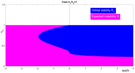
Figure 2. The region of orbital stability ($d^{″}>0$) for $h_1/h_2=1$, $\frac{a\left|a\right|}{b}\in (-4,4)$ and $c^2\in (0,1)$: left half-plane is for $a<0$; right half-plane is for $a>0$.

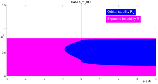
Figure 3. The region of orbital stability ($d^{″}>0$) for $h_1/h_2=0.8$, $\frac{a\left|a\right|}{b}\in (-4,4)$ and $c^2\in (0,0.8)$: left half-plane is for $a<0$; right half-plane is for $a>0$.

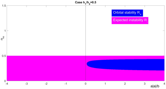
Figure 4. The region of orbital stability ($d^{″}>0$) for $h_1/h_2=0.5$, $\frac{a\left|a\right|}{b}\in (-4,4)$ and $c^2\in (0,0.5)$: left half-plane is for $a<0$; right half-plane is for $a>0$.

Theorem 4.

Suppose $f\left(u\right)=a{u}^2+b{u}^3$, $a\ne 0$, $b>0$, $h_1>0$ and $h_2>0$. Then, the solitary wave ${\overrightarrow{\phi }}_c$ is defined for every $c^2\in I$, $I:=\left(0,min\left(1,\frac{h_1}{h_2}\right)\right)$. Moreover, we have the following behavior of $d^{″}\left(c\right)$ when $c^2$ approaches end points of I:

(a) 

for $c^2\to 0$:

there exists a constant ${\theta }_1\in (0,1)$ such that $d^{″}\left(c\right)<0$ whenever $c^2\in \left(0,{\theta }_1\right)$.

(b) 

for $c^2\to min\left(1,\frac{h_1}{h_2}\right)$, $c^2<min\left(1,\frac{h_1}{h_2}\right)$:

(b₁) 

if $h_1>h_2$, then there exist constants ${\theta }_2\in (0,1)$ and ${\theta }_3\in (0,1)$ such that:

∗

if $a>0$, then $d^{″}\left(c\right)>0$ whenever $c^2\in \left({\theta }_2,1\right)$. The solitary wave ${\overrightarrow{\phi }}_c$ with velocity $c^2\in \left({\theta }_2,1\right)$ is orbitally stable.

∗

if $a<0$ and $h_1\ge 3h_2$, then $d^{″}\left(c\right)<0$ whenever $c^2\in \left({\theta }_2,1\right)$.

∗

if $a<0$, $h_2<h_1<3h_2$ and $\frac{9(h_1-h_2)(3h_2-h_1)}{h_1{h}_2}<\frac{a^2}{b}$, then $d^{″}\left(c\right)<0$ whenever $c^2\in \left({\theta }_2,1\right)$.

∗

if $a<0$, $h_2<h_1<3h_2$ and $\frac{a^2}{b}<\frac{9(h_1-h_2)(3h_2-h_1)}{h_1{h}_2}$, then $d^{″}\left(c\right)>0$ whenever $c^2\in \left({\theta }_3,1\right)$. The solitary wave ${\overrightarrow{\phi }}_c$ with velocity $c^2\in \left({\theta }_3,1\right)$ is orbitally stable.

(b₂) 

if $h_1=h_2$, then

∗

if $a<0$, then there exists a constant ${\theta }_5\in (0,1)$ such that $d^{″}\left(c\right)<0$ whenever $c^2\in \left(1-{\theta }_5,1\right)$;

∗

if $a>0$, then there exists a constant ${\theta }_6\in (0,1)$ such that $d^{″}\left(c\right)>0$ whenever $c^2\in \left(1-{\theta }_6,1\right)$. The solitary wave ${\overrightarrow{\phi }}_c$ with velocity $c^2\in \left(1-{\theta }_6,1\right)$ is orbitally stable.

(b₃) 

if $h_1<h_2$, then there exists a constant ${\theta }_4\in \left(0,\frac{h_1}{h_2}\right)$ such that $d^{″}\left(c\right)<0$ whenever $c^2\in \left(\frac{h_1}{h_2}-{\theta }_4,\frac{h_1}{h_2}\right)$.

Moreover, all constants ${\theta }_i$, $i=1,2,3,4,5,6$ depend on $\frac{a}{\sqrt{b}}$ and $\frac{h_1}{h_2}$.

For completeness, in the following theorem we consider the remaining conditions $a=0$, $b>0$ in (B). In this case, we study a single cubic nonlinearity instead of a combined quadratic-cubic nonlinearity (4).

Theorem 5.

Suppose $f\left(u\right)=b{u}^3$, $b>0$. Then, the solitary wave ${\overrightarrow{\phi }}_c$ is defined for $c^2\in \left(0,min(\frac{h_1}{h_2},1)\right)$. Moreover,

(i) 

if $h_1\ge h_2$, then there exists a constant ${\sigma }_1\in (0,1)$ defined in (A12), such that $d^{″}\left(c\right)<0$ whenever $c^2\in (0,{\sigma }_1)$ and $d^{″}\left(c\right)>0$ whenever $c^2\in ({\sigma }_1,1)$. The solitary wave ${\overrightarrow{\phi }}_c$ is orbitally stable for $c^2\in ({\sigma }_1,1)$. For $h_1=h_2$, we have ${\sigma }_1=\frac{1}{3}$.

(ii) 

if $h_1<h_2$, then there exists a constant $h^{*}\in (0,1)$ defined in (A13), $h^{*}\approx 0.538759214$, such that for $\frac{h_1}{h_2}<h^{*}$ and $c^2\in \left(0,\frac{h_1}{h_2}\right)$ the inequality $d^{″}\left(c\right)<0$ holds.

If $1>\frac{h_1}{h_2}>h^{*}$, then there exist constants ${\sigma }_2$ and ${\sigma }_3$, $0<{\sigma }_2<{\sigma }_3<\frac{h_1}{h_2}$ defined in (A15) such that $d^{″}\left(c\right)<0$ whenever $c^2\in (0,{\sigma }_2)\cup ({\sigma }_3,\frac{h_1}{h_2})$, and $d^{″}\left(c\right)>0$ whenever $c^2\in ({\sigma }_2,{\sigma }_3)$. The solitary wave ${\overrightarrow{\phi }}_c$ with velocity $c^2\in ({\sigma }_2,{\sigma }_3)$ is orbitally stable.

If $\frac{h_1}{h_2}=h^{*}$, then there exists a constant ${\sigma }_4\in \left(0,h^{*}\right)$ defined in (A16), ${\sigma }_4\approx 0.368121369$, such that $d^{″}\left(c\right)<0$ whenever $c^2\in \left(0,{\sigma }_4\right)\cup \left({\sigma }_4,h^{*}\right)$.

Moreover, all constants ${\sigma }_i$, $i=1,2,3,4$ depend on $\frac{h_1}{h_2}$ only.

The proofs of Theorem 4 and Theorem 5 are given in the Appendix A.

Let us discuss some implications of our results for solitary wave orbital stability.

Remark 4.

Let us recall that for $h_1>h_2>0$ and an arbitrary single nonlinearity $f\left(u\right)={\left|u\right|}^{p-1}u$, $p>1$ the orbital stability of solitary waves is analytically and numerically studied in [31]. In Theorem 5$\left(i\right)$, we exhaustively investigate the orbital stability of solitary waves for single cubic nonlinearity ($p=3$), generalizing the result in [31]. We note that the function $d\left(c\right)$ in (A10) coincides with formula (4.1) in [31] for $p=3$ with $d\left(0\right)=\frac{4\sqrt{h_2}}{3b}$, see in [39]. Moreover, in Theorem 5(ii), we prove for the first time the orbital stability of the solitary wave ${\overrightarrow{\phi }}_c$ in the case $h_1<h_2$.

Remark 5.

We establish here only the stability result of solitary waves (see Theorem 2), not the instability result. For a quadratic-cubic nonlinearity, we prove that in some regions function $d\left(c\right)$ is concave, which is a necessary condition for instability. Therefore, we hypothesize that solitary waves are unstable in that region and in the following call these solitary waves “expected unstable” there.

Remark 6.

We study here and in [28] the stability of solitary waves with small values of velocities, i.e., $c^2<1$. The investigation of stability/instability of solitary waves for double dispersion equation with large values of velocities $c^2>1$ remains an open problem.

5. Discussion

In this section, we analyze the dynamics of the stability regions with respect to the changes of the problem parameters.

In Figure 1, Figure 2, Figure 3 and Figure 4, we show the dependence of the sign of $d^{″}$ on the parameters $\frac{h_1}{h_2}$, $\frac{a}{\sqrt{b}}$, and $c^2$, see (A3) and (A4). We fix parameters $h_1$, $h_2$, a, and b and compute the values of $d^{″}\left(c\right)$ by formula (17). In the plane $\{\frac{a\left|a\right|}{b},c^2\}$ with the abscissa $\frac{a\left|a\right|}{b}$ and ordinate $c^2$, we find the regions with different signs of $d^{″}\left(c\right)$. When $\frac{a\left|a\right|}{b}$ is fixed, the vertical line defines the intervals of c, where the solitary wave is stable or possibly unstable. The color blue depicts the region ${\mathcal{R}}_{+}$ of orbital stability of solitary waves where $d^{″}\left(c\right)>0$. The color pink represents the region ${\mathcal{R}}_{-}$, where $d^{″}\left(c\right)<0$ and instability of solitary waves is expected.

Similarly to the investigation in [40], we discuss the influence of the dispersion parameters $h_1$, $h_2$ and the nonlinearity parameters a and b on the stability of solitary waves. In Figure 1, Figure 2, Figure 3 and Figure 4, we demonstrate the regions of stability/expected instability for typical parameters of the problem. According to the assumptions of Theorem 4, further on we suppose that $b>0$.

We observe that for every admissible combination of parameters $\frac{h_1}{h_2}$ and $\frac{a\left|a\right|}{b}$ function $d^{″}\left(c\right)$ is negative in a small neighborhood of $c=0$, i.e., the solitary waves are expected to be unstable for velocities close to $c=0$.

Case $\mathbf{a}>\mathbf{0}$. First, let $a>0$ (see the right half-planes of Figure 1, Figure 2, Figure 3 and Figure 4). Let us consider the case $h_1>h_2$, which is called an “anomalous dispersion case” in [40]. Then, for every fixed value of $\frac{a\left|a\right|}{b}$, the function $d^{″}\left(c\right)$ changes its sign exactly one time in the interval $c^2<1$, see the right half-plane of Figure 1. Let $c^{*}=c^{*}\left(\frac{a\left|a\right|}{b}\right)$ be such that $d^{″}\left(c^{*}\right)=0$. Then, the solitary waves are stable for every $c^2>c^{*}$ and expected to be unstable for every $c^2<c^{*}$. In the “balanced dispersion case” $h_1=h_2$ the situation is the same as in the case $h_1>h_2$, see Figure 2.

In the “normal dispersion case” $h_1<h_2$ (see in [40]) the situation changes (see right half-planes of Figure 3 and Figure 4): for every fixed value of $\frac{a\left|a\right|}{b}$ the function $d^{″}\left(c\right)$ may change its sign two, one, or zero times depending on $c^2$. Close to the end points of the velocity interval ($c=0$ and $c^2=\frac{h_1}{h_2}$) we have $d^{″}\left(c\right)<0$, i.e., in the plane $\{\frac{a\left|a\right|}{b},c^2\}$ the region ${\mathcal{R}}_{-}$ is disconnected for $\frac{h_1}{h_2}>h^{*}$ and becomes connected for $\frac{h_1}{h_2}<h^{*}$. We recall that $h^{*}\approx 0.538759214$ is defined in Theorem 5 (ii).

Let us analyze the dynamics of the regions ${\mathcal{R}}_{+}$ and ${\mathcal{R}}_{-}$ for fixed positive $a>0$, and $\frac{h_1}{h_2}$ changing from values greater than one to values smaller than $h^{*}<1$. In this case, the solitary waves with velocities $c^2$ close to $min\left\{\frac{h_1}{h_2},1\right\}$ are stable for $\frac{h_1}{h_2}>1$ and are possibly unstable for $\frac{h_1}{h_2}<1$. Moreover, when $\frac{h_1}{h_2}<h^{*}$ the region of stability goes away from the line $\frac{a\left|a\right|}{b}=0$.

Case $\mathit{a}<\mathbf{0}$. We assume $\mathit{a}<\mathbf{0}$ (see the left half-planes of Figure 1, Figure 2, Figure 3 and Figure 4). We observe that the regions of orbital stability and expected instability depend on the value of ratio $\frac{\mathit{a}\left|\mathit{a}\right|}{\mathit{b}}$ as in the case $\mathit{a}>\mathbf{0}$. Moreover, when the ratio of nonlinearity parameters $\frac{\mathit{a}\left|\mathit{a}\right|}{\mathit{b}}$ is sufficiently small, all waves with high velocities are possibly unstable.

We analyze the dynamics of ${\mathcal{R}}_{+}$ for $\mathit{a}<\mathbf{0}$ and $\frac{{\mathit{h}}_{\mathbf{1}}}{{\mathit{h}}_{\mathbf{2}}}$ in the intervals $(\mathbf{1},\mathbf{3})$ (see Figure 1 for $\frac{{\mathit{h}}_{\mathbf{1}}}{{\mathit{h}}_{\mathbf{2}}}=\mathbf{1}.\mathbf{3}$), $({\mathit{h}}^{*},\mathbf{1})$ (see Figure 3 for $\frac{{\mathit{h}}_{\mathbf{1}}}{{\mathit{h}}_{\mathbf{2}}}=\mathbf{0}.\mathbf{8}$) and $(\mathbf{0},{\mathit{h}}^{*})$ (see Figure 4 for $\frac{{\mathit{h}}_{\mathbf{1}}}{{\mathit{h}}_{\mathbf{2}}}=\mathbf{0}.\mathbf{5}$, respectively). We observe that the region of stability ${\mathcal{R}}_{+}$ shrinks and disappears for $\frac{{\mathit{h}}_{\mathbf{1}}}{{\mathit{h}}_{\mathbf{2}}}<{\mathit{h}}^{*}$. For parameters $\frac{{\mathit{h}}_{\mathbf{1}}}{{\mathit{h}}_{\mathbf{2}}}<{\mathit{h}}^{*}$, all solitary waves are expected to be unstable.

In conclusion, the behavior of stability/expected instability regions is quite complicated; it depends on the values of $\frac{{\mathit{h}}_{\mathbf{1}}}{{\mathit{h}}_{\mathbf{2}}}$ and $\frac{\mathit{a}\left|\mathit{a}\right|}{\mathit{b}}$ (equivalently on $\frac{\mathit{a}}{\sqrt{\mathit{b}}}$). That is why in Theorem 4, we prove orbital stability at the end points of the existence interval of the velocity of solitary waves.

In the case $\mathit{a}=\mathbf{0}$, i.e., $\frac{{\mathit{a}}^{\mathbf{2}}}{\mathit{b}}=\mathbf{0}$, the plots on Figure 1, Figure 2, Figure 3 and Figure 4 confirm the results in Theorem 5(i) and Theorem 5(ii). For example, when $\frac{{\mathit{h}}_{\mathbf{1}}}{{\mathit{h}}_{\mathbf{2}}}=\mathbf{0}.\mathbf{8}>{\mathit{h}}^{*}\approx \mathbf{0}.\mathbf{538759214}$, the interval of orbital stability ${\mathit{\sigma }}_{\mathbf{2}}<{\mathit{c}}^{\mathbf{2}}<{\mathit{\sigma }}_{\mathbf{3}}$ is illustrated on the vertical axis $\mathit{a}=\mathbf{0}$ of Figure 3.

6. Conclusions

In this paper we investigate the orbital stability of solitary waves to system (9) with velocities ${\mathit{c}}^{\mathbf{2}}<\mathbf{1}$, as well as the stability of solitary waves to problem (1) –(3). The proof of the orbital stability is based on the convexity of function $\mathit{d}\left(\mathit{c}\right)$ connected to some conserved quantities of the problem.

We derive an explicit expression of ${\mathit{d}}^{″}\left(\mathit{c}\right)$ for quadratic-cubic nonlinearity (4) and parameters $\mathit{b}>\mathbf{0}$, $\mathit{a}\in \mathbb{R}$, ${\mathit{c}}^{\mathbf{2}}\in \left[\mathbf{0},\mathbf{min}\left(\mathbf{1},\frac{{\mathit{h}}_{\mathbf{1}}}{{\mathit{h}}_{\mathbf{2}}}\right)\right)$. In Theorem 4, we analyze the sign of ${\mathit{d}}^{″}\left(\mathit{c}\right)$ for values of $\mathit{c}$ sufficiently close to end points 0 and $\mathbf{min}\left(\mathbf{1},\frac{{\mathit{h}}_{\mathbf{1}}}{{\mathit{h}}_{\mathbf{2}}}\right)$ of the existence interval for $\mathit{c}$ and $\mathit{a}\ne \mathbf{0}$. Additionally, in Theorem 5, we study exhaustively the sign of ${\mathit{d}}^{″}\left(\mathit{c}\right)$ and orbital stability of solitary waves in the particular case of cubic nonlinearity, i.e., $\mathit{a}=\mathbf{0}$, $\mathit{b}>\mathbf{0}$ in (4).

The results in Theorem 5(i) in the present paper generalize those in [31] for the double dispersion equation with a single cubic nonlinearity. In Theorem 5(ii), we prove for the first time orbital stability of solitary waves ${\overrightarrow{\mathit{\phi }}}_{\mathit{c}}$ in the case ${\mathit{h}}_{\mathbf{1}}<{\mathit{h}}_{\mathbf{2}}$.

Our investigation shows that the orbital stability of solitary waves depends on the parameters $\mathit{a}$, $\mathit{b}$, ${\mathit{h}}_{\mathbf{1}}$, and ${\mathit{h}}_{\mathbf{2}}$ of the problem through the quantities $\frac{\mathit{a}}{\sqrt{\mathit{b}}}$ and $\frac{{\mathit{h}}_{\mathbf{1}}}{{\mathit{h}}_{\mathbf{2}}}$. The orbital stability of solitary waves ${\overrightarrow{\mathit{\phi }}}_{\mathbf{c}}$ is sensitive to the changes of the values of $\frac{\mathit{a}}{\sqrt{\mathit{b}}}$ and $\frac{{\mathit{h}}_{\mathbf{1}}}{{\mathit{h}}_{\mathbf{2}}}$. More precisely, for fixed parameters $\frac{\mathit{a}}{\sqrt{\mathit{b}}}$ and $\frac{{\mathit{h}}_{\mathbf{1}}}{{\mathit{h}}_{\mathbf{2}}}$, the function ${\mathit{d}}^{″}\left(\mathit{c}\right)$ may change its sign zero, one, or two times in the interval ${\mathit{c}}^{\mathbf{2}}\in \left(\mathbf{0},\mathbf{min}\left(\mathbf{1},\frac{{\mathit{h}}_{\mathbf{1}}}{{\mathit{h}}_{\mathbf{2}}}\right)\right)$.

References

- Porubov, A. Amplification of Nonlinear Strain Waves in Solids; World Scientific: Singapore, 2003. [Google Scholar]
- Porubov, A.; Maugin, G. Longitudinal strain solitary waves in the presence of cubic nonlinearity. Int. J. Nonlinear Mech. 2005, 40, 1041–1048. [Google Scholar] [CrossRef]
- Zhang, S.; Liu, Z. Three kinds of nonlinear dispersive waves in elastic rods with finite deformation. Appl. Math. Mech. Engl. Ed. 2008, 29, 909–917. [Google Scholar] [CrossRef]
- Maugin, G. Nonlinear Waves in Elastic Crystals; Oxford University Press: Oxford, UK, 1999; pp. 1–314. [Google Scholar]
- Falk, F.; Laedke, E.; Spatschek, K. Stability of solitary-wave pulses in shape-memory alloys. Phys. Rev. B 1987, 36, 3031–3041. [Google Scholar] [CrossRef] [PubMed]
- Christov, C.I. An energy-consistent dispersive shallow-water model. Wave Motion 2001, 34, 161–174. [Google Scholar] [CrossRef]
- Xu, R.; Liu, Y. Global existence and nonexistence of solution for Cauchy problem of multidimensional double dispersion equations. J. Math. Anal. Appl. 2009, 359, 739–751. [Google Scholar] [CrossRef]
- Kutev, N.; Kolkovska, N.; Dimova, M. Global existence to generalized Boussinesq equation with combined power-type nonlinearities. J. Math. Anal. Appl. 2014, 410, 427–444. [Google Scholar] [CrossRef]
- Heimburg, T.; Jackson, A.D. On soliton propagation in biomembranes and nerves. Proc. Natl. Acad. Sci. USA 2005, 102, 9790–9795. [Google Scholar] [CrossRef] [PubMed]
- Heimburg, T.; Jackson, A.D. On the action potential as a propagating density pulse and the role of anaesthetics. Biophys. Rev. Lett. 2007, 57, 57–78. [Google Scholar] [CrossRef]
- Cimpoiasu, R. Nerve pulse propagation in biological membranes: Solitons and other invariant solutions. Int. J. Biomath. 2016, 9, 1650075. [Google Scholar] [CrossRef]
- Engelbrecht, J.; Tamm, K.; Peets, T. On mathematical modeling of solitary pulses in cylindrical biomembranes. Biomech. Model. Mechanobiol. 2015, 14, 159–167. [Google Scholar] [CrossRef]
- Peets, T.; Tamm, K.; Engelbrecht, J. On the role of nonlinearities in the Boussinesq-type wave equations. Wave Motion 2017, 71, 113–119. [Google Scholar] [CrossRef]
- Peets, T.; Tamm, K. Mathematics of nerve signals. In Applied Wave Mathematics II; Berezovski, A., Soomere, T., Eds.; Springer: Cham, Switzerland, 2019; Volume 6, pp. 207–238. [Google Scholar]
- Erbay, H.A.; Erbay, S.; Erkip, A. Existence and stability of traveling waves for a class of nonlocal nonlinear equations. J. Math. Anal. Appl. 2015, 425, 307–336. [Google Scholar] [CrossRef]
- Höwing, J. Stability of large- and small-amplitude solitary waves in the generalized Korteweg—De Vries and Euler—Korteweg-Boussinesq equations. J. Differ. Equ. 2011, 251, 2515–2533. [Google Scholar] [CrossRef]
- Lin, Z. Instability of nonlinear dispersive solitary waves. J. Funct. Anal. 2008, 255, 1191–1224. [Google Scholar] [CrossRef]
- Quintero, J.R. Nonlinear Stability of a One-Dimensional Boussinesq Equation. J. Dyn. Differ. Equ. 2003, 15, 125–142. [Google Scholar] [CrossRef]
- Smereka, P. A remark on the solitary wave stability for a Boussinesq equation. In Nonlinear Dispersive Wave Systems; World Scientific: Singapore, 1992; pp. 255–263. [Google Scholar]
- Stube, J. Existence and stability of solitary waves of Boussinesq type equations. Port. Mat. 1989, 46, 501–516. [Google Scholar]
- Grillakis, M.; Shatah, J.; Strauss, W.A. Stability theory of solitary waves in the presence of symmetry. J. Funct. Anal. 1987, 74, 160–197. [Google Scholar] [CrossRef]
- Bona, J.L.; Souganidis, P.E.; Strauss, W.A. Stability and Instability of Solitary Waves of Korteweg-de Vries Type. Proc. R. Soc. Lond. Ser. A Math. Phys. Sci. 1987, 411, 395–412. [Google Scholar]
- Bona, J.L.; Sachs, R. Global existence of smooth solutions and stability of solitary waves for a generalized Boussinesq equation. Commun. Math. Phys. 1988, 118, 15–19. [Google Scholar] [CrossRef]
- Liu, Y. Instability of solitary waves for generalized Boussinesq equation. J. Dyn. Differ. Equ. 1993, 5, 537–558. [Google Scholar] [CrossRef]
- Li, B.; Ohta, M.; Wu, Y.; Xue, J. Instability of the solitary waves for the generalized Boussinesq equations. SIAM J. Math. Anal. 2020, 52, 3192–3221. [Google Scholar] [CrossRef]
- Liu, Y. Instability and blow-up of the solutions to a generalized Boussinesq equation. SIAM J Math. Anal. 1995, 26, 1527–1546. [Google Scholar] [CrossRef]
- Liu, Y.; Ohta, M.; Todorova, G. Strong instability of solitary waves for nonlinear Klein-Gordon equations and generalized Boussinesq equations. In Annales de l’Inst. Henri Poincare (c) Non-Linear Analysis; Elsevier: Amsterdam, The Netherlands, 2007; Volume 24, pp. 539–549. [Google Scholar]
- Kolkovska, N.; Dimova, M.; Kutev, N. Stability or instability of solitary waves to double dispersion equation with quadratic-cubic nonlinearity. Math. Comput. Simul. 2017, 133, 249–264. [Google Scholar] [CrossRef]
- Dimova, M.; Kolkovska, N.; Kutev, N. Orbital stability or instability of solitary waves to generalized Boussinesq equation with quadratic-cubic nonlinearity. C. R. Acad. Bulg. Des Sci. 2018, 71, 1011–1018. [Google Scholar]
- Zhang, W.; Li, X.; Li, S.; Chen, X. Orbital stability of solitary waves for generalized Boussinesq equation with two nonlinear terms, Commun. Nonlinear Sci. Numer. Simulat. 2018, 59, 629–650. [Google Scholar] [CrossRef]
- Erbay, H.A.; Erbay, S.; Erkip, A. Instability and stability properties of traveling waves for the double dispersion equation. Nonlinear Anal. 2016, 133, 1–14. [Google Scholar] [CrossRef][Green Version]
- Wang, Y.; Mu, C.; Deng, J. Strong instability of solitary-wave solutions for a nonlinear Boussinesq equation. Nonlinear Anal. 2008, 69, 1599–1614. [Google Scholar] [CrossRef]
- Christov, C.I. Conservative difference scheme for Boussinesq model of surface water. In Proceedings ICFD 5; Oxford University Press: London, UK, 1996; pp. 343–349. [Google Scholar]
- Kolkovska, N.; Dimova, M. A new conservative finite difference scheme for Boussinesq paradigm equation. Cent. Eur. J. Math. 2012, 10, 1159–1171. [Google Scholar] [CrossRef]
- Kolkovska, N.; Vucheva, V. Invariant preserving schemes for double dispersion equations. Adv. Differ. Equ. 2019, 2019, 216. [Google Scholar] [CrossRef]
- Pava, J.A. Nonlinear Dispersive Equations: Existence and Stability of Solitary and Periodic Travelling Wave Solutions; American Mathematical Society: Providence, RI, USA, 2009. [Google Scholar]
- Natali, F.; Pastor, A.; Cristófani, F. Orbital stability of periodic traveling-wave solutions for the log-KdV equation. J. Differ. Equ. 2017, 263, 2630–2660. [Google Scholar] [CrossRef]
- Levandosky, S. Stability and instability of fourth-order solitary waves. J. Dyn. Differ. Equ. 1998, 10, 151–188. [Google Scholar] [CrossRef]
- Kutev, N.; Kolkovska, N.; Dimova, M. Theoretical and numerical aspects for global existence and blow up for the solutions to Boussinesq paradigm equation. In AIP Conference Proceedings; American Institute of Physics: College Park, MD, USA, 2011; Volume 1404, pp. 68–76. [Google Scholar]
- Engelbrecht, J.; Tamm, K.; Peets, T. On solutions of a Boussinesq-type equation with amplitude-dependent nonlinearities: The case of biomembranes. Philos. Mag. 2017, 97, 967–987. [Google Scholar] [CrossRef]
- Kurosh, A.G. Higher Algebra; Mir Publishers: Moscow, Russia, 1972. [Google Scholar]
Publisher’s Note: MDPI stays neutral with regard to jurisdictional claims in published maps and institutional affiliations. |
© 2021 by the authors. Licensee MDPI, Basel, Switzerland. This article is an open access article distributed under the terms and conditions of the Creative Commons Attribution (CC BY) license (https://creativecommons.org/licenses/by/4.0/).